
Do Risky Scenarios Affect Forecasts of Savings and Expenses?


1
Department of Business Informatics and Operations Management, Faculty of Economics and Business Administration, Ghent University, 9000 Ghent, Belgium
2
Department of Marketing, Operations and Systems, Newcastle Business School, Northumbria University, Newcastle upon Tyne NE1 8ST, UK
3
Management School, University of Stirling, Stirling FK9 4LA, UK
*
Author to whom correspondence should be addressed.
Forecasting 2022, 4(1), 307-334; https://0-doi-org.brum.beds.ac.uk/10.3390/forecast4010017
Submission received: 14 December 2021
/
Revised: 8 February 2022
/
Accepted: 18 February 2022
/
Published: 21 February 2022
(This article belongs to the Section Forecasting in Economics and Management)
Abstract
:Many people do not possess the necessary savings to deal with unexpected financial events. People’s biases play a significant role in their ability to forecast future financial shocks: they are typically overoptimistic, present-oriented, and generally underestimate future expenses. The purpose of this study is to investigate how varying risk information influences people’s financial awareness, in order to reduce the chance of a financial downfall. Specifically, we contribute to the literature by exploring the concept of ‘nudging’ and its value for behavioural changes in personal financial management. While of great practical importance, the role of nudging in behavioural financial forecasting research is scarce. Additionally, the study steers away from the standard default choice architecture nudge, and adds originality by focusing on eliciting implementation intentions and precommitment strategies as types of nudges. Our experimental scenarios examined how people change their financial projections in response to nudges in the form of new information on relevant risks. Participants were asked to forecast future expenses and future savings. They then received information on potential events identified as high-risk, low-risk or no-risk. We investigated whether they adjusted their predictions in response to various risk scenarios or not and how such potential adjustments were affected by the information given. Our findings suggest that the provision of risk information alters financial forecasting behaviour. Notably, we found an adjustment effect even in the no-risk category, suggesting that governments and institutions concerned with financial behaviour can increase financial awareness merely by increasing salience about possible financial risks. Another practical implication relates to splitting savings into different categories, and by using different wordings: A financial advisory institution can help people in their financial behaviour by focusing on ‘targets’, and by encouraging (nudging) people to make breakdown forecasts rather than general ones.
1. Introduction
Many households do not have the necessary savings to deal with unexpected shocks, such as a car breaking down or a family member becoming unemployed [1,2,3]. Consequently, many people suffer economic insecurity and are at risk for future economic problems [4]. The issue is further complicated by people’s behavioural tendencies: they are more oriented towards the present than towards the future [5,6], prefer instant gratification over long-term benefits [7,8,9], underestimate a future rise in expenses compared to a rise in income, and underestimate the risk of unexpected expenses in the near future compared to those they experienced in the near past [10]. Additionally, the broader literature on judgment and decision-making teaches us that people suffer from a general optimism bias [11] and tend to ignore pessimistic scenarios and focus instead on the positive ones [12]. Consequently, these factors all add up to an underestimation of future expenses, increasing the risk of households without savings to fall into economic turmoil. Behavioural decision research has focused mostly on identifying biases and proving that people are not always capable of making decisions that are in their own self-interest [13]. Ratner et al. [14] suggest that behavioural decision research should focus on helping people make decisions, and not just on defining what goes awry. One way to do this is by means of ‘nudging’ people’s behaviour in the right direction [13]. Nudges can lead to altered behaviour by structuring the choice task differently or in the description of the choice options [15]. Therefore, the objective of this study is to test, with the use of scenarios, how to best aid people’s judgment in predicting financial risks and how to nudge them towards an improved financial wellbeing.
The main research question of this project focuses on the effect of risk information on participant’s forecasts of savings and expenses. We will investigate this in a scenario-based behavioural experiment (N = 325), specifically, whether: (1) participants adjust their forecasts based on the information they receive, (2) whether this adjustment is different for savings and expenses and savings, and (3) what the effect of different types of risks is (low-risk, high-risk, control/no-risk).
2. Literature
In this study we look at two aspects of financial decision making: forecasting expenses and forecasting savings. Savings are a major concern for many households. Savings rates are historically low and are combined with high debt burdens [16]. This combination puts households at an economic risk. When looking at emergency savings, the general rule of thumb is to have at least three months’ worth of a household’s typical monthly expense. These savings are necessary to protect the household against economic risks such as unemployment, household appliances breaking down or unanticipated medical costs. However, surveys have shown that about half of respondents were not able to come up with $2000 within a month’s time for emergencies [3], which can lead to problematic debt. The picture is not much better when looking at retirement savings. In the USA, it has been reported that around half of the population does not have sufficient savings for retirement [17,18]. In the UK, one third of people have no additional retirement savings on top of their government pension [19]. In many countries, people can join pension schemes at work or via a national retirement scheme [20]. However, not everyone joins a retirement scheme, and some of those who do become more complacent about their retirement [21]. People need to be nudged in the right direction [20]. This can even be done subliminally [22]. Regarding expenses, people are quite capable of forecasting and monitoring their regular expenses. However, exceptional expenses are consistently underestimated, and are more frequent than is generally assumed to be the case. This is probably due to a too narrow definition of what constitutes ‘exceptional’ [23]. All the above issues can be framed within a behavioural economic framework. Several biases play an important role in our savings and expenses fallacies.
First, there are anomalies in the intertemporal choices we make, compared to what a rational model would predict. An intertemporal choice refers to the decisions we make when we choose between something smaller sooner or something larger later. For instance, humans tend to make plans for the future which they do not act upon when the time is near. We might make a decision to save for a future major purchase but indulge in luxury spending today. This is termed the common difference effect [24] and has been replicated both in the laboratory and in the field for a wide range of topics. For money, results are mixed. Some find evidence for the common difference effect, others find a lack of it or even a reverse effect [25]. Whenever it does occur, the effect is related to present bias. We attach more value to something at present than to something in the future [25] This effect is also termed hyperbolic discounting. Thaler [26] for instance, found a clear preference for a small amount of money received today over a larger amount received later. The longer the time delay of the ‘later’-choice, the stronger the preference for the smaller amount. Furthermore, people have been found to give more weight to immediate spending as compared to later saving. The weight closer to the decision period is larger, resulting in hyperbolic functions, hence the term hyperbolic discounting. Given that people are more oriented towards the present than the future [5,6], the general advice often given to people wanting to save more is to be less myopic and to be more proactive in preparing financially for the future.
A second deviation from rational decision making is the levels of overoptimism that are found when forecasting financial matters. For instance, we underestimate the future rise in expenses compared to a rise in income and underestimate the risk of unexpected expenses in the near future compared to those they experienced in the near past [10]. Overoptimism is found in a wide range of domains [11] but seems to be particularly persistent in financial decision making and independent of optimism as a personality trait [27]. When asked to think about the future, people generate a limited number of scenarios in their head. These usually incorporate their hopes and preferences, leading to a generally overoptimistic scenario [28].
Hyperbolic discounting or present bias combines with financial overoptimism in Resource Slack Theory. Resource slack is “... the perceived surplus of a given resource available to complete a focal task without causing failure to achieve goals associated with competing uses of the same resource.” [27] (p. 23). This resource slack is perceived as being greater in the future than in the near present. In other words, people are overoptimistic about the resources they will have available in a distant time frame, but less so in the time frame near to the decision-making period.
One possible explanation for this can be found in construal level theory [29]. This theory states that things become less abstract when they get closer in time to the decision making period. As such, a mental representation of something in the future can be changed by drawing attention to it and by making it more salient. An initial nudge to make savings and expenses in the future more salient consists of making people think about concrete savings goals [30]. In this study, we focus on risk information as a way of making savings and expenses more realistic and less overoptimistic. We examine the potential effects of using target setting, categorical breakdowns, and risk scenarios as tools towards making more realistic (and less overoptimistic) savings and expenses forecasts. These scenarios and the information they contain can be seen as ‘nudges’—factors that alter human behaviour [31]. Löfgren and Nordblom [32] framed this within a theoretical framework based on attentive and inattentive decisions, in line with the work by Gigerenzer and Gaissmaier [33]. They posit that rational choices, which are well-informed and utility-maximized, require significant cognitive effort. To avoid this effort, people turn towards heuristics, which may lead to mistakes. While heuristics can be useful in lightening our cognitive load, they may also lead to biases [34]. These include the biases mentioned above: the common difference effect, overoptimism, and hyperbolic discounting or present bias. A nudge can serve as a ‘boost’ that reduces cognitive effort and thus makes an attentive choice more likely, and a reliance on heuristics and consequent biases less likely [32].
Nudging research was originally stated to be for the betterment of “health, wealth and happiness” [31]. Yet, a meta-analysis by Hummel and Maedche [35] found that most nudging research centres specifically around health, such as with dietary choices (for a meta-analysis, see [36]), for instance. Nudges for ‘wealth’ have similarly been investigated before, though to a lesser extent: only 12 out of 100 studies investigated in the meta-analysis (as opposed to 38 involving health, followed in second place by 19 studies on energy; [35]). Thaler and Benartzi’s [30] Save More Tomorrow (SMART) program is an early adopter of nudges in the form of influencing financial choice architecture: they proposed an opt-out, rather than opt-in approach for employee’s retirement savings, significantly increasing retirement savings. This US-based study has been replicated in a variety of countries, such as Denmark [37] and Spain [38]. This type of study is an example of nudging via ‘default choice architecture’. Hummel and Maedche [35] note that where financial nudges were concerned, most of the investigated effect sizes in their meta-analyses were in this category. This was followed closely by the provision of reminders as a nudging tool. Between the publication of the meta-analysis and the current study, other financial nudging studies have been few and far between, with most research focusing on health-related behaviours surrounding the pandemic (e.g., social distancing [39]; vaccination [40]; hand hygiene [41]). Empirical nudging studies on financial behaviour since the 2019 meta-analysis are scarce, although some do exist (e.g., choice architecture in retirement plans [42]; reminders for credit card payments [43]; information provision for credit card payments [44]). However, to the best of the authors’ knowledge, no recent nudging studies on financial behaviour with regard to savings or risk exist. Additionally, we chose a new approach in that we focus on eliciting implementation intentions and precommitment strategies [45] rather than the more common default choice of architecture nudge.
Our research questions focus on whether participants adjust their forecasts based on the information they receive when asked about their financial intentions of savings and expenses, whether any such adjustment is different for savings than for expenses, and what the potential effects of different risk levels are on forecasts.
Extant work on judgmental forecast adjustments emphasizes the important role that scenarios play in encouraging individuals to consider alternative outcomes, thus strengthening the forecast message [46]. Three factors are of importance here [47] (Goodwin, Gönül, & Önkal, 2019): (1) The biases described above with regard to personal financial forecasting; (2) Scenario effectiveness; and (3) Framing effects. First, as elaborated in the beginning of this literature section, certain biases are associated with judgmental forecasting of personal finances. An important goal of the judgmental forecasting field has always been the documentation and mitigation of these biases. The use of decision support systems as a means of mitigation is investigated (e.g., [48]). In organisations, for instance, it is commonplace to use a forecasting system to help make more accurate predictions based on hard data rather than on personal intuition. However, a typical household does not rely on software to make forecasts. As a consequence, mitigation for judgmental biases needs to be looked for somewhere else. Here we turn to the provision of information as a decision support system. One way to achieve this is to work with hypothetical scenarios which make certain financially relevant information more salient and promote future-oriented thinking (see construal level theory and nudging theory above). This brings us to the second factor of importance: the effectiveness of using scenarios. It has long been argued that the use of scenarios can mitigate problems associated with cognitive biases [46,49]. People are drawn to scenarios, more so than to ‘dry’ numbers, because we are drawn to narratives (e.g., [50]). In a study on scenarios as forecasting advice, participants rated the scenarios as ‘useful’ and ‘informative’ [46]. The content of the scenarios matter. Furthermore, the framing, which is the third factor of importance in our study, is varied within and between studies, thereby resulting in differential effects. A typical example of scenario framing in forecasting studies is the provision of a best-case (optimistic) and worst-case (pessimistic) scenario, and to vary the strength of the message (e.g., [46,51]). As discussed in the bias section, we find overoptimism and lack of future orientation everywhere when it comes to forecasting personal finances. We therefore focus on a negative frame so as to make people more aware [52] of potential financial risks, and thus, to encourage them to revise overoptimistic, present-oriented forecasts. Potential financial risks are events that disrupt the household’s financial balance [53]. In its simplest form, financial balance can be at risk due to a decrease in income, or an increase in expenses. The amount of disposable income is an important component in household financial fragility [54]. Previous research has shown that this income is a vital player in saving rates, which increases substantially with increased income [55]. For our first hypothesis, we focus on the income frame and aim to increase the salience of unexpected downfalls. If a positive correlation exists between income and savings [55], we can hypothesize that a negatively framed situation about income will have a negative impact on forecasted savings:
Hypothesis 1 (H1).
Savings forecasts will be adjusted downward for individuals receiving an unexpected income-loss scenario.
On the other side of the household financial balance is how much expenses a household has. Expected future expenses will likely be based on those experienced in the recent past, as these are more salient. It can be expected that by increasing the salience of the expense via a scenario [52], this will encourage people to think more broadly about potential expenses and adjust their expense forecasts upwards based on the new information.
Hypothesis 2 (H2).
Expenses forecasts will be adjusted upward for individuals receiving the unexpected-expense scenario.
These scenarios—income loss and expense increase—can vary in the likelihood of their occurrence and in their severity. Previous studies have found that forecasting adjustments after scenario provision are influenced by the tone of the scenario [56]. It can similarly be hypothesized that financial risk scenarios with varying degrees of risk likelihood imply a certain tone of severity, which, similar to the results of [56], would be positively correlated with the size of the adjustments made. Concretely, we focus on three levels of risk: zero, low, and high. The study cited above [56] found this adjustment size effect to be true regardless of the direction of the adjustment, so we do not hypothesize a distinction between the income-loss and the expense-increase scenario:
Hypothesis 3 (H3).
Individuals receiving high-risk scenarios will make larger forecast adjustments than those receiving low-risk scenarios.
Hypothesis 4 (H4).
Individuals receiving low-risk scenarios will make larger forecast adjustments than those receiving no-risk scenarios.
The previous hypotheses presume the presence of adjustments. However, it is important to note that apparently not everyone will change their estimates, and those that do might not make enough of an adjustment. The latter is due to an anchor-and-adjust heuristic [34], in which people latch on to an original value and do not adjust far enough away from this anchor. The former, not changing estimates, is likely to occur when we look at the advice literature (advice discounting) and, by extension, status quo bias or omission (the decision not to change the status quo; [57]). People are generally not keen on changing their ideas when presented with new information [58]. We expect this will be especially true for participants presented with no-risk scenarios compared to those receiving low-risk and high-risk scenarios. Accordingly, we hypothesize:
Hypothesis 5 (H5).
The proportion of individuals in the no-risk condition that do not adjust their forecasts will be higher than those in the low-risk and high-risk conditions.
The previous theorizing and hypothesis formulation has focused on the diagnosis of adjustment behaviour in savings and expenses. However, these categories are broad strokes. Savings, in particular, has been the subject of research towards varying saving motives (going back to [59]) and how it affects behaviour. This concept of separating financial categories refers to the phenomenon of mental accounting [60]. Antonides, de Groot and van Raaij [61] link mental accounting to having different savings goals, which results in assigning different labels to different savings goals. This ‘mental budgeting’ subsequently leads to better financial management [61]. Simple interventions such as having reminders of savings goals or having separate envelopes for different savings goals can increase the rate of savings [62,63]. Zhan and Sussman [64] note that some financial institutions currently allow for multiple savings accounts with a different label and savings goal for each. In line with these studies on savings behaviour, we can reason that savings forecasts may be equally influenced by the mental accounting effect. The list of savings categories is extensive and differs per country (for an overview, see [65]). Looking at the extant literature, pension savings are the dominating research category. Another savings goal often noted is that of a rainy-day fund or emergency fund—a precautionary savings motive [65]. As we cannot cover all existing categories, we have opted for these two dominating categories (retirement and emergency) and have grouped all other potential goals under ‘personal’ savings. Based on previous literature on savings behaviour and mental accounting, we hypothesize that for savings forecasts, categories matter, such that:
Hypothesis 6 (H6).
The sum of the three savings category forecasts will be more than the general category of predicted savings.
Additionally, as discussed above, financial forecasts suffer from overoptimism [27]. How the intended savings elicitation question is formulated may play a role in the prevalence of this bias [66]. Therefore, in this study, we make a distinction between target savings, expressing a ‘wish’ or a ‘want’, and expected savings, where we add the word ‘realistically’ as a possible way of minimizing the overoptimism effect. We hypothesize that the target savings question will elicit higher estimates than the expected, ‘realistic’ savings question:
Hypothesis 7 (H7).
The estimates for the target savings category will be higher than those of the expected savings category.
We test these hypotheses via behavioural experiments, as detailed next.
3. Materials and Methods
3.1. Pilot Study
To ensure the external validity of the scenarios designed for the main study, and the relevance of the contexts in which these scenarios take place, a pilot test survey was run beforehand. In this preliminary study, 28 participants were asked about potential realistic events that could significantly influence their savings and expenses plans. Based on their textual input, the scenarios for the main experiment were designed. The first question was open-ended: “During our everyday life, we make financial projections on how much we expect to save (savings) or spend (expenses) in the near future. What is something that could happen to you that would influence your financial decision making (i.e., your planned expenses and savings) for the coming months?” Second, participants were asked what the likelihood is of this event occurring (in %) and what the impact would be (scale of 1–5) on their savings and expenses. As shown in Table 1, unexpected expenses and income loss were the two dominant answers and we used these two scenario contexts in our online experiments, adapting scenario context as a between-subjects variable. These scenarios were written with the vision of the founders of scenario research in mind: scenarios are narratives that are vivid, paint the future in detail, and show what may unfold [67]. They depict different possibilities that are plausible, consistent, relevant, transparent, and novel [68]. The pilot study ensured that we used scenarios that were deemed plausible, consistent, and relevant. The writeup focused on transparency by simplifying each thought step as much as possible, and with bringing new information to the foreground (novelty). Attention was paid to making the scenarios relatable by providing psychological cues.
3.2. Participants for the Main Study
The data collection for the main study took place online, via the UK platform Prolific Academic. Participants were assigned randomly to one of three risk conditions (no risk, low risk, high risk) and one of two scenario contexts (expenses/income loss). To obtain sufficient statistical power and ensure a sufficient level of generalizability, an online sample was used with a random sampling method among an international population. To determine sample size, we took into account the experimental design resulting in six groups (two scenario contexts × three risk levels) and the generally accepted indication of a minimum sample size of 30 according to the central limit theorem (CLT, for expected normal distributions [69]). As this is a minimum, and crowdsourcing data needs stringent cleaning, we liberally multiplied the experimental conditions (6) with the CLT minimum (30), with a factor of two, resulting in 360 invited and completed responses. Data cleaning was performed by eliminating those suspected of a lack of attention: those who never adjusted their initial estimates after receiving the risk information while simultaneously giving only incorrect answers to the financial literacy questions, or providing nonsensical answers (e.g., forecasts in the form of ‘12345′). While 360 participants were recruited initially; all analyses are based on 325 participants after this data cleaning. This sample size is considered sufficient to estimate the parameters of a population [69]. External validity was maximized via the pilot study described above, where the information received from the subjects in the pilot study indicated which possible scenarios were uppermost in people’s minds when asked about financial risk factors. Internal validity was maximized by using established standardized measures for the self-rated survey section, as further described under Section 3.4: Variables and Measures.
3.3. Procedure
Participants were invited through the Prolific Academic platform to participate in an online study. They were informed that they would be asked to set savings targets and estimate savings and expenses. If participants chose to participate, they followed the link to the external experimental website (see Figure A1 in Appendix A for screenshots). First, participants were introduced to the topic of the experiment, informed they could stop at any time if they wanted to, and that their data was handled anonymously and according to the Data Protection Act. They were given the contact details of the principal investigator. On the second page, the consent form was presented. By pressing ‘next’, they agreed to participate in the study. On the third page, the actual experiment started: participants were asked to provide target savings as well as forecasts for savings and expenses over the course of the following three months (i.e., for each of three different time horizons) by giving numerical inputs in the text boxes. On the next page, they were asked to give forecasts for distinct subcategories of savings: emergency fund savings, retirement savings, and personal savings. The experimental manipulation took place next, where the participants were provided with scenarios and risk information. Risk was manipulated between-subjects in three categories: high risk, low risk and no risk. Given the findings of the pilot study and the cited literature, we worked with two scenario contexts—one context focusing on unexpected expenses and the other on losing income (with half of the participants receiving a scenario related to an unexpected expense and the remaining half receiving a scenario related to an unexpected loss of income).
Unexpected-expense scenario:
Imagine the following scenario: you come home after a busy day feeling very tired and you are looking forward to a relaxing evening. However, upon arrival, you open your door and the hallway is full of water. A water pipe has broken and water has leaked everywhere. You hurry to shut off the water supply and search the phone number of a local plumber as fast as you can. You call the plumber. After an hour’s wait, he comes by and assesses the damage. The quote he gives amounts to 80% of your monthly income. How does this affect your savings and expenses expense and savings forecasts for the next three months?
The scenario presented above is the high-risk scenario: “The quote he gives amounts to 80% of your monthly income”. In the low-risk scenario, this is replaced by 20% of monthly income. In the no-risk scenario, the participant is informed that “The quote he gives is completely covered by your insurance”.
Unexpected income-loss scenario:
Imagine that you arrive at work on Monday morning. You notice the atmosphere is a bit tense. When you go to check your mailbox, you notice that a company-wide meeting invite has been sent for a meeting later that day. Rumours are flying around that the company is in trouble. You and others are starting to feel quite nervous. When the meeting starts, the rumours are confirmed: the firm is losing money and will need to take action. Unfortunately, this means that some people will have to be let go. The manager informs the audience that, 4 out of 5 people (80%) in your department will hear the bad news by the end of the week.
The scenario presented above presents the high-risk scenario: “4 out of 5 people (80%) in your department will hear the bad news by the end of the week”. In the low-risk scenario, this number is replaced by “1 out of 5 people (20%)”. In the no-risk scenario, the participant is informed that “The manager informs the audience that, fortunately, no one in your department is going to be fired”.
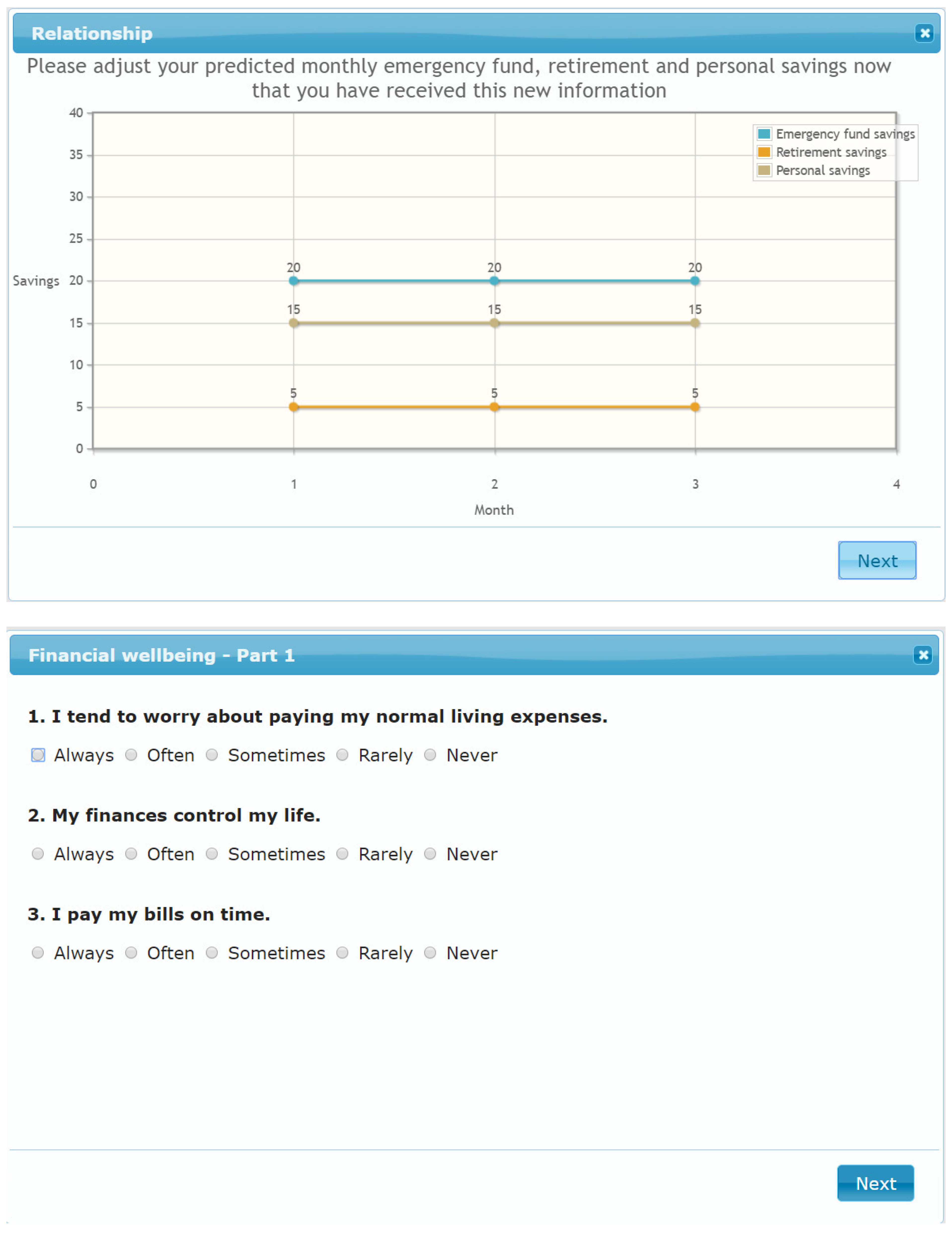
After reading the scenarios, participants were asked to rate the likelihood that this scenario would happen to them and how impactful they deem this would be on their financial situation. After rating the likelihood and the impact of the scenario, participants were presented with graphs of their forecasts and were asked to make any adjustments to their forecast they considered appropriate in light of the potential risk-related scenario they were given. This adjustment could be made by simply dragging the graph up or down, providing an easy way for the participant to visualize their expenses and savings. The first graph asked for an adjustment of the expenses, the second graph for the target savings and estimated savings, and the third graph for the three categories of savings. After these graphical adjustments, participants were asked to rate a few statements about financial wellbeing and financial literacy. Financial literacy and wellbeing are potentially important identifiers for understanding people’s financial forecasts and responses to risk information, and are further discussed in the Measures section below. Finally, participants were thanked for their participation and re-directed to the Prolific Academic website.
3.4. Variables and Measures
The following variables were measured in this study: (1) Predicted expenses, target savings, predicted savings and categories of savings; (2) Likelihood and impact of scenario; (3) Adjusted predictions; (4) Financial wellbeing; and (5) Financial literacy.
3.4.1. Predicted Expenses, Target Savings, Predicted Savings and Categories of Savings
These are surveyed using the following questions: (1) Target savings: how much do you want to save over the course of the following three months? (2) Predicted savings: how much do you think you will realistically save over the course of the following three months? (3) Predicted expenses: how much do you think you will realistically spend over the course of the following three months? (4) Categories of savings: “In general, savings can be divided into three categories: emergency fund savings, retirement savings, and personal savings. Please indicate how much you predict to save for each category over the course of the next three months.” The answers were measured via text input (numbers).
3.4.2. Likelihood and Impact of Scenario
After reading the scenario, participants were immediately asked for the likelihood and impact of the scenario via the following questions: (1) How likely do you deem this scenario to happen to you? (2) How impactful would this scenario be on your financial situation? The response scales are Likert scales ranging from 1 to 5, with 1 being ‘Not likely at all’ and ‘Not impactful’ respectively, and 5 being ‘Very likely’ and ‘Very impactful’ respectively.
3.4.3. Adjusted Predictions
These are measured via the graphical interface: the values of the adjusted line graphs are recorded. A negative percentage change value signifies a downsizing of the estimate; 0 represents no change, while a positive value signifies increasing the initial estimate. Percentage change in predictions after receiving the risk information were computed with the formula:
[(Adjusted − initial)/initial] × 100
3.4.4. Financial Wellbeing
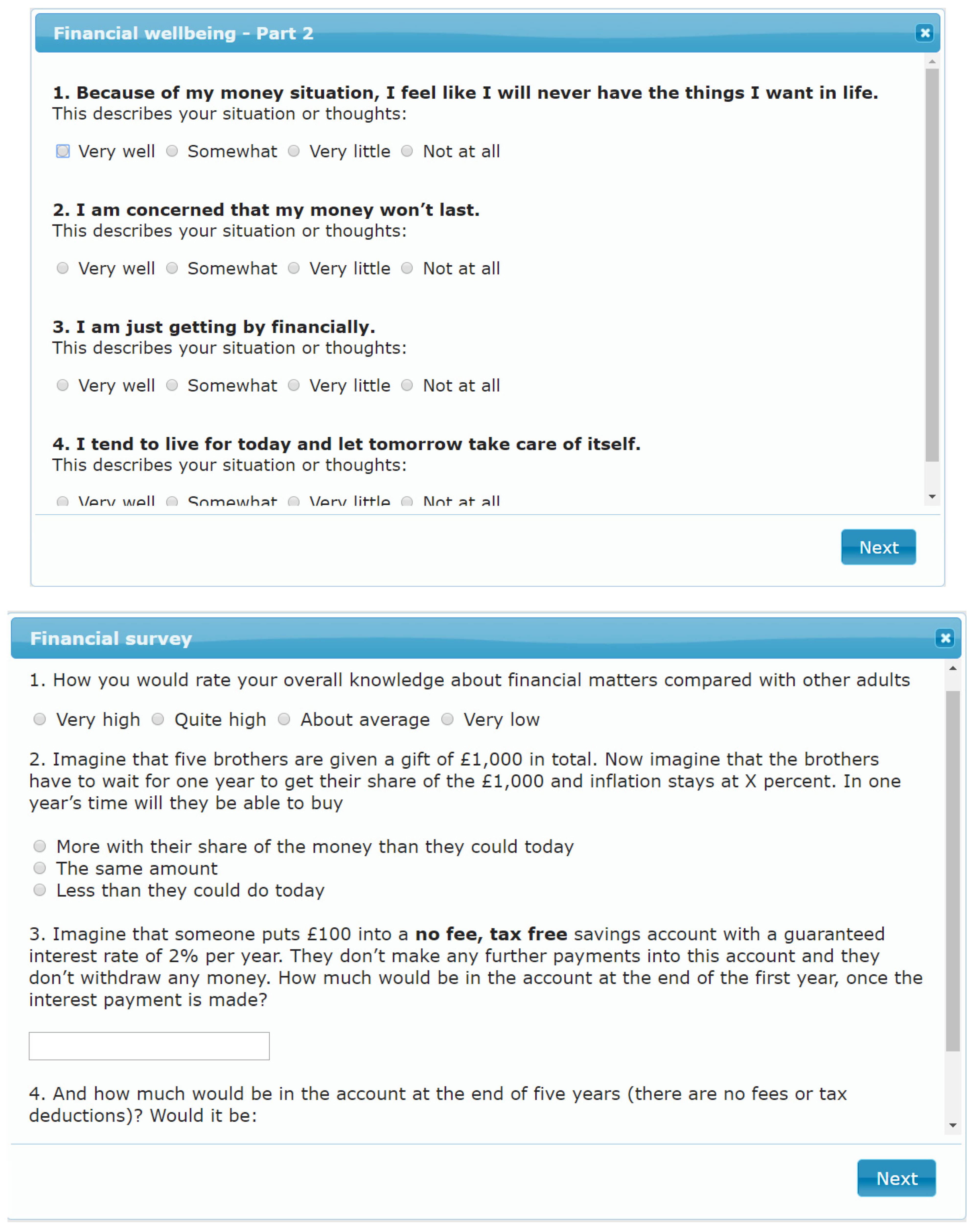
Financial wellbeing is a predictor of life satisfaction and health [70,71], and could potentially influence the base estimates in this study. This is measured via the OECD scale of financial wellbeing [72]. The first three items are answered on a 5-point Likert scale ranging from ‘Always’ to ‘Never’. These items are: (1) I tend to worry about paying my normal living expenses. (2) My finances control my life. (3) I pay my bills on time. The next four items are answered on a five-point Likert scale, with responses ranging from ‘Completely’ to ‘Not at all’. They are asked in how far the statement describes their situation or thoughts. (1) Because of my money situation, I feel like I will never have the things I want in life. (2) I am concerned that my money won’t last. (3) I am just getting by financially. (4) I tend to live for today and let tomorrow take care of itself.
3.4.5. Financial Literacy
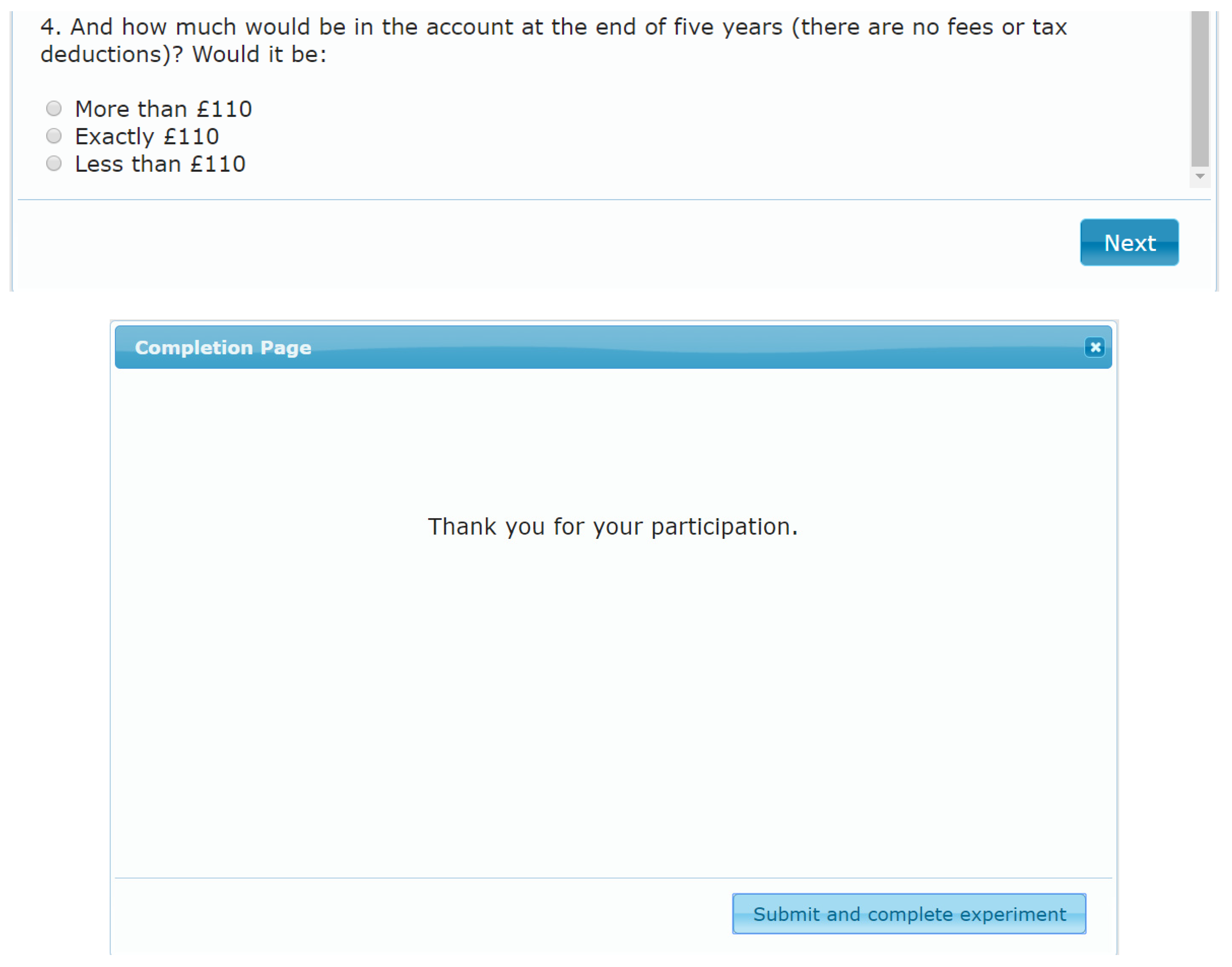
Financial literacy is linked to economic behaviour. There is, for instance, a positive relationship between financial literacy and planning for retirement [73]. Financial literacy is measured via the OECD scale of financial literacy [72]. Four items of this scale that are appropriate for our target audience were selected. The first item is a self-assessment, while the other three items are a knowledge test. (1) Self-assessment: “How you would rate your overall knowledge about financial matters compared with other adults?” The answering scale is a four-point Likert scale ranging from ‘Very high’ to ‘Very low’. (2) Knowledge test item 1: Imagine that five brothers are given a gift of £1000 in total. Now imagine that the brothers have to wait for one year to get their share of the £1000 and inflation stays at X percent. In one year’s time will they be able to buy: (a) more with their share of the money than they could today; (b) the same amount; (c) less than they could today. The correct response here is item C. (3) Knowledge test item 2: Imagine that someone puts £100 into a no fee, tax-free savings account with a guaranteed interest rate of 2% per year. They don’t make any further payments into this account, and they don’t withdraw any money. How much would be in the account at the end of the first year once the interest payment is made? (open-ended question, text input). The correct response here is £102. (4) Knowledge test item 3: And how much would be in the account at the end of five years (there are no fees or tax deductions)? Would it be: (a) More than £110; (b) Exactly £110; (c) Less than £110? The correct response here is option A.
4. Results
Given the experimental setup, this section first summarizes the findings from our exploratory analysis regarding participants’ perceptions of scenarios (in terms of likelihood and impact), followed by the analysis of experimental results and tests of our hypotheses.
4.1. Exploratory Analysis
4.1.1. Experimental Conditions Perception Check
Participants found the scenarios potentially likely and impactful. The mean likelihood of the scenarios can be found in Table 2 (Column 3). There were no significant differences among the conditions in either scenario (E (2164) = 0.60, p = 0.552; IL (2155) = 0.53, p = 0.721). The impact of the high-risk scenario was 4.14 (SD = 1.10), while the low-risk scenario was 3.68 (SD = 1.16), and the no-risk scenario was 3.02 (SD = 1.37): participants perceived clear differences between the impact for the three risk conditions (FRISK(2322) = 23.72, p < 0.001). A Tukey’s B post-hoc analysis shows that the high-risk group is significantly different from the low-risk group, which is in turn significantly different from the no-risk group.
4.1.2. Role of Background Variables
The financial wellbeing scale had a mean score of 3.26 (SD = 0.68), which is significantly different from the midpoint of the Likert scale (t(324) = 6.74, p < 0.001), indicating that people consider their financial wellbeing as better than average. The financial knowledge scale had a mean score for the self-assessment question of 2.30 (SD = 0.77). Participants assess themselves between the points ‘About average’ and ‘Quite high’. This score is significantly different from the midpoint of the scale (t(324) = −4.18, p < 0.001)—thus, we can say that people consider their financial knowledge to be slightly below average. The performance part consisted of three questions which could be answered right or wrong. Participants thus could achieve a maximum score of 3 out of 3. The mean score was 1.97 (SD = 0.86); this is significantly different from a 50% chance score (i.e., t-test compared with 1.5: (t(324) = 9.92, p < 0.001)), indicating a reasonably good performance on the knowledge test.
Interestingly, while our findings show no significant relationship of financial wellbeing and literacy scores to changes in forecasts in response to risk information, both the Financial Wellbeing and the Self-Assessed Financial Literacy seem to be correlated to predicted expenses, predicted savings (and savings subcategories) as well as to target savings (as given in Table A1, Appendix B). Thus, financial wellbeing and financial literacy play a role in the initial forecast value. However, as this study focuses on adjustment behaviour and these correlations are not significant, we do not take the measures further into account as control variables for our hypothesis testing.
4.2. Experimental Analyses
Table A2 shows the means and standard deviations for percentage changes for all the experimental variables. Adjustments in predicted expenses, predicted savings, target savings, savings categories, as well as no adjustment situations (Table A2; column 1) were examined via hypothesis testing, taking into account scenario context (unexpected expense or unexpected income loss; Table A2; column 2) and risk level (high risk, low risk or no risk; Table A2; column 3).
For the analysis of the results, we report the hypotheses below. These are grouped along the experimental setup’s two main variables: the scenario (with two levels, being either income loss or unexpected expenses) and the risk level (with three levels, being either zero, low, or high).
4.2.1. Scenarios
Hypothesis 1 predicted that savings forecasts will be adjusted downward for individuals receiving an unexpected income-loss scenario. To test this hypothesis, we performed a one-sided one-sample t-test, to test the assumption that the adjustments are negative. This turned out to be insignificant, both for target savings (t(157) = −1.35, p = 0.090) and predicted savings (t(157) = 0.801, p = 0.212). Thus, Hypothesis 1 is not confirmed.
Hypothesis 2 predicted that expense forecasts will be adjusted upward for individuals receiving the unexpected-expense scenario. Similarly, we performed a one-sided one-sample t-test to test the assumption that adjustments are positive. The t-test confirmed that the adjustments were positive (M = 9.14, SD = 29.65) and significantly different from 0 (t(166) = 3984, p < 0.001). Hypothesis 2 is confirmed.
4.2.2. Risk
Hypotheses 3–5 relate to the adjustments in light of the risk level. Hypothesis 3 stated that individuals receiving high-risk scenarios will make larger forecast adjustments than those receiving low-risk scenarios. To test this hypothesis, a one-sided independent samples t-test was run on the total absolute adjustment sizes (regardless of scenario content) in the high-risk condition versus those in the low-risk condition. The difference in adjustment size was not significantly larger in the high-risk condition (M = 24.69, SD = 21.71) than in the low-risk condition (M = 21.01, SD = 23.29; t(215) = −1.21, p = 0.115). Hypothesis 3 is thus not confirmed. Hypothesis 4 similarly stated that individuals receiving low-risk scenarios will make larger forecast adjustments than those receiving no-risk scenarios. A one-sided independent samples t-test shows that this is however not the case (t(214) = −0.31, p = 0.380), with the average adjustment size for the no-risk condition (M = 19.43, SD = 48.48) not being significantly different from the low-risk condition (M = 21.01, SD = 23.29). Hypothesis 4 is thus not confirmed. To delve deeper into these unexpected insignificant results, we ran further analyses to check whether the results of H3 and H4 are influenced by the scenario at hand (income loss versus unexpected expense), or the type of forecast (savings versus expenses). As in the t-tests above, we focus on the absolute values of the adjustments, as we are interested in investigating the hypotheses around adjustment size further, not adjustment direction.
First, we ran a two (scenario context) × three (risk level) two-way ANOVA on target savings adjustment sizes. This analysis indicates no main effect of scenario (FSCENARIO(1319) = 2.52, p = 0.113), a main effect of risk (FRISK(1319) = 6.02, p = 0.003), and no significant interaction effect (FSCENARIO×RISK(2319) = 1.69, p = 0.187). A Tukey’s B post hoc analysis for the significant main effect indicates that the adjustment size for target savings in the zero-risk scenario (M = 7.25, SD = 17.58) is significantly different (p < 0.05) from the low-risk (M = 14.44, SD = 24.00) and high-risk (M = 18.01, SD = 27.34) scenario, but the latter two are not significantly different from each other. Next, we ran a two (scenario context) × three (risk level) two-way ANOVA on predicted savings adjustment sizes. This analysis indicates no significant effects of scenario (FSCENARIO(1319) = 2.95, p = 0.087), nor risk (FRISK(1319) = 0.17, p = 0.845), nor an interaction effect (FSCENARIO×RISK(2319) = 0.71, p = 0.493). Last, we ran a 2 (scenario context) × 3 (risk level) two-way ANOVA on predicted expenses adjustment sizes. This analysis indicates no main effect of scenario (FSCENARIO(1319) = 1.61, p = 0.206), nor a main effect of risk (FRISK(1319) = 0.15, p = 0.865). However, a significant interaction effect was found (FSCENARIO×RISK(2319) = 3.44, p = 0.033). A simple effect analysis for this interaction effect shows a significant effect of scenario in the zero-risk condition (F(1319) = 6.82, p = 0.009), such that the expense scenario leads to an average adjustment size of 9.19 (SD = 11.46), while the income-loss scenario leads to an average adjustment size of 30.87 (SD = 92.55). Looking back at the adjustment size hypotheses (H3: high riskadjustment size > low riskadjustment size; H4: low riskadjustment size > no riskadjustment size), we note that H3 never holds, and H4 holds only in the target savings category.
Finally, Hypothesis 5 stated that the proportion of individuals in the no-risk condition that do not adjust their forecasts will be higher than those in the low-risk and high-risk conditions. To test this hypothesis, we first created a binomial variable no change/change, based on the adjustment sizes. If the adjustment size was anything other than 0, this was recoded as value 1. The proportion of people who did not change their input is displayed according to risk level, scenario, and output variable in Table A3 in Appendix B. For Hypothesis 5, we focus on the total proportion of ‘no-changers’ in the conditions according to the three risk levels, being 56.17% ‘no-changers’ in the zero-risk condition, 43.52% in the low-risk condition and 39.20% in the high-risk condition. A Kruskal-Wallis test indicates that these proportions are significantly different from each other (H(2) = 21.01, p < 0.001). Mann-Whitney pairwise comparisons indicate a significant difference between the zero-risk and the low-risk condition (U = 45,846, z = −3.22, p < 0.001), and between the zero-risk and high-risk condition (U = 43,791, z = −4.43, p < 0.001), but not between the low-risk and the high-risk condition (U = 50,494.50, z = −1.21, p = 0.225).
4.2.3. Categories of Savings
Hypothesis 6 posited that the sum of the three savings category forecasts will be more than the general category of predicted savings.
Examining the breakdowns into subcategories of savings (i.e., emergency fund savings, retirement savings and personal savings), we find that the breakdowns lead to lower total savings than the general savings forecasts. In particular, when the savings subcategories are summed, this sum of components differs significantly from the overall predicted savings (t(324) = −2.41; p = 0.016), with the summed total leading to a higher savings estimate (M = 709.08, SD = 1877.97) than the overall savings forecast (M = 524.47, SD = 1447.78). This confirms Hypothesis 6.
Hypothesis 7, relating back to the overoptimism effect in financial forecasts, stated that the estimates for the target savings category will be higher than those of the expected savings category. The forecasts for target savings are (M = 659.61, SD = 1362.96) indeed significantly higher than the predicted savings (M = 524.47, SD = 1447.78; t(324) = −4.6; p < 0.001). This confirms Hypothesis 7.
Additional Analyses
While not hypothesized, an interesting avenue for exploration is the effect of the category names or savings goals in our study. Given that we do not hypothesize a specific direction, and results are between-subjects, we ran two-sized paired samples t-tests on the means of the initial category estimations, and the mean changes (Table 3). An exploration of these means points towards two interesting findings regarding the retirement savings category. First, the initial retirement savings estimate is lowest of all, with a mean of 161.29 (SD = 692.77), significantly different from the initial estimate of the emergency fund savings with a mean of 257.59 (SD = 874.47; t(324) = 2.55, p = 0.011) and that of the personal savings with a mean of 290.19 (SD = 721.54; t(324) = −3.12, p = 0.002). However, the retirement savings category is at the same time adjusted the least, with an average adjustment size of 4.30 (SD = 15.61) in comparison with the emergency fund’s average adjustment of 19.64 (SD = 62.80; t(324) = 4.38, p < 0.001) and the personal savings’ adjustment size of 19.16 (SD = 44.91; t(324) = −5.94, p < 0.001). The emergency fund and personal savings do not differ significantly in initial estimate (t(324) = −0.68, p = 0.498) or in adjustment size (t(324) = 0.12, p = 0.905).
Another interesting takeaway from the savings categories can be found in the average adjustment direction. In reaction to the scenarios, the emergency fund savings are adjusted upwards, the retirement savings slightly downwards and the personal savings also downwards. Thus, in reaction to the scenarios containing risk, people seem to make a shift from personal savings towards emergency fund savings.
5. Discussion
We set up a study to investigate financial forecasting behaviour on a household or personal level. Many people do not have the necessary savings to account for unexpected expenditures and income loss [1,2,3]. A number of factors complicate decision making surrounding financial aspects: biases such as present bias, hyperbolic discounting, and overoptimism skew financial forecasts. One way to mediate the damaging effect of these biases is by using nudges. More specifically, this study looked at eliciting implementation intentions and precommitment strategies as ways of making information more salient and making forecasts more realistic. We set up an experimental study with scenarios (designed by means of a pilot study) where we varied the scenario frame (being either an income-loss scenario or an unexpected-expense scenario) and the risk level (zero, low, high). Outcome measures included predicted savings and expenses. The former was either formulated as target savings (goals) or predicted savings (forecasts), and divided into three categories: retirement savings, emergency fund savings, and personal savings.
5.1. Discussion of Results
5.1.1. Scenarios
Hypothesis 1 predicted that savings forecasts will be adjusted downward for individuals receiving an unexpected income-loss scenario. This was hypothesized based on the relationship found between income and savings in Brounen, Koedijk, and Pownall [55]. In a similar vein, Hypothesis 2 predicted that expense forecasts will be adjusted upward for individuals receiving the unexpected-expense scenario. Surprisingly, only in the unexpected-expense scenario did we notice the hypothesized effect (an upward adjustment of expected expenses); we did not find a downward adjustment of savings. This may be explained by salience: the effectiveness of the expense scenario in making the unexpected expenses more salient, thus leading to the observed upsurge in expense forecasts, but that the salience of the income category does not transfer to the savings category, as was originally found by Brounen et al. [55].
5.1.2. Risk
In our study, participants were assigned to three possible conditions: scenarios with high risk, low risk, or no risk. What was the effect of varying risk? Hypothesis 3 and 4, respectively, predicted that a higher risk displayed in the scenario would lead to a larger average adjustment size. More concretely, zero-risk adjustment sizes were predicted to be smaller than low-risk adjustment sizes, which in turn were predicted to be lower than high-risk adjustment sizes. Surprisingly, adjustments did not differ significantly across risk levels. However, we noted in the analysis section that we did not distinguish according to scenario nor output variable, following earlier results of [56]. We therefore dug deeper, taking scenario (income loss versus unexpected expense) and outcome variable (expenses versus savings; target or predicted savings) into account. Notably, the adjustment sizes from Hypothesis 3, comparing high-risk and low-risk scenarios, were never significant, even when accounting for scenario type or output variable (predicted expenses, target savings, predicted savings). Hypothesis 4, comparing the zero-risk to the low-risk category, only holds for target savings. This lack of consistent effect of risk size was unexpected. It is not that participants did not adjust their estimates; they did, but they all did it in a fairly consistent manner, despite the frame and risk level.
To dig further into the absence of this risk effect, we looked at the results of Hypothesis 5, which related to the proportion of people who did not change their forecasts. Logic dictates that the proportion of people in the zero-risk condition who did not change their forecasts would be significantly more than those in the low-risk condition, which in turn would be more than in the high-risk condition. A prevalent finding in forecasting research is that people adjust insufficiently or not at all (often due to status quo bias or omission bias; [57]). This study indeed found that a higher percentage of participants receiving the zero-risk scenario did not alter their forecast compared to the low-risk condition and the high-risk condition. An interesting note should be made of the fact that the proportion of people who did not change in the zero-risk condition was not 100%. On the contrary, more than half made changes despite not having a particular reason to do so. Why would being faced with the zero-risk scenario still elicit behaviour change? A possibility could be the mere exposure effect: the scenario is read and while not having an effect, it still increases the salience that such a thing may happen in the future. One could term it as a ‘lucky break’ effect: people read about something negative and impactful that could have happened to them, but it did not. Such a near-miss may be perceived as being given a lucky break this time around, but who knows what could happen next time. This result suggests interesting avenues for future nudging research, in that providing information can elicit behavioural changes simply by increasing the salience of the financial risk.
5.1.3. Categories of Savings
This study found, as hypothesized, that the breakdown of savings into subcategories of savings led to a higher total savings amount. Labelling money for a specific purpose, or ‘earmarking’ it has been known to increase savings. Soman and Cheema [62] found that people saved more when money was partitioned into two different accounts than when it was pooled into one account. This relates back to the concept of mental accounting, which implies that people designate certain amounts of money to specific purposes [74]. Our study asked people to provide an overall prediction for their savings, as well as for three different subcategories: savings for an emergency fund, retirement savings and personal savings. Interestingly, it is found that when all the categories are summated, the total estimate is higher than the overall savings forecast. This is in line with the Savings Goals Theory and mental budgeting literature cited above (e.g., [61]). Mental accounting, decision bracketing, or ‘narrow framing’ are all interconnected and relate to the phenomenon that more narrowly framed decisions or categories are more ‘acceptable’, or more salient, than a wider category [75]. Thus, as a takeaway, if we want to nudge people towards increasing their savings, we need to encourage them to make projections for different savings subcategories. While not hypothesized, a finding of note is that the retirement savings category had the lowest initial estimate to start with; yet was also the least adjusted. This result is a somewhat mixed message. Surveys have shown that a large part of the population does not have sufficient retirement savings in their name [20], and the empirical results corroborate that retirement savings do not appear to take priority over other subcategories. However, when an unexpected financial shock is brought to their attention, people adjusted the retirement savings category only minimally. Further research should explore the motivation behind this more. It is possible that government encouragement and awareness strategies have had a positive effect on people’s financial awareness regarding retirement savings. It is a positive evolution that retirement savings seem to hold steady through turmoil, yet the question remains why it is estimated lower, compared to, for instance, personal savings. An explanation here could be the time factor: for a large part of the population, ‘retirement’ is something that is far ahead in the future. The biases discussed in the literature section come back into play here: a present bias that makes us focus on the present or near future (and retirement being far away), or the hyperbolic discounting of Thaler [26], could lead retirement to be seen as a vague concept in a long-term future perspective. Additionally, regarding savings categories, potential further research could split up the ‘personal savings’ category further, and look at savings motivational goals [65] as a potential exploratory factor. Another effect of note, which was not hypothesized, is the direction of the adjustments in three savings categories: retirement funds are barely adjusted (slightly downwards), personal savings are adjusted significantly downwards, and emergency fund savings significantly upwards. Thus, it seems that an interchange happens between the allocation of savings from the personal category to the emergency fund category. Presumably, the described scenarios elicited a wider range of potential risk, leading people to save more for these types of risks than for personal, potentially more frivolous sources (e.g., travel). This points towards yet another reason to consider splitting up personal savings along motivational categories in future research.
Furthermore, we looked at the effect of word usage in eliciting forecasts. ’Target’ savings predications were higher than the ’predicted savings’ category: people set targets, but when asked to make a realistic assessment, they estimate them lower than their targeted amounts. A number of factors could play a role here. It is possible that the word ‘target’ elicits an overoptimistic response, while ‘prediction’ leads to a lower and perhaps more realistic estimation. It could be that people initially set the bar a bit higher due to a desirability bias; they start with a higher (more desirable) ‘anchor’ in the hope that this will translate to increased actual savings. If we want to nudge people towards higher savings, we could potentially benefit from advocating a focus on targets, as emphasized previously. An important theory here is goal setting theory [76], which showed that specific, high goals lead to higher performance than vague, abstract goals. Presumably, the target savings category was seen as a higher goal than a predicted savings category, with the latter stressing ‘realistically’. However, more research into the specific framework of goal setting theory is needed to further this theory. This ‘target’ formulation can also be seen as a type of nudge falling under eliciting implementation intentions and precommitment [45]. This is a new way of achieving the effect found by Thaler and Benartzi’s [30] Save More Tomorrow (SMART) program, which focused on another type of nudge: the design of choice architecture (the opt-out instead of opt-in approach for an employee’s retirement savings to increase retirement savings). Thus, there may be a linguistic effect of using the word ‘target’ versus ‘prediction’, which forms a potential avenue for future research.
5.1.4. Limitations and Directions for Future Research
While leading to important behavioural insights into individuals’ forecasts of savings and expenses and their reactions to scenarios with various risk levels, the current work also has limitations that could be addressed with future studies. One such limitation is social desirability, which can be examined by using a full-factorial between-subjects design. In the current study, participants did not see both high- and low-risk scenarios, for instance, thereby obscuring the vital role of the scenario’s riskiness. Each participant was exposed only to one scenario context with a single risk level. Further scenario contexts employed in conjunction with a full spectrum of risk levels could yield enhanced insights into people’s responses to varying contexts and risk levels. Additionally, this experiment used a varied sample from the crowdsourcing platform Prolific Academic. Such online samples can provide a greater variety of data than what can be obtained in a simple laboratory experiment. Online experimental platforms are easy to use, are low cost and provide a more heterogeneous sample than the commonly used student sample [77,78,79,80]. Online experiments may also reduce social desirability and similar expectancy effects [81] as the participants’ identities are unknown and there are no real-life consequences. It would be interesting to conduct similar experiments in behavioural laboratory settings with more homogeneous samples in highly controlled environments.
A natural extension of the current work is to ask for expense targets as well as forecasts of expense subcategories, as was currently done with savings targets and forecasts for savings subcategories. Additionally, future research could examine the connection with temporal dispositions such as a time perspective, planning behaviour or the delay of gratification. Scales of interest include the brief time perspective scale, which measures future/present orientation [82], the propensity to plan scale, which measures planning behaviour [83], or the monetary choice questionnaire, which measures preference for immediate or delayed rewards [84]. According to resource slack theory [27] and construal level theory [29], people are overoptimistic about the resources they will have available to them in the future, but are less so in the time frame nearer to the decision making period. Using various time frames to elicit forecasts may yield clues about how to better support their financial planning. In this study, while time frames were not central to its theorizing, participants were asked to provide estimates for the following three months. The further away people were asked to forecast, the higher their savings estimates became. Estimates of expenses, however, remained quite steady. This was, however, not the initial goal of our research, and an avenue for further study is varying the time horizon, not only by a matter of months, but also by days, weeks or years.
Future research could add more variables of interest in line with our choice of financial literacy and financial wellbeing: dispositional factors such as risk propensity and long-term orientation have been found to play a role in financial behaviour (e.g., [85]), as well as situational factors such as, for instance, uncertainty, most recently that which was triggered by the pandemic (e.g., [86]).
An important note in nudging research should be made about the ethical aspects of influencing people’s behaviour [45]. Nudges should never venture into the realm of manipulation, but should be open and transparent [45]. We therefore opted for scenarios that provide information, and formulated questions towards intended future financial behaviour. As such, this type of nudging falls under eliciting implementation intentions and precommitment strategies [45].
Further insights into current findings could be gleaned from treating the varying risk levels used in the current study as risk-to-self versus risk-to-others. From this perspective, the high-risk and low-risk scenarios would constitute plausible situations where the risk information is directly relevant and applicable to self; whereas the no-risk scenario could be perceived as a setting where the risk happens to other people. As we found in this study, the latter may lead to what we have termed the ’lucky break’ effect—a near-miss situation where ‘it could have been me but wasn’t in this instance, but what if it is me next time’. Future studies to elicit people’s reactions to these situations would be very valuable in supporting designs of effective nudging tools.
It should be noted that this study took place right before the onset of the COVID-19 pandemic. A recommendation for future research would entail a repeat of this study either later during the pandemic or post pandemic to test for the stability of the findings in a world that has undergone significant change. However, regulations such as lockdowns and consequences of the disease (e.g., hospitalization rate) differ per country, leading to a wide range of conclusions and a need for a global study. For instance, Levine, Lin, Tai and Xie [87] found a relationship in the USA between COVID-19 infection ratings and reduced spending combined with increased saving. The investigated driver behind this behaviour is increased anxiety regarding potential job loss. In contrast, a study in Eastern Europe [86] found not an increase but a reduction in savings. Another factor investigated with regard to the pandemic that is of importance to this study is financial risk tolerance (FRT). FRT was found to have decreased during the first stages of the pandemic, mostly with young people [88]. Chhatwani and Mishra [89], however, note that FRT studies during the pandemic are limited, and that factors such as financial literacy can moderate the effect. Thus, much remains to be explored as the situation unfolds.
6. Conclusions
Many people are financially fragile in that they do not have the necessary monetary backups to deal with unexpected financial risk, such as the loss of income or an unexpected expense. Additionally, when people are requested to make household financial forecasts, they are subject to a wide range of biases. They are overoptimistic, leading to an underestimation of expenses and an overestimation of income. They are present-oriented and have difficulties correctly valuing financial risks that are further in the future. Therefore, this study set out to investigate whether we can aid people in their financial forecasts and nudge them in the right direction. We set up an experiment that investigated the influence of risk scenarios and investigated people’s forecasts before and after being made aware of certain risks. Forecasts were made on expenses and savings, and scenarios were either on unexpected expenses or on income loss, with three varying degrees of risk: none, low, or high. Surprisingly, even a scenario with no risk led to adjusting behaviour. We termed this the lucky break effect: it seems that the mere increased salience of a risk already triggers a change in financial forecasts. One is lucky to have escaped the risk and is now more aware of it. Additionally, we found that expense related scenarios had an effect on expense forecasts, but income related scenarios did not have an effect on savings forecasts. However, two other important factors with regard to savings forecasts were found: first, using the word ‘target savings’ rather than ‘predicted savings’ led to higher savings estimates (and one should hope, subsequent commitment to this higher savings target). Second, encouraging people to make forecasts according to different savings goals led to higher predicted savings compared to eliciting an overall savings prediction. With these results, we aim to aid governments and financial aid institutions in nudging people in the direction of more financial awareness (of expenses) and increased savings (via the use of targets and categorical savings).
Author Contributions
Conceptualization, D.Ö.; data curation, S.D.B.; formal analysis, S.D.B.; funding acquisition, S.D.B., D.Ö. and W.A.; investigation, S.D.B. and D.Ö.; methodology, S.D.B.; project administration, D.Ö.; resources, S.D.B.; software, S.D.B.; supervision, D.Ö.; validation, S.D.B.; visualization, S.D.B. and W.A.; writing—original draft, S.D.B. and D.Ö.; writing—review & editing, S.D.B., D.Ö. and W.A. All authors have read and agreed to the published version of the manuscript.
Funding
This research was funded by the ING Think Forward Initiative Short-Term Research Grant TFI-STP-2019_71 for all authors and by the Research Foundation Flanders (FWO) for the first author.
Institutional Review Board Statement
The study was conducted according to the guidelines of the Declaration of Helsinki, and approved by the Ethics Committee of NORTHUMBRIA UNIVERSITY (Reference number 15576, date of approval: 28 February 2019).
Informed Consent Statement
Informed consent was obtained from all subjects involved in the study.
Data Availability Statement
The data presented in this study are available on request from the corresponding author. The data are not publicly available due to a privacy agreement with the funding agency.
Conflicts of Interest
The authors declare that they have no conflict of interest.
Appendix A
Figure A1.
Screenshots of experiment.


Appendix B

Table A1.
Spearman’s rho correlations of financial wellbeing and financial literacy (as measured via Self-Assesment and Performance Score) on initial forecasts and percentage changes in forecasts (post-scenario).
Table A1.
Spearman’s rho correlations of financial wellbeing and financial literacy (as measured via Self-Assesment and Performance Score) on initial forecasts and percentage changes in forecasts (post-scenario).
| Financial Wellbeing | Financial Literacy (Self-Assessment) | Financial Literacy (Performance Score) | |
|---|---|---|---|
| PE | 0.150 ** (0.007) | 0.153 ** (0.006) | 0.226 ** (0.000) |
| PS | 0.320 ** (0.000) | 0.196 ** (0.000) | 0.065 (0.242) |
| TS | 0.235 ** (0.000) | 0.179 ** (0.001) | 0.064 (0.249) |
| EFS | 0.152 ** (0.006) | 0.186 ** (0.001) | −0.012 (0.826) |
| RS | 0.130 * (0.019) | 0.105 (0.058) | −0.041 (0.456) |
| PerS | 0.258 ** (0.000) | 0.140 * (0.012) | 0.028 (0.619) |
| PE %change | −0.059 (0.290) | 0.057 (0.308) | 0.031 (0.577) |
| PS %change | 0.073 (0.187) | −0.008 (0.891) | −0.020 (0.719) |
| TS %change | 0.092 (0.097) | 0.025 (0.650) | 0.010 (0.853) |
| EFS %change | 0.007 (0.897) | 0.017 (0.762) | −0.030 (0.586) |
| RS %change | 0.053 (0.343) | 0.011 (0.849) | −0.028 (0.620) |
| PerS %change | −0.051 (0.362) | 0.100 (0.070) | −0.060 (0.279) |
* p < 0.05; ** p < 0.01 [2-tailed p-values in parenthesis]; PE = Predicted Expenses; TS = Target Savings: PS = Predicted Savings; EFS = Emergency Fund Savings; RS = Retirement Savings; PerS = Personal Savings.
Table A2.
Means and SD’s of the dependent variables across scenario context and risk level.
| Scenario Context | Risk Level | Mean | SD | n | |
|---|---|---|---|---|---|
| Predicted Expenses (%change) | Expense | No risk | 2.61 | 14.50 | 54 |
| Low risk | 14.54 | 34.18 | 56 | ||
| High risk | 10.02 | 34.47 | 57 | ||
| Income Loss | No risk | −4.49 | 97.55 | 54 | |
| Low risk | −21.03 | 27.56 | 52 | ||
| High risk | −15.40 | 21.91 | 52 | ||
| Target Savings (%change) | Expense | No risk | 1.90 | 14.00 | 54 |
| Low risk | −8.50 | 22.62 | 56 | ||
| High risk | −15.87 | 28.94 | 57 | ||
| Income Loss | No risk | −5.59 | 22.36 | 54 | |
| Low risk | 0.58 | 31.91 | 52 | ||
| High risk | −4.27 | 32.50 | 52 | ||
| Predicted Savings (%change) | Expense | No risk | 6.59 | 55.23 | 54 |
| Low risk | −5.01 | 30.46 | 56 | ||
| High risk | −30.51 | 35.27 | 57 | ||
| Income Loss | No risk | 15.29 | 157.18 | 54 | |
| Low risk | 5.68 | 59.11 | 52 | ||
| High risk | −1.76 | 53.66 | 52 | ||
| Predicted Emergency Funds Savings (%change) | Expense | No risk | 3.82 | 30.42 | 54 |
| Low risk | 5.88 | 32.43 | 56 | ||
| High risk | 7.70 | 114.65 | 57 | ||
| Income Loss | No risk | 2.87 | 32.92 | 54 | |
| Low risk | 14.14 | 87.79 | 52 | ||
| High risk | 11.28 | 41.04 | 52 | ||
| Predicted Retirement Savings (%change) | Expense | No risk | −2.04 | 10.62 | 54 |
| Low risk | 0.51 | 7.07 | 56 | ||
| High risk | −3.46 | 14.16 | 57 | ||
| Income Loss | No risk | −2.93 | 18.55 | 54 | |
| Low risk | −1.61 | 18.97 | 52 | ||
| High risk | −2.53 | 22.83 | 52 | ||
| Predicted Personal Savings (%change) | Expense | No risk | −2.12 | 16.73 | 54 |
| Low risk | −9.06 | 20.37 | 56 | ||
| High risk | −18.21 | 36.62 | 57 | ||
| Income Loss | No risk | −3.28 | 42.18 | 54 | |
| Low risk | 3.55 | 95.99 | 52 | ||
| High risk | −10.58 | 35.75 | 52 |
Table A3.
Proportion of people who don’t change their input.
| Risk Level | Scenario | Output Variable | Proportion No Change (n (% Total of Scenario)) |
|---|---|---|---|
| Zero risk | Income loss | Target Savings | 37 (68.50%) |
| Predicted Savings | 28 (51.90%) | ||
| Predicted Expenses | 20 (37.00%) | ||
| Expenses | Target Savings | 43 (79.60%) | |
| Predicted Savings | 29 (53.70%) | ||
| Predicted Expenses | 25 (46.30%) | ||
| Low risk | Income loss | Target Savings | 21 (40.40%) |
| Predicted Savings | 20 (38.50%) | ||
| Predicted Expenses | 17 (32.70%) | ||
| Expenses | Target Savings | 38 (67.90%) | |
| Predicted Savings | 28 (50.00%) | ||
| Predicted Expenses | 17 (30.40%) | ||
| High risk | Income loss | Target Savings | 31 (59.60%) |
| Predicted Savings | 21 (40.40%) | ||
| Predicted Expenses | 14 (26.90%) | ||
| Expenses | Target Savings | 31 (54.4%) | |
| Predicted Savings | 19 (33.33%) | ||
| Predicted Expenses | 11 (19.30%) |
References
- Grinstein-Weiss, M.; Russell, B.D.; Gale, W.G.; Key, C.; Ariely, D. Behavioral Interventions to Increase Tax-Time Saving: Evidence from a National Randomized Trial. J. Consum. Aff. 2017, 51, 3–26. [Google Scholar] [CrossRef]
- Hogarth, J.M.; Anguelov, C.E.; Lee, J. Can the poor save? J. Financ. Couns. Plan. 2003, 14, 1–18. [Google Scholar]
- Lusardi, A.; Schneider, D.J.; Tufano, P. Financially Fragile Households: Evidence and Implications. Available online: https://www.nber.org/papers/w17072 (accessed on 11 July 2021).
- Weller, C.E.; Logan, A.M. Measuring Middle Class Economic Security. J. Econ. Issues 2009, 43, 327–336. [Google Scholar] [CrossRef]
- Frederick, S.; Loewenstein, G.; O’Donoghue, T. Time Discounting and Time Preference: A Critical Review. J. Econ. Lit. 2002, 40, 351–401. [Google Scholar] [CrossRef]
- Tam, L.; Dholakia, U.M. Delay and duration effects of time frames on personal savings estimates and behavior. Organ. Behav. Hum. Decis. Processes 2011, 114, 142–152. [Google Scholar] [CrossRef]
- Ainslie, G. Picoeconomics; Cambridge University Press: Cambridge, UK, 1992. [Google Scholar]
- Angeletos, G.-M.; Laibson, D.; Repetto, A.; Tobacman, J.; Weinberg, S. The Hyperbolic Consumption Model: Calibration, Simulation, and Empirical Evaluation. J. Econ. Perspect. 2001, 15, 47–68. [Google Scholar] [CrossRef] [Green Version]
- O’Donoghue, T.; Rabin, M. Doing it now or later. Am. Econ. Rev. 1999, 89, 103–124. [Google Scholar] [CrossRef] [Green Version]
- Howard, C.; Hardisty, D.; Sussman, A.; Knoll, M. Understanding the expense prediction bias. In Advances in Consumer Research; Moreau, P., Puntoni, S., Eds.; Association for Consumer Research: Duluth, MN, USA, 2016; Volume 44, pp. 190–194. [Google Scholar]
- Weinstein, N.D.; Klein, W.M. Unrealistic Optimism: Present and Future. J. Soc. Clin. Psychol. 1996, 15, 1–8. [Google Scholar] [CrossRef]
- Newby-Clark, I.R.; Ross, M. Conceiving the Past and Future. Pers. And Soc. Psy. Bull. 2003, 29, 807–818. [Google Scholar] [CrossRef]
- Thaler, R.; Sunstein, C.R. Behavioral economics, public policy and paternalism: Libertarian paternalism. Am. Econ. Rev. 2003, 93, 175–179. [Google Scholar] [CrossRef] [Green Version]
- Ratner, R.K.; Soman, D.; Zauberman, G.; Ariely, D.; Carmon, Z.; Keller, P.A.; Kim, B.K.; Lin, F.; Malkoc, S.; Small, D.A.; et al. How behavioral decision research can enhance consumer welfare: From freedom of choice to paternalistic intervention. Mark. Lett. 2008, 19, 383–397. [Google Scholar] [CrossRef]
- Johnson, E.J.; Shu, S.B.; Dellaert, B.G.C.; Fox, C.; Goldstein, D.G.; Häubl, G.; Larrick, R.P.; Payne, J.W.; Peters, E.; Schkade, D.; et al. Beyond nudges: Tools of a choice architecture. Mark. Lett. 2012, 23, 487–504. [Google Scholar] [CrossRef]
- OECD. OECD Economic Outlook No. 94; OECD: Paris, France, 2013. [Google Scholar]
- Dugas, C. Retirement Crisis Looms as Many Come Up Short. USA Today. 19 July 2002. Available online: http://globalag.igc.org/pension/us/private/retirement.htm (accessed on 13 December 2021).
- Munnell, A.; Webb, A.; Delorme, L. Retirements at Risk: A New National Retirement Index; Center for Retirement Research at Boston College: Newton, MA, USA, June 2006. [Google Scholar]
- Collinson, P. One in three UK retirees will have to rely solely on state pension. The Guardian. 21 October 2017. Available online: https://www.theguardian.com/money/2017/oct/21/uk-retirees-state-pension-financial-future (accessed on 13 December 2021).
- Benartzi, S.; Thaler, R. Behavioral economics and the retirement savings crisis. Science 2013, 339, 1152–1153. [Google Scholar] [CrossRef] [PubMed]
- Nova, A. Americans need to double their retirement savings. CNBC 2018. Available online: https://www.cnbc.com/2018/11/13/most-americans-arent-saving-nearly-enough-for-retirement.html (accessed on 13 December 2021).
- Chartrand, T.L.; Huber, J.; Shiv, B.; Tanner, R.J. Nonconscious Goals and Consumer Choice. J. Consum. Res. 2008, 35, 189–201. [Google Scholar] [CrossRef]
- Sussman, A.B.; Alter, A.L. The Exception Is the Rule: Underestimating and Overspending on Exceptional Expenses. J. Consum. Res. 2012, 39, 800–814. [Google Scholar] [CrossRef]
- Loewenstein, G.; Prelec, D. Anomalies in intertemporal choice: Evidence and an interpretation. Q. J. Econ. 1992, 107, 573–597. [Google Scholar] [CrossRef]
- Read, D.; Scholten, M. Future-oriented decisions: Intertemporal choice. In Economic Psychology; Ranyard, R., Ed.; John Wiley & Sons: Hoboken, NJ, USA, 2018. [Google Scholar]
- Thaler, R. Some Empirical Evidence on Dynamic Inconsistency. Econ. Lett. 1981, 8, 201–207. [Google Scholar] [CrossRef]
- Zauberman, G.; Lynch, J.J.G. Resource slack and propensity to discount delayed investments of time versus money. J. Exp. Psychol. Gen. 2005, 134, 23–37. [Google Scholar] [CrossRef]
- Newby-Clark, I.R.; Ross, M.; Buehler, R.; Koehler, D.J.; Griffin, D. People focus on optimistic scenarios and disregard pessimistic scenarios while predicting task completion times. J. Exp. Psychol. Appl. 2000, 6, 171–182. [Google Scholar] [CrossRef]
- Liberman, N.; Trope, Y. The role of feasibility and desirability considerations in near and distant future decisions: A test of temporal construal theory. J. Personal. Soc. Psychol. 1998, 75, 5–18. [Google Scholar] [CrossRef]
- Thaler, R.H.; Benartzi, S. Save More Tomorrow (TM): Using behavioral economics to increase employee saving. J. Political Econ. 2004, 112, S164–S187. [Google Scholar] [CrossRef]
- Thaler, R.; Sunstein, C.R. Nudge: Improving Decisions about Health, Wealth and Happiness; Yale University Press: New Haven, CT, USA, 2008. [Google Scholar]
- Lofgren, A.; Nordblom, K. A theoretical framework of decision making explaining the mechanisms of nudging. J. Econ. Behav. Organ. 2020, 174, 1–12. [Google Scholar] [CrossRef]
- Gigerenzer, G.; Gaissmaier, W. Heuristic Decision Making. Annu. Rev. Psychol. 2011, 62, 451–482. [Google Scholar] [CrossRef] [PubMed] [Green Version]
- Tversky, A.; Kahneman, D. Judgment under uncertainty: Heuristics and biases. Science 1974, 185, 1124–1131. [Google Scholar] [CrossRef]
- Hummel, D.; Maedche, A. How effective is nudging? A quantitative review on the effect sizes and limits of empirical nudging studies. J. Behav. Exp. Econ. 2019, 80, 47–58. [Google Scholar] [CrossRef]
- Cadario, R.; Chandon, P. Which Healthy Eating Nudges Work Best? A Meta-Analysis of Field Experiments. Mark. Sci. 2020, 39, 465–486. [Google Scholar] [CrossRef]
- Chetty, R.; Friedman, J.N.; Leth-Petersen, S.; Nielsen, T.H.; Olsen, T. Subsidies vs. nudges: Which policies increase saving the most? Issue Brief 2013, 13, 7. [Google Scholar]
- García, J.M.; Vila, J. Financial literacy is not enough: The role of nudging toward adequate long-term saving behavior. J. Bus. Res. 2020, 112, 472–477. [Google Scholar] [CrossRef]
- Ebrahimi, O.V.; Hoffart, A.; Johnson, S.U. Viral mitigation and the COVID-19 pandemic: Factors associated with adherence to social distancing protocols and hygienic behaviour. Psychol. Health 2021, 1–24. [Google Scholar] [CrossRef]
- Renosa, M.D.C.; Landicho, J.; Wachinger, J.; Dalglish, S.L.; Barnighausen, K.; Barnighausen, T.; McMahon, S.A. Nudging toward vaccination: A systematic review. BMJ Glob. Health 2021, 6, e006237. [Google Scholar] [CrossRef] [PubMed]
- Weijers, R.J.; de Koning, B.B. Nudging to Increase Hand Hygiene during the COVID-19 Pandemic: A Field Experiment. Can. J. Behav. Sci. 2021, 53, 353–357. [Google Scholar] [CrossRef]
- Cardella, E.; Kalenkoski, C.M.; Parent, M. Less is not more: 401(k) plan information and retirement planning choices. J. Pension Econ. Financ. 2021, 1–21. [Google Scholar] [CrossRef]
- Medina, P.C. Side Effects of Nudging: Evidence from a Randomized Intervention in the Credit Card Market. Rev. Financ. Stud. 2021, 34, 2580–2607. [Google Scholar] [CrossRef]
- Hendy, P.; Slonim, R.; Atalay, K. Unsticking credit card repayments from the minimum: Advice, anchors and financial incentives. J. Behav. Exp. Financ. 2021, 30, 100505. [Google Scholar] [CrossRef]
- Sunstein, C.R. Nudging: A very short guide. Bus. Econ. 2019, 54, 127–129. [Google Scholar] [CrossRef]
- Onkal, D.; Sayim, K.Z.; Gonul, M.S. Scenarios as channels of forecast advice. Technol. Forecast. Soc. 2013, 80, 772–788. [Google Scholar] [CrossRef] [Green Version]
- Goodwin, P.; Gonul, M.S.; Onkal, D. When providing optimistic and pessimistic scenarios can be detrimental to judgmental demand forecasts and production decisions. Eur. J. Oper. Res. 2019, 273, 992–1004. [Google Scholar] [CrossRef]
- Fildes, R.; Goodwin, P.; Lawrence, M. The design features of forecasting support systems and their effectiveness. Decis. Support Syst. 2006, 42, 351–361. [Google Scholar] [CrossRef] [Green Version]
- Wright, G.; Goodwin, P. Decision making and planning under low levels of predictability: Enhancing the scenario method. Int. J. Forecast. 2009, 25, 813–825. [Google Scholar] [CrossRef] [Green Version]
- Satterfield, T.; Slovic, P.; Gregory, R. Narrative valuation in a policy judgment context. Ecol. Econ. 2000, 34, 315–331. [Google Scholar] [CrossRef]
- Goodwin, P.; Gönül, S.; Önkal, D.; Kocabıyıkoğlu, A.; Göğüş, C.I. Contrast effects in judgmental forecasting when assessing the implications of worst and best case scenarios. J. Behav. Decis. Mak. 2019, 32, 536–549. [Google Scholar] [CrossRef]
- Schoemaker, P.J.H. When and How to Use Scenario Planning—A Heuristic Approach with Illustration. J. Forecast. 1991, 10, 549–564. [Google Scholar] [CrossRef]
- Leika, M.; Marchettini, D. A Generalized Framework for the Assessment of Household Financial Vulnerability; International Monetary Fund: Washington, DC, USA, 2017. [Google Scholar]
- Christelis, D.; Jappelli, T.; Paccagnella, O.; Weber, G. Income, wealth and financial fragility in Europe. J. Eur. Soc. Policy 2009, 19, 359–376. [Google Scholar] [CrossRef]
- Brounen, D.; Koedijk, K.G.; Pownall, R.A.J. Household financial planning and savings behavior. J. Int. Money Financ. 2016, 69, 95–107. [Google Scholar] [CrossRef]
- Önkal, D.; Gönül, S.; Goodwin, P. Judgmental adjustments and scenario use: Individual versus group forecasts. In Proceedings of the ISF 2020: 40th International Symposium on Forecasting, Virtual, Rio de Janeiro, Brazil, 25 October 2020. [Google Scholar]
- Yaniv, I.; Schul, Y. Acceptance and elimination procedures in choice: Noncomplementarity and the role of implied status quo. Organ. Behav. Hum. Decis. Processes 2000, 82, 293–313. [Google Scholar] [CrossRef]
- Yaniv, I. The benefit of additional opinions. Curr. Dir. Psychol. Sci. 2004, 13, 75–78. [Google Scholar] [CrossRef] [Green Version]
- Keynes, J.M. The General Theory of Employment, Interest and Money; Macmillan: New York, NY, USA, 1936. [Google Scholar]
- Thaler, R.H. Mental accounting Matters. J. Behav. Decis. Mak. 1999, 12, 183–206. [Google Scholar] [CrossRef]
- Antonides, G.; de Groot, I.M.; van Raaij, W.F. Mental budgeting and the management of household finance. J. Econ. Psychol. 2011, 32, 546–555. [Google Scholar] [CrossRef]
- Soman, D.; Cheema, A. Earmarking and Partitioning: Increasing Saving by Low-Income Households. J. Mark. Res. 2011, 48, S14–S22. [Google Scholar] [CrossRef]
- Sussman, A.B.; O’Brien, R.L. Knowing When to Spend: Unintended Financial Consequences of Earmarking to Encourage Savings. J. Mark. Res. 2016, 53, 790–803. [Google Scholar] [CrossRef]
- Zhang, C.Y.; Sussman, A.B. Perspectives on mental accounting: An exploration of budgeting and investing. Financ. Plan. Rev. 2018, 1, e1011. [Google Scholar] [CrossRef] [Green Version]
- Canova, L.; Rattazzi, A.M.M.; Webley, P. The hierarchical structure of saving motives. J. Econ. Psychol. 2005, 26, 21–34. [Google Scholar] [CrossRef]
- Krosnick, J.A. Improving question design to maximize reliability and validity. In The Palgrave Handbook of Survey Research; Vannette, L., Krosnick, J.A., Eds.; Springer Nature: Berlin, Germany, 2018; pp. 95–101. [Google Scholar]
- Russo, J.E.; Schoemaker, P.J.; Russo, E.J. Decision Traps: Ten Barriers to Brilliant Decision Making and How to Overcome Them; Doubleday: New York, NY, USA, 1989. [Google Scholar]
- Crawford, M.M. A comprehensive scenario intervention typology. Technol. Forecast. Soc. 2019, 149, 119748. [Google Scholar] [CrossRef]
- McLeod, S.A. What is central limit theorem in statistics? Simply Psychol. 2019. Available online: https://www.simplypsychology.org/central-limit-theorem.html (accessed on 13 December 2021).
- Netemeyer, R.G.; Warmath, D.; Fernandes, D.; Lynch, J.J.G. How Am I Doing? Perceived Financial Well-Being, Its Potential Antecedents, and Its Relation to Overall Well-Being. J. Consum. Res. 2018, 45, 68–89. [Google Scholar] [CrossRef]
- Porter, N.M.; Garman, E.T. Testing a conceptual model of financial well-being. Financ. Couns. Plan. 1993, 4, 135–164. [Google Scholar]
- OECD. OECD/INFE Toolkit for Measuring Financial Literacy and Financial Inclusion; OECD: Paris, France, 2018. [Google Scholar]
- Lusardi, A.; Mitchelli, O.S. Financial literacy and retirement preparedness: Evidence and implications for financial education. Bus. Econ. 2007, 42, 35–44. [Google Scholar] [CrossRef] [Green Version]
- Thaler, R. Mental Accounting and Consumer Choice. Mark. Sci. 1985, 4, 199–214. [Google Scholar] [CrossRef]
- Kahneman, D. Maps of bounded rationality: Psychology for behavioral economics. Am. Econ. Rev. 2003, 93, 1449–1475. [Google Scholar] [CrossRef] [Green Version]
- Locke, E.A.; Latham, G.P. A Theory of Goal Setting and Task Performance; Prentice-Hall: Englewood Cliffs, NJ, USA, 1990. [Google Scholar]
- Berinsky, A.J.; Huber, G.A.; Lenz, G.S. Evaluating Online Labor Markets for Experimental Research: Amazon.com’s Mechanical Turk. Political Anal. 2012, 20, 351–368. [Google Scholar] [CrossRef] [Green Version]
- Krupnikov, Y.; Levine, A.S. Cross-Sample Comparisons and External Validity. J. Exp. Political Sci. 2014, 1, 59–80. [Google Scholar] [CrossRef]
- Mullinix, K.J.; Leeper, T.J.; Druckman, J.N.; Freese, J. The Generalizability of Survey Experiments. J. Exp. Political Sci. 2015, 2, 109–138. [Google Scholar] [CrossRef] [Green Version]
- Paolacci, G.; Chandler, J.; Ipeirotis, P.G. Running Experiments on Amazon Mechanical Turk. Judgm. Decis. Mak. 2010, 5, 411–419. [Google Scholar]
- Thomas, K.A.; Clifford, S. Validity and Mechanical Turk: An assessment of exclusion methods and interactive experiments. Comput. Hum. Behav. 2017, 77, 184–197. [Google Scholar] [CrossRef]
- Zhang, J.W.; Howell, R.T.; Bowerman, T. Validating a brief measure of the Zimbardo Time Perspective Inventory. Time Soc. 2013, 22, 391–409. [Google Scholar] [CrossRef]
- Lynch, J.G.; Netemeyer, R.G.; Spiller, S.A.; Zammit, A. A Generalizable Scale of Propensity to Plan: The Long and the Short of Planning for Time and for Money. J. Consum. Res. 2010, 37, 108–128. [Google Scholar] [CrossRef]
- Kirby, K.N.; Petry, N.M.; Bickel, W.K. Heroin addicts have higher discount rates for delayed rewards than non-drug-using control. J. Exp. Psychol. Gen. 1999, 128, 78–87. [Google Scholar] [CrossRef]
- Sulphey, M.M. A study on the effect of long-term orientation and risk propensity on resilience. Int. J. Sociol. Soc Pol 2020, 40, 1585–1610. [Google Scholar] [CrossRef]
- Szustak, G.; Gradon, W.; Szewczyk, L. Household Financial Situation during the COVID-19 Pandemic with Particular Emphasis on Savings-An Evidence from Poland Compared to Other CEE States. Risks 2021, 9, 166. [Google Scholar] [CrossRef]
- Levine, R.; Lin, C.; Tai, M.Z.; Xie, W.S. How Did Depositors Respond to COVID-19? Rev. Financ. Stud. 2021, 34, 5438–5473. [Google Scholar] [CrossRef]
- Heo, W.; Grable, J.E.; Rabbani, A.G. A test of the association between the initial surge in COVID-19 cases and subsequent changes in financial risk tolerance. Rev. Behav. Financ. 2021, 13, 3–19. [Google Scholar] [CrossRef]
- Chhatwani, M.; Mishra, S.K. Does financial literacy reduce financial fragility during COVID-19? The moderation effect of psychological, economic and social factors. Int. J. Bank Mark. 2021, 39, 1114–1133. [Google Scholar] [CrossRef]
Table 1.
Results of the pilot study.
| % Mentions | Examples | Likelihood | Impact | |
|---|---|---|---|---|
| Expenses | 46.4% | “My car breaking down”; “attending a wedding (gift cost)” | 60.15% (SD = 14.89) | 3.58 (SD = 0.62) |
| Income loss | 53.6% | “losing my job”; “going to part-time employment” | 42.00% (SD = 16.13) | 3.77 (SD = 0.72) |
Table 2.
Perception checks.
| Scenario | Risk Level | Likelihood: Mean (SD) | Impact: Mean (SD) |
|---|---|---|---|
| Expenses | No risk | 2.28 (1.27) | 2.69 (1.33) |
| Low risk | 2.38 (1.17) | 3.50 (1.25) | |
| High risk | 2.54 (1.45) | 4.26 (1.04) | |
| Income loss | No risk | 2.46 (1.38) | 3.35 (1.33) |
| Low risk | 2.46 (1.08) | 3.87 (1.03) | |
| High risk | 2.29 (1.32) | 4.00 (1.16) |
Table 3.
Means of initial estimates and post-scenario adjustments of the different categories of savings.
Table 3.
Means of initial estimates and post-scenario adjustments of the different categories of savings.
| Savings Category | Estimation Point | Mean (SD) |
|---|---|---|
| Emergency Fund Savings | Initial estimate | 257.59 (874.47) |
| Adjustment size | 19.64 (62.80) | |
| Adjustment direction | 7.54 (65.37) | |
| Retirement Savings | Initial estimate | 161.29 (692.77) |
| Adjustment size | 4.30 (15.61) | |
| Adjustment direction | −2.01 (16.07) | |
| Personal Savings | Initial estimate | 290.19 (721.54) |
| Adjustment size | 19.16 (44.91) | |
| Adjustment direction | −6.78 (48.37) |
Note: Adjustment direction = average of all adjustments. Adjustment size = average of all Absolute adjustments. All values in the table are significantly different from 0 (the point of no adjustment), indicating a significant size or direction of adjustment.
Publisher’s Note: MDPI stays neutral with regard to jurisdictional claims in published maps and institutional affiliations. |
© 2022 by the authors. Licensee MDPI, Basel, Switzerland. This article is an open access article distributed under the terms and conditions of the Creative Commons Attribution (CC BY) license (https://creativecommons.org/licenses/by/4.0/).
Share and Cite
MDPI and ACS Style
De Baets, S.; Önkal, D.; Ahmed, W. Do Risky Scenarios Affect Forecasts of Savings and Expenses? Forecasting 2022, 4, 307-334. https://0-doi-org.brum.beds.ac.uk/10.3390/forecast4010017
AMA Style
De Baets S, Önkal D, Ahmed W. Do Risky Scenarios Affect Forecasts of Savings and Expenses? Forecasting. 2022; 4(1):307-334. https://0-doi-org.brum.beds.ac.uk/10.3390/forecast4010017
Chicago/Turabian StyleDe Baets, Shari, Dilek Önkal, and Wasim Ahmed. 2022. "Do Risky Scenarios Affect Forecasts of Savings and Expenses?" Forecasting 4, no. 1: 307-334. https://0-doi-org.brum.beds.ac.uk/10.3390/forecast4010017