
Solvability of a Parametric Fractional-Order Integral Equation Using Advance Darbo G-Contraction Theorem


1
S.V. National Institute of Technology, Surat 395007, Gujarat, India
2
Guru Ghasidas Vishwavidyalaya (A Central University), Bilaspur 495009, Chhattisgarh, India
3
Arts Commerce and Science College Onde, Vikramgad 401605, Maharashtra, India
4
Institute of Electrical and Electronics Engineers, Kuala Lumpur 94086547, Malaysia
*
Author to whom correspondence should be addressed.
†
These authors contributed equally to this work.
Foundations 2021, 1(2), 286-303; https://0-doi-org.brum.beds.ac.uk/10.3390/foundations1020021
Submission received: 15 November 2021
/
Revised: 27 November 2021
/
Accepted: 30 November 2021
/
Published: 3 December 2021
(This article belongs to the Special Issue Recent Advances in Fractional Differential Equations and Inclusions)
Abstract
:The existence of a parametric fractional integral equation and its numerical solution is a big challenge in the field of applied mathematics. For this purpose, we generalize a special type of fixed-point theorems. The intention of this work is to prove fixed-point theorems for the class of G, G contractible operators of Darbo type and demonstrate the usability of obtaining results for solvability of fractional integral equations satisfying some local conditions in Banach space. In this process, some recent results have been generalized. As an application, we establish a set of conditions for the existence of a class of fractional integrals taking the parametric Riemann–Liouville formula. Moreover, we introduce numerical solutions of the class by using the set of fixed points.
1. Introduction
Approximately, a measure of noncompactness is a function demarcated on the class of all nonempty and bounded subsets of a definite metric space where it is identical to zero on the entire class of comparatively compact sets [1]. A survey of theory and applications of measures of noncompactness is presented in [2]. The normal measures of noncompactness are deliberated, and their possessions are associated. Some consequences regarding normal measures of noncompactness in altered spaces are offered. Additionally, the authors introduced some applications of the measure of noncompactness notion to functional equations involving nonlinear integral equations of arbitrary orders, implicit arbitrary integral equations and q-integral equations of arbitrary orders. The measure of noncompactness plays very significant role in the theory of fixed points and applications. The term measures of noncompactness were initially formulated in the elementary paper of Kuratowski [3]. Furthermore, G. Darbo [4] defined condensing operator and established a fixed-point theorem that involved the idea of a measure of noncompactness which is abundant of applications in functional analysis, integral equations differential equations approximation theory (see for example [4]. Owing to numerous applications of fixed-point theory in proving the existence theorems, this theory has been considered to be an evergreen and considered to be indispensable tool in nonlinear analysis. The Darbo fixed-point theorem extends both the Banach and the Schauder fixed-point theorems. In 2012, Wardowski [5] defined F-contraction and generalized Banach contraction principle in various aspects. Furthermore, Jleli et al. [1] define the F-contraction of Darbo type and established a fixed-point theorem.
In our study, we state and prove fixed-point theorems which are generalized Jleli et al. [1] results. Furthermore, as an application, we demonstrate the applicability of our main result in establishing the existence of solutions of an integral equation of fractional order of the form:
where and satisfies certain conditions.
2. Methods
Let us recall some notations, definitions and theorems which will be used throughout this paper. In what follows E denotes the Banach space with the norm and throughout this article we use the following notations;
We proceed with an axiomatic definition of measure of noncompactness;
Definition 1
(Axiomatic Definition of Measure of Noncompactness [6,7,8]).A function is called provided it fulfills the following axioms:
- (i)
- (Regularity) if and only if W is relatively compact.
- (ii)
- The family is a nonempty and .
- (iii)
- (Monotonic) .
- (iv)
- (Invariant under closure) .
- (v)
- (Invariant under convex hull) .
- (vi)
- for all .
- (vii)
- (Generalized Cantor’s intersection theorem) If for is a decreasing sequence of closed subsets of E and then is nonempty.
The family defined in axiom is called the kernel of the and denoted by . In fact, by the virtue of axiom (vi) we have for any n, thus This yields that
Theorem 1
(Schauder’s fixed-point theorem [9]).Let Ω be the member of the class of a Banach space E, then every continuous and compact mapping on Ω has at least one fixed point in Ω.
The Darbo’s fixed-point theorem with respect to a can be stated as below.
Theorem 2
(Darbo’s fixed-point theorem [4]).Let Ω be the member of the class of a Banach space E and T be the continuous self-mapping defined on every nonempty subset W of Ω such that
for some . Then T has at least one fixed point in Ω.
Definition 2
( -function). A function , where is said to be -function if it satisfies the following conditions;
- G is non-decreasing;
- For each sequence of positive real numbers if and only if ;
- There exists such that
Example 1.
Let defined as below are examples of -functions
- 1.
- for all
- 2.
- for all
Definition 3
( -function). A function is said to be a -function if it satisfies the inequality;
Example 2.
The mapping described by the rule is an example of -function.
Definition 4
(-function). A function is said to be a Φ-function if it fulfills the following assumptions;
- ϕ is non-decreasing;
- ϕ is right-continuous on ;
- ;
- for each .
Theorem 3.
Let Ω be the member of the class and T be the self-mapping defined on Ω. The mapping T is said to be a ϕ-condensing if
for some and every nonempty subset W of Ω.
Definition 5
(-function). A function is called -function if it satisfies the following conditions:
- ψ is increasing;
- ψ is right-continuous on ;
- ;
- for each .
Example 3.
- (1)
- For every , the mapping defined by where is continuous and non-increasing function is an example of -function.
- (2)
- Foe each let us define by the rule is an example of -function.
Definition 6
(G-Contraction of Darbo Type [10]).Let Ω be member of the class and T is continuous self-operator on Ω. The operator T is called Darbo-type G-contraction if and such that
for any nonempty with , where σ is a defined in
Theorem 4
([10]).Let Ω be member of the class of a Banach space E and T is continuous self-operator on Ω. If T is Darbo-type G-contraction for any nonempty subset , then T has a fixed point in the set Ω.
Definition 7
(-function). A function is said to be a -function if it satisfies the condition that
Example 4.
The mapping defined by
for any is an example of -function.
3. Results
In this section, we establish new fixed-point theorems for self-mappings in the setting of measure of noncompactness. Therefore, to obtain our first theorem, we use the following class of functions.
Definition 8.
Let Ω be member of the class and T is continuous self-operator on Ω. The operator T on Ω is called Darbo-type -contraction if and and such that;
for any with , where σ is a measure of noncompactness defined in
Next, we establish the existence of at least one fixed point.
Theorem 5.
Let Ω be member of the class of a Banach space E and T is Darbo-type -contraction on Ω, for and , then T has at least one fixed point in Ω.
Proof.
The proof begins with the construction of the sequence of nonempty, closed and convex subset of W such that the following relation holds:
Let we construct a sequence by the rule for For , we can easily check that Now assume that the rule holds for Then, by the definition of we deduce that
Therefore If there exist a positive integer such that then is pre-compact set. Since , i.e., T is a self-operator on . Then Theorem 2.1 concludes that T has a fixed point in On the other hand, we assume that and prove that as Now using assumption of Definition 1 we have,
i.e.,
If then which is contradiction. Hence for all i.e., is decreasing sequence of real numbers. Since the sequence decreasing sequence hence it must be bounded above and may or may not be bounded below.
Claim that the sequence is unbounded below. We will prove the claim by assuming the contradiction that the sequence is bounded below. Since the sequence is decreasing and bounded below hence it has a convergent sub-sequence say and a finite real number r such that as
which yields,
Since we obtain which is a contradiction. This implies that unbounded below and so . So, from of Definition 2 we obtain that as . On the flip side, if is unbounded then obviously as . Hence from of the Definition 1, the countable interaction is a nonempty set which is convex & closed invariant under T and relatively compact. Hence applying Theorem 1 to the set we obtain desired result. □
Remark 1.
For and define by
then β is member of the family
Proof.
Assume that then if Assume the contradiction that is bounded below, hence it has convergent sub-sequence say such that as , where is some finite real number. Now, since is upper semi-continuous, we obtain;
which contradicts the condition for . Hence the sequence is unbounded below, it follows that □
Definition 9.
Let Ω be the member of the class and T is continuous self-operator on Ω. The operator T on Ω is called Darbo-type -contraction if , and such that
for any with , where σ is a defined on
Next, we establish the existence of unique fixed point.
Theorem 6.
Let Ω be the member of the class of a Banach space E and T be continuous self-operator on If T is Darbo-type -contraction for and then T has a fixed point in Ω.
Proof.
The proof begins with the construction of the sequence of nonempty, convex & closed subset of W, such that the sequence validate following relation:
Let we construct a sequence by the rule for For we can easily check that Now assume that the rule holds for Then, by the pattern of we deduce that
Therefore If there exist a positive integer such that then is relatively compact set. Since , i.e., T is a self-operator on . Then Theorem 2.1 concludes that T has a fixed point in
On the flip side, if then by the axiomatic definition of we have,
Hence, we remain with the inequality,
From Equation (3) we assure that is decreasing sequence of real numbers. Since the sequence decreasing sequence hence it must be bounded above and may or may not be bounded below.
Claim that the sequence is unbounded below. We will prove the claim by assuming the contradiction that the sequence is bounded below. Since the sequence is decreasing and bounded below hence it has a convergent sub-sequence say and a finite real number r such that as By Equation (3) we have,
keep in mind that is lower semi-continuous and apply limit as we obtain,
Since , hence by the Definition 5 we obtain which a contradiction. This implies that unbounded below and so . So, from , we obtain that as . On the flip side, if is unbounded then obviously as . Hence from of the Definition 1, the countable intersection is a nonempty set which is convex & closed invariant under T and relatively compact. Hence applying Theorem 1 to the set we obtain the desired result. □
Corollary 1
([1]).Let Ω be member of class of the Banach space E. Let a self-operator T on Ω is of Darbo-type G-contraction if there exist and such that
for any with , where σ is a defined in Then T has a fixed point in the set Ω.
Proof.
Let us define we obtain the required result from Theorem 6 □
Corollary 2.
Let Ω be member of class of the Banach space E. Let a self-operator T be a of Darbo-type -contraction, where and G is continuous and non-decreasing function. Then for such that T is a ϕ-contraction.
Proof.
Since the function G is monotonic and continuous function, hence inverse of G, which is also monotonic.
Now using the Definition 9 we can have,
Denote
Notice that
For every with , and , if T is Darbo-type -contraction then for is contraction. □
4. Discussion
Presently, there are several results available in the literature about study of existence and behavior of solutions of various types of fractional-order integral equations. The fractional-order integral equations have numerous applications in porous media, control theory, rheology, viscoelasticity, elector chemistry, electromagnetism fluid dynamics (see [11,12,13,14]).
In this article, we will use the measures of noncompactness in the space of all bounded and continuous functions defined on [7]. Let be any real valued bounded and continuous function defined on , then the norm on is defined as;
Let us take be subset of the Banach space and fix , and . Now, let us recall the term usually known as modulus of continuity of z on :
The modulus of continuity of W on the interval is expressed by the following term,
Furthermore, we define the term in the following fashion:
where
Next, define the quantity as:
Finally, we will define the quantity which satisfies the axioms of in the following manner;
We have, is the in the space and satisfies regularity, monotonically, invariant under closure, invariant under convex hull, generalized Cantor intersection theorem etc. [7].
4.1. Fractional Integral Equation
In this section, we will validate the existence of the solution of fractional ordered integral Equation (1), using the results of Section 2 of this paper. Let us assume that the integral Equation (1) will satisfies the following conditions;
- (a)
- The function is a member of the space which has finite limit at infinity.
- (b)
- The function is continuous and , moreover there exist continuous function with such that the following inequality will satisfies;for all and .
- (c)
- The function is continuous and there exists a non-decreasing and continuous function and such that;for all and
- (d)
- The function is uniformly continuous on for any , moreover, for any such that and the following equality hold:
- (e)
- The functions defined as , and are bounded on . The functions and are vanishes at infinity.
- (f)
- There exist a positive number and satisfying the inequalityandwhere .
Theorem 7.
Under the assumptions (a)–(f), there exist at least one solution of Equation (1) in the space converges to a finite limit at infinity.
Proof.
For the sake of calculations let us define the operators and T on the Banach space in the following manner;
for Obviously Equation (1) can be written in the from We know that is operator on the interval for fixed now we prove that is continuous operator on
To do this, fix and Choose the numbers with For we obtain;
where we denoted
Next, from the expression (8) we obtain
Since, as hence we infer that the function is continuous on As M is arbitrary, hence we can say that is continuous on .
Additionally, from the assumption we deduce the following expression;
where
for an arbitrary
By the virtue of assumption we have as Thus, the expression (10) we conclude that is continuous on and hence continuous on the interval
Hence, representation (7) and assumption (a) implies that is continuous on the interval
Furthermore, let us choose and arbitrarily , we will derive the following expression;
The above estimation shows that the function is bounded on the interval . Since The operator is bounded and continuous on therefore we conclude that the operator T transforms the space into itself. Moreover, form the assumptions we deduce that there exist number such that H maps the ball into itself.
Next, we will show that the operator T is continuous on the ball .
To do this, let us fix an arbitrary positive number and choose such that . Let us choose an arbitrary then we can obtain the following expression by the virtue of assumptions ;
where
From assumption (e), it follows that as
From Equations (7)–(9) we conclude that is continuous on the ball The operator is continuous and bounded on the ball which implies that the operator I transform the ball into itself.
Let us fix an arbitrary nonempty subset W of the ball . Choose and fix the positive numbers M and such that and Then from the above estimated expressions (7)–(10) we obtain
Applying the supreme to both sides we obtain
Applying we obtain
At length as we have with the following expression,
In what follows let us take a nonempty set . Then, for arbitrary and such that using the assumptions we can derive the following expression,
Hence, we can easily deduce the following inequality,
Hence, from assumption and expression (5) we can deduce the following inequality,
By the virtue of assumption and properties of functions we derive the following expression,
where by and by . Linking the expression (18) with Theorem 6 of Section 2 and assuming the properties of we obtain the desired result. In the view of the definition of measure of noncompactness we conclude that the solution of an integral Equation (1) has a finite limit at infinity. □
Now we will discuss an illustrative example for the obtained result.
4.2. Numerical Example
Consider the following fractional-order integral equation in the Banach space ;
Suppose that then we obtain
where
Indeed, if we replace and
In fact, we have functions and satisfies assumption (a) and (b). The function satisfies assumption (b) with and The function
satisfies the assumption (c) with and
Now to show the functions satisfies the assumption we have the following expressions,
It has been easily seen that all the above-defined functions are bounded on among them vanishes at infinity i.e., So all the conditions of Theorem 7 are satisfied by the integral Equation (20). Hence, the integral equation admits at least one solution in the space .
To find the set of fixed points of Equation (20), using (c), we have the approximated solution for
A calculation implies that the set of fixed points is
For we have the solution formula
A computation yields that the set of fixed points is
Finally, we consider and then we obtain the solution
consequently, the set of fixed point is as follows:
4.3. Convergence to the Fixed Point
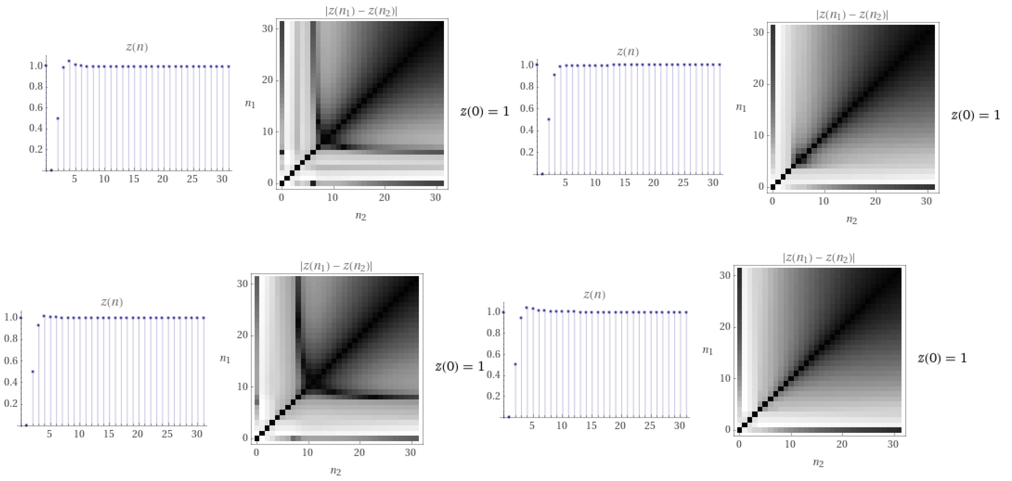
In this place, we iterate the solution of the integral Equation (19). We start with the iteration solution imposes (see Figure 4)
For we obtain the iteration solution
Moreover, for we obtain
Finally, we assume that then we have
Table 1 shows the number of iterations and the error, which calculated by
5. Conclusions
In our current work, we defined G-contraction and G-contraction of Darbo type and proved corresponding fixed-point theorems using . Furthermore, the fixed-point theorem proved in Section 2 is applied to demonstrate the existence of a solution of fractional-order integral equation. At the end, an example is given to validate the result. We indicate that the values of the fixed-point increase whenever the values of increase in Moreover, the set of fixed points imposed the periodicity and stability of the fractional integral Equation (20). All figures are presented with the help of Mathematica 11.2.
Author Contributions
Conceptualization, V.N. and D.G.; methodology, V.N. and D.G.; formal analysis, R.W.I.; investigation, V.N. and D.G. All authors have read and agreed to the published version of the manuscript.
Funding
This research received no external funding.
Institutional Review Board Statement
Not applicable.
Informed Consent Statement
Not applicable.
Data Availability Statement
No new data were created or analyzed in this study. Data sharing is not applicable to this article.
Acknowledgments
The authors would like to express their full thanks to the respected editorial office.
Conflicts of Interest
The authors declare no conflict of interest.
Abbreviations
| The closed ball centered at x with radius r | |
| The class of nonempty, bounded, closed and convex sets. | |
| Measure of noncompactness. | |
| Set of all real numbers. | |
| Set of all positive real numbers. | |
| Set of all positive integers. | |
| Closer of set . | |
| The family of all bounded subsets of the space E | |
| The subfamily of consisting only relatively compact sets. | |
| The convex hull and closed convex hull of respectively. |
References
- Jleli, M.; Karapinar, E.; O’Regan, D.; Samet, B. Some generalizations of Darbos theorem and applications to fractional integral equations. Fixed Point Theory Appl. 2016, 2016, 11. [Google Scholar] [CrossRef] [Green Version]
- Mursaleen, M.; Rizvi, S.M.H.; Samet, B. Measures of Noncompactness and Their Applications. In Advances in Nonlinear Analysis via the Concept of Measure of Noncompactness; Banaś, J., Jleli, M., Mursaleen, M., Samet, B., Vetro, C., Eds.; Springer: Singapore, 2017. [Google Scholar]
- Kuratowski, K. Topology: Volume I; Elsevier: Amsterdam, The Netherlands, 2014; Volume 1. [Google Scholar]
- Darbo, G. Punti uniti in trasformazioni a codominio non compatto. Rend. del Semin. Mat. della Univ. di Padova 1955, 24, 84–92. [Google Scholar]
- Wardowski, D. Fixed points of a new type of contractive mappings in complete metric spaces. Fixed Point Theory Appl. 2012, 2012, 94. [Google Scholar] [CrossRef] [Green Version]
- Banas, J. On measures of noncompactness in banach spaces. Comment. Math. Univ. Carol. 1980, 21, 131–143. [Google Scholar]
- Banas, J.; Merentes, N.; Rzepka, B. Measures of noncompactness in the space of continuous and bounded functions defined on the real half-axis. In Advances in Nonlinear Analysis via the Concept of Measure of Noncompactness; Springer: Berlin/Heidelberg, Germany, 2017; pp. 1–58. [Google Scholar]
- Banas, J.; Zajac, T. Solvability of a functional integral equation of fractional order in the class of functions having limits at infinity. Nonlinear Anal. Theory Methods Appl. 2009, 71, 5491–5500. [Google Scholar] [CrossRef]
- Schauder, J. Derxpunktsatz in funktionalraumen. Stud. Math. 1930, 2, 171–180. [Google Scholar] [CrossRef] [Green Version]
- Vetro, C.; Vetro, F. The class of f-contraction mappings with a measure of noncompactness. In Advances in Nonlinear Analysis via the Concept of Measure of Noncompactness; Springer: Berlin/Heidelberg, Germany, 2017; pp. 297–331. [Google Scholar]
- Agarwala, R.P.; Samet, B. An existence result for a class of nonlinear integral equations of fractional orders. Nonlinear Anal. Model. Control 2016, 21, 716–729. [Google Scholar] [CrossRef]
- Aghajani, A.; Pourhadi, E.; Trujillo, J.J. Application of measure of noncompactness to a Cauchy problem for fractional differential equations in Banach spaces. Fract. Calc. Appl. Anal. 2013, 16, 962–977. [Google Scholar] [CrossRef]
- Darwish, M.A. On monotonic solutions of a singular quadratic integral equation with supremum. Dynam. Syst. Appl. 2008, 17, 539–550. [Google Scholar]
- Darwish, M.A. On Erdelyi-kober fractional urysohn-Volterra quadratic integral equations. Appl. Math. Comput. 2016, 273, 562–569. [Google Scholar] [CrossRef]
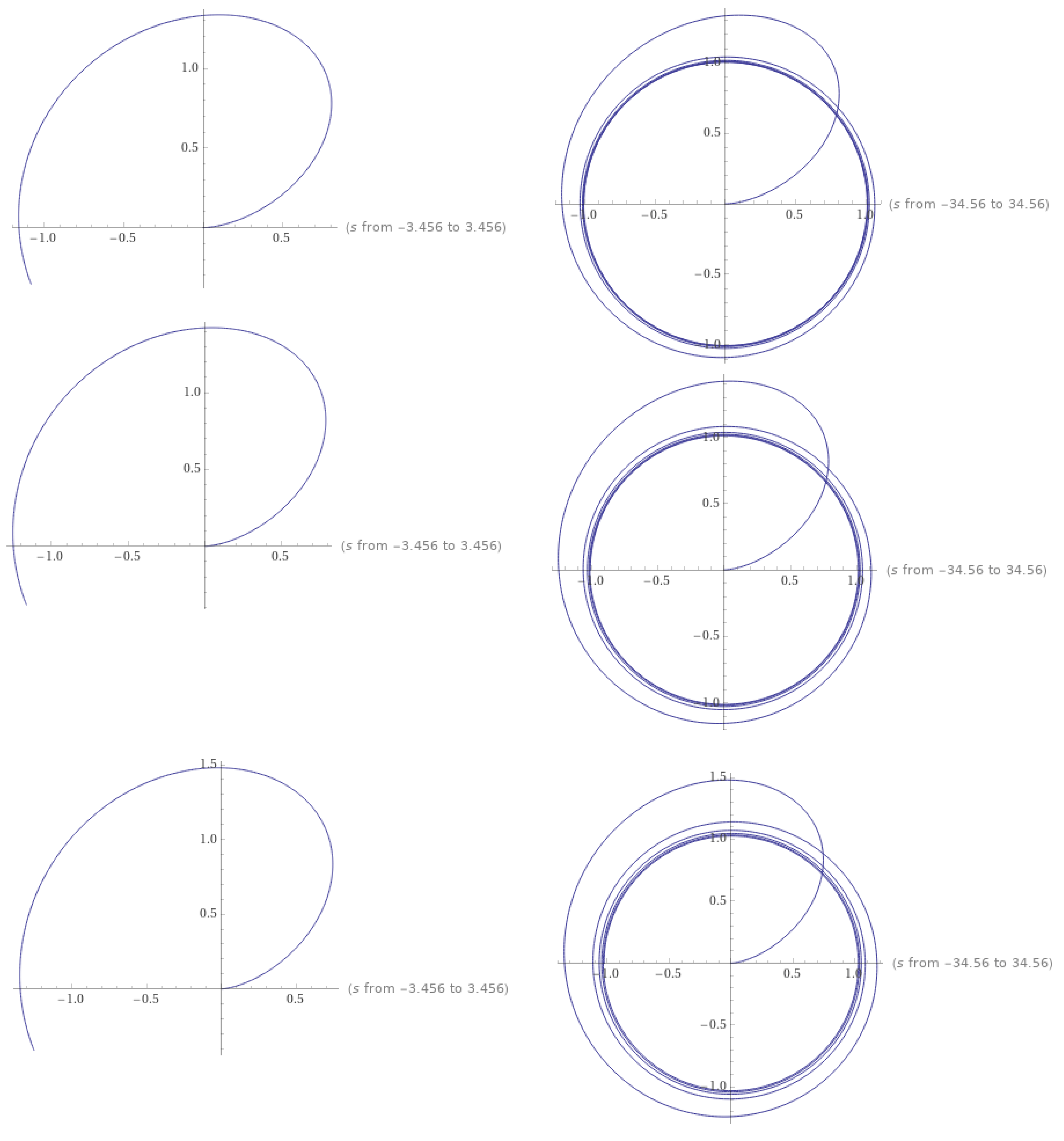
Figure 1.
The stable periodicity solution of based on the set of fixed points when respectively.

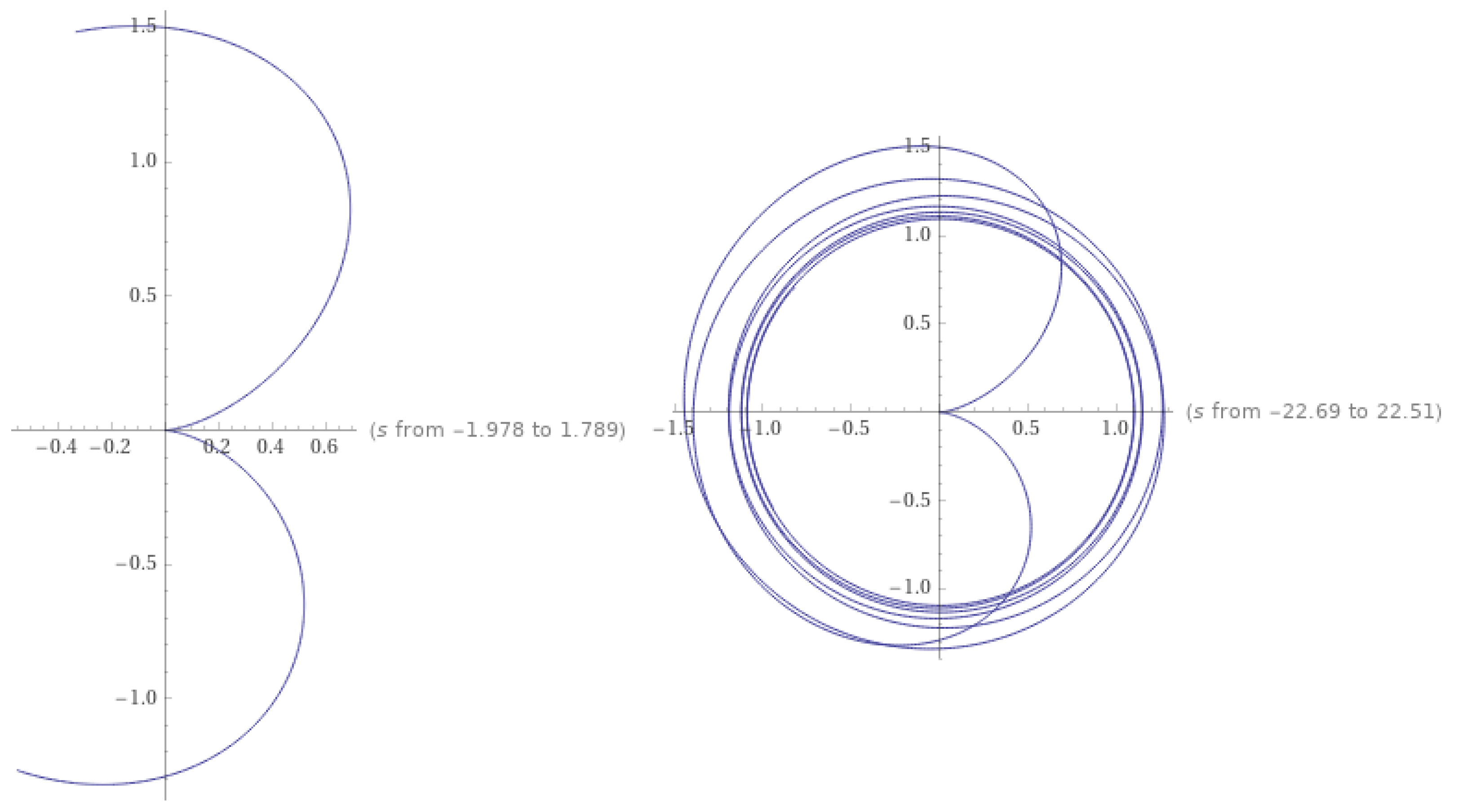
Figure 2.
The stable periodicity solution of based on the set of fixed points when and .

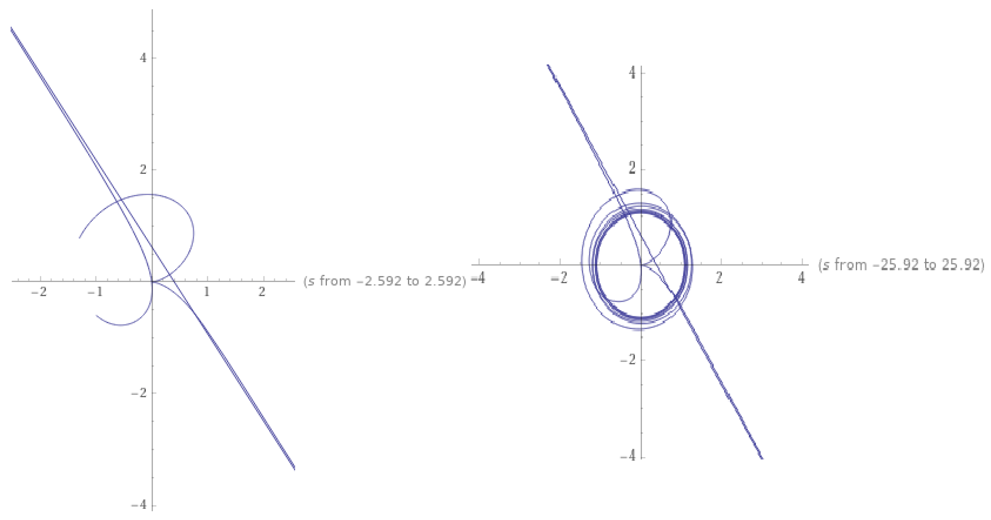
Figure 3.
The solution of based on the set of fixed points when and .

Figure 4.
The iteration solution of for respectively.


Table 1.
Iteration solution of Equation (19).
Table 1.
Iteration solution of Equation (19).
| n | 0 | 1 | 2 | 3 | 4 | Error = | |
|---|---|---|---|---|---|---|---|
| 1/4 | z(n) | 1 | 0 | 0.5 | 0.98829 | 1.04883 | 0.301 |
| 1/2 | z(n) | 1 | 0 | 0.5 | 0.908102 | 0.98557 | 0.41 |
| 3/4 | z(n) | 1 | 0 | 0.5 | 0.928555 | 1.01562 | 0.454 |
| 1 | z(n) | 1 | 0 | 0.5 | 0.941959 | 1.0437 | 0.464 |
Publisher’s Note: MDPI stays neutral with regard to jurisdictional claims in published maps and institutional affiliations. |
© 2021 by the authors. Licensee MDPI, Basel, Switzerland. This article is an open access article distributed under the terms and conditions of the Creative Commons Attribution (CC BY) license (https://creativecommons.org/licenses/by/4.0/).
Share and Cite
MDPI and ACS Style
Nikam, V.; Gopal, D.; Ibrahim, R.W. Solvability of a Parametric Fractional-Order Integral Equation Using Advance Darbo G-Contraction Theorem. Foundations 2021, 1, 286-303. https://0-doi-org.brum.beds.ac.uk/10.3390/foundations1020021
AMA Style
Nikam V, Gopal D, Ibrahim RW. Solvability of a Parametric Fractional-Order Integral Equation Using Advance Darbo G-Contraction Theorem. Foundations. 2021; 1(2):286-303. https://0-doi-org.brum.beds.ac.uk/10.3390/foundations1020021
Chicago/Turabian StyleNikam, Vishal, Dhananjay Gopal, and Rabha W. Ibrahim. 2021. "Solvability of a Parametric Fractional-Order Integral Equation Using Advance Darbo G-Contraction Theorem" Foundations 1, no. 2: 286-303. https://0-doi-org.brum.beds.ac.uk/10.3390/foundations1020021