Numerical Analysis of Viscoelastic Rotating Beam with Variable Fractional Order Model Using Shifted Bernstein–Legendre Polynomial Collocation Algorithm

Abstract

This paper applies a numerical method of polynomial function approximation to the numerical analysis of variable fractional order viscoelastic rotating beam. First, the governing equation of the viscoelastic rotating beam is established based on the variable fractional model of the viscoelastic material. Second, shifted Bernstein polynomials and Legendre polynomials are used as basis functions to approximate the governing equation and the original equation is converted to matrix product form. Based on the configuration method, the matrix equation is further transformed into algebraic equations and numerical solutions of the governing equation are obtained directly in the time domain. Finally, the efficiency of the proposed algorithm is proved by analyzing the numerical solutions of the displacement of rotating beam under different loads.

1. Introduction

Viscoelastic material is a material specially used as damping layer. Its main characteristics are related to temperature and frequency. Viscoelastic materials are also widely used in aerospace, construction, mechanical engineering and other fields. Polyurea is a kind of viscoelastic materials produced by the reaction of isocyanate and amino compound. Polyurea exhibits good aging resistance and thermal stability [1,2]. It can be used in various household chemicals. Polyethylene terephthalate polymer (PET) is composed by polyethylene terephthalate and polybutylene terephthalate. PET exhibits a smooth and shiny surface, good creep and fatigue resistance, and good friction resistance [3]. It is widely used in the electrical, electronic and automotive industries. The mechanical behaviors of these two viscoelastic materials are analyzed in this paper.

In recent years, the viscoelastic model has been widely used in the dynamic analysis of viscoelastic structures. Alotta et al. [4] proposed a non-local viscoelastic beam model and introduced a comprehensive numerical method to calculate the stochastic response of the non-local fractional beam model under Gaussian white noise. Numerical examples demonstrated the versatility of the non-local fractional model as well as computational advantages of the proposed solution procedure. These models are usually simulated by integer order or fractional order derivatives, such as Kelvin-Voigt model, Maxwell model, three-parameter solid model and Zener model and so on. Fractional model is now a well-established tool in engineering science, with very promising applications in materials modeling [5]. However, in most cases, the integer order or fractional order model cannot well describe the dynamic viscoelastic behavior [6]. In the dynamic analysis, the slight change of the parameters will cause the great change of the system. Under large strain conditions, variable fractional differential operators can better simulate viscoelastic constitutive relations than fractional differential operators [7]. How to characterize the memory property of systems is a challenging issue in the modeling and analysis of complex systems [8,9]. Sun et al. [10] made a comparative investigation of integer-order derivative, constant-order fractional derivative and two types of variable-order fractional derivatives in characterizing the memory property of systems. The advantages and potential applications of two-variable-order derivative definitions were highlighted through a comparative analysis of anomalous relaxation process. To accurately establish the viscoelastic constitutive relationship, a variable fractional order model is proposed. Meng et al. [11] studied the compression deformation of amorphous glassy polymers using variable fractional order model. The results demonstrated that the model has the advantages of high accuracy and few parameters. Wang and Chen [12] used a variable fraction model to analyze fluid dynamics in viscoelastic pipes. Therefore, the research in this article is based on the variable fractional order viscoelastic model.

With the development of viscoelastic models, many scholars apply viscoelastic models to dynamic analysis of beams. Lewandowski et al. [13] used a fractional Zener model to describe the non-linear vibration of a visco-elastic composite beam composed by the elastic and visco-elastic layers. The effect of harmonic force on non-linear vibration was investigated. Baum et al. [14] applied a four-parameter rheological model with fractional derivatives to describe the mechanical properties of the multi-layer composite beam. This innovative method was validated to determine the dynamic properties of the composite beam. Fernando et al. [15] used a five-parameter fractional derivative model to study the transient dynamics of a cantilever beam with different damping values under various loading conditions. However, the application of the viscoelastic variable fractional derivative model to the dynamic analysis of beams is still relatively rare. Therefore, in this paper, a numerical analysis is carried out on the variable fractional viscoelastic beam. A reliable method to accurately solve the problem of variable fractional equation is particularly critical. Chen et al. [16] used polynomials approximation methods to solve fractional and variable fractional differential equations. Numerical examples verified the accuracy and convergence of the method. Samaneh et al. [17] proposed an innovative algorithm to solve the variable-order fractional equations in the optimal control problems. The effectiveness of this method was verified according to the comparison with several common optimization methods. Hassani et al. [18] proposed an optimization method based on the Caputo type definition and a set of basic polynomial functions to solve the variable-order fractional non-linear Klein–Gordon equation. Paola et al. [19] proposed a novel numerical method to explore a fractional system whose non-linear viscoelastic behavior changes with time. This method was used to analyze the stress and strain response of the variable fractional order system. These studies confirm that the polynomial functions can be successfully used to solve the governing equations with variable fractional order.

Bernstein and Legendre polynomials are widely used as basic functions in numerical algorithms to solve fractional differential equations. Bernstein polynomials exhibit excellent stability and approximation. Rostamy et al. [20] employed Bernstein operational matrices to solve multi-order fractional differential equations. Maleknejad et al. [21] used Bernstein operational matrices to obtain the numerical solution of non-linear Volterra–Fredholm– Hammerstein integral equations. Legendre polynomials are orthogonal, and their weight function is uncomplicated compared to the other orthogonal polynomials, such as Chebyshev polynomial [22], Bernoulli polynomial [23] and so on. In this paper, an algorithm based on the Bernstein and Legendre polynomials is proposed to combine the advantages of these two polynomials. The displacement function of the beam is approximated by a series of basic functions based on the shifted Bernstein and Legendre polynomials. The derivative of the displacement function is represented by the product of the differential operator matrix. The algorithm is confirmed to be suitable and accurate for solving the governing equations with the variable fractional order models. The polynomial numerical algorithm method can be used to approximate the unknown function on the extended interval, which makes it easier to solve the fractional differential equations with different physical mechanisms governing and historical background [24,25].

The objective of this paper is to provide an efficient numerical method for the numerical analysis of variable fractional viscoelastic rotating beams. The numerical algorithm can directly obtain the numerical solution of the equation in the time domain, which greatly simplifies the calculation steps. Thus, this algorithm can provide a theoretical basis for the mechanical analysis of viscoelastic rotating beams. This paper is arranged as follows. In Section 2, the definition and properties of variable fractional differential operator are introduced. The governing equation of viscoelastic rotating beam is established based on the variable fractional model. In Section 3, the shifted Bernstein–Legendre polynomial collocation algorithm is described. In Section 4, the numerical solutions of the viscoelastic beam are analyzed under different loads. The research work is concluded in Section 5.

2. Mathematical Preliminaries

In this section, the mathematical definition and properties of variable fractional differential operator are introduced. The governing equation of the viscoelastic rotating beam is established by using a variable fractional order model.

2.1. Variable Fractional Differential Operators

Definition 1.

The Caputo definition of variable fractional differential operator ${(}^C{D}_t^{r\left(t\right)})$ of $r\left(t\right)$ order is given by [26,27,28]

$${}^C{D}_t^{r\left(t\right)}f\left(t\right)=\frac{1}{\Gamma (1-r(t\left)\right)}{\int }_{0+}^t{(t-\tau )}^{-r\left(t\right)}{f}^{\prime }\left(\tau \right)d\tau$$

(1)

where $0<r\left(t\right)\le 1$, $f\left(t\right)$ is continuous over interval $(0,+\infty )$ and is integrable over any subinterval of $[0,+\infty )$, $\Gamma (·)$ is Gamma function and it is defined by $\Gamma \left(z\right)={\int }_0^{\infty }{e}^{-t}{t}^{z-1}dt$.

According to the definition of Caputo variable fractional derivative, the following formula is obtained by [29]

$${}^C{D}_t^{r\left(t\right)}\left(x^m{t}^n\right)=\left\{\begin{array}{c}\frac{\Gamma (n+1)}{\Gamma (n+1-r(t\left)\right)}{t}^{n-r\left(t\right)}{x}^m,n=1,2\cdots \\ 0,n=0\end{array}\right.$$

(2)

When $x^m=1$ in Equation (2), it can be obtained as follows

$${}^C{D}_t^{r\left(t\right)}\left(t^n\right)=\left\{\begin{array}{c}\frac{\Gamma (n+1)}{\Gamma (n+1-r(t\left)\right)}{t}^{n-r\left(t\right)},n=1,2\cdots \\ 0,n=0\end{array}\right.$$

(3)

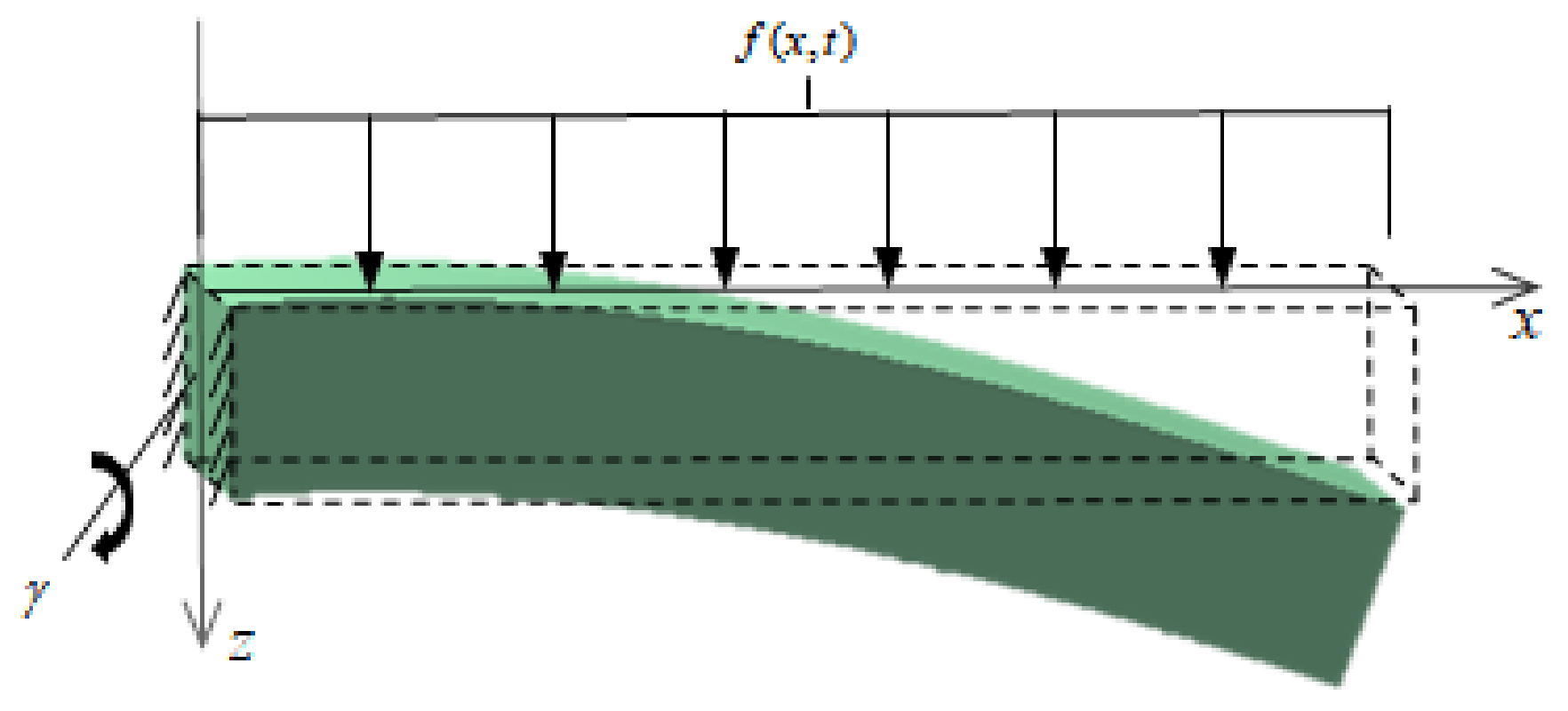
2.2. Establishment of Governing Equation with the Variable Fractional Viscoelastic Model

The force analysis of viscoelastic rotating beam is shown in Figure 1. A distributed load is applied in the vertical direction of the beam to produce displacement. x axis is the section center of the viscoelastic rotating beam, z is the axis perpendicular to the section, $f(x,t)$ is distributed load, $\omega (x,t)$ is the beam displacement, l is the length of the rotating beam, $\gamma$ is the speed.

The variable fractional order model of viscoelastic material is proposed as [7,30]

$$\sigma (x,t)=E{{\theta }^{r\left(t\right)}}^C{D}_t^{r\left(t\right)}\epsilon (x,t)$$

(4)

where $\sigma (x,t)$ is the normal stress on the cross-section S, E is Young’s modulus of the viscoelastic material, $\theta =\eta /E$, $\eta$ is the viscosity of the material, $\epsilon (x,t)$ is the strain and ${}^C{D}_t^{r\left(t\right)}$ is the Caputo variable fractional derivative of t.

The relationship between the strain and displacement of the rotating beam is given as

$$\epsilon (x,t)=-z\frac{{\partial }^2\omega (x,t)}{\partial x^2}$$

(5)

The relationship between bending moment and stress is given as

$$M(x,t)=\underset{S}{\int }z\sigma (x,t)dS$$

(6)

where $M(x,t)$ is the bending moment of the beam.

Substitute Equations (4) and (5) into Equation (6), the bending moment equation of the rotating beam is obtained

$$M(x,t)=E{\theta }^{r\left(t\right)}{I}^C{D}_t^{r\left(t\right)}\frac{{\partial }^2\omega (x,t)}{\partial x^2}$$

(7)

where $I=\underset{S}{\int }{z}^{2}dS$ is the moment of inertia.

The potential energy of the rotating beam is given as

$$U=\frac{1}{2}{\int }_0^{l}M(x,t)\frac{{\partial }^2\omega (x,t)}{\partial x^2}dx+\frac{1}{2}{\int }_0^l{T}_x\frac{{\partial }^2\omega (x,t)}{\partial x^2}dx$$

(8)

where $T_x=\rho S{\gamma }^{2}x$ is the centrifugal force during rotation. $\rho$ is the density of the viscoelastic beam.

The kinetic energy of the rotating beam is given as

$$T=\frac{1}{2}{\int }_0^l\rho S\frac{{\partial }^2\omega (x,t)}{\partial t^2}dx$$

(9)

From the Hamiltonian principle, the following equation can be obtained

$$\delta {\int }_{t_1}^{t_2}(T-U)dt+{\int }_{t_1}^{t_2}\delta \overline{W}dt=0$$

(10)

where the work done by the external load $\overline{W}=\frac{1}{2}{\int }_0^{l}f(x,t)\omega (x,t)dx$.

The governing equation of the viscoelastic rotating beam is obtained as

$$\rho S\frac{{\partial }^2\omega (x,t)}{\partial t^2}+E{\theta }^{r\left(t\right)}I{}^C{D}_t^{r\left(t\right)}\frac{{\partial }^4\omega (x,t)}{\partial x^4}-\rho S{\gamma }^{2}x\frac{{\partial }^2\omega (x,t)}{\partial x^2}=f(x,t)$$

(11)

The boundary conditions of the rotating beam are given by

$$\omega (0,t)=\frac{\partial \omega (0,t)}{\partial x}=0$$

(12)

$$\frac{{\partial }^2\omega (l,t)}{\partial x^2}=\frac{{\partial }^3\omega (l,t)}{\partial x^3}=0$$

(13)

The initial conditions are given by

$$\omega (x,0)=\frac{\partial \omega (x,0)}{\partial t}=0$$

(14)

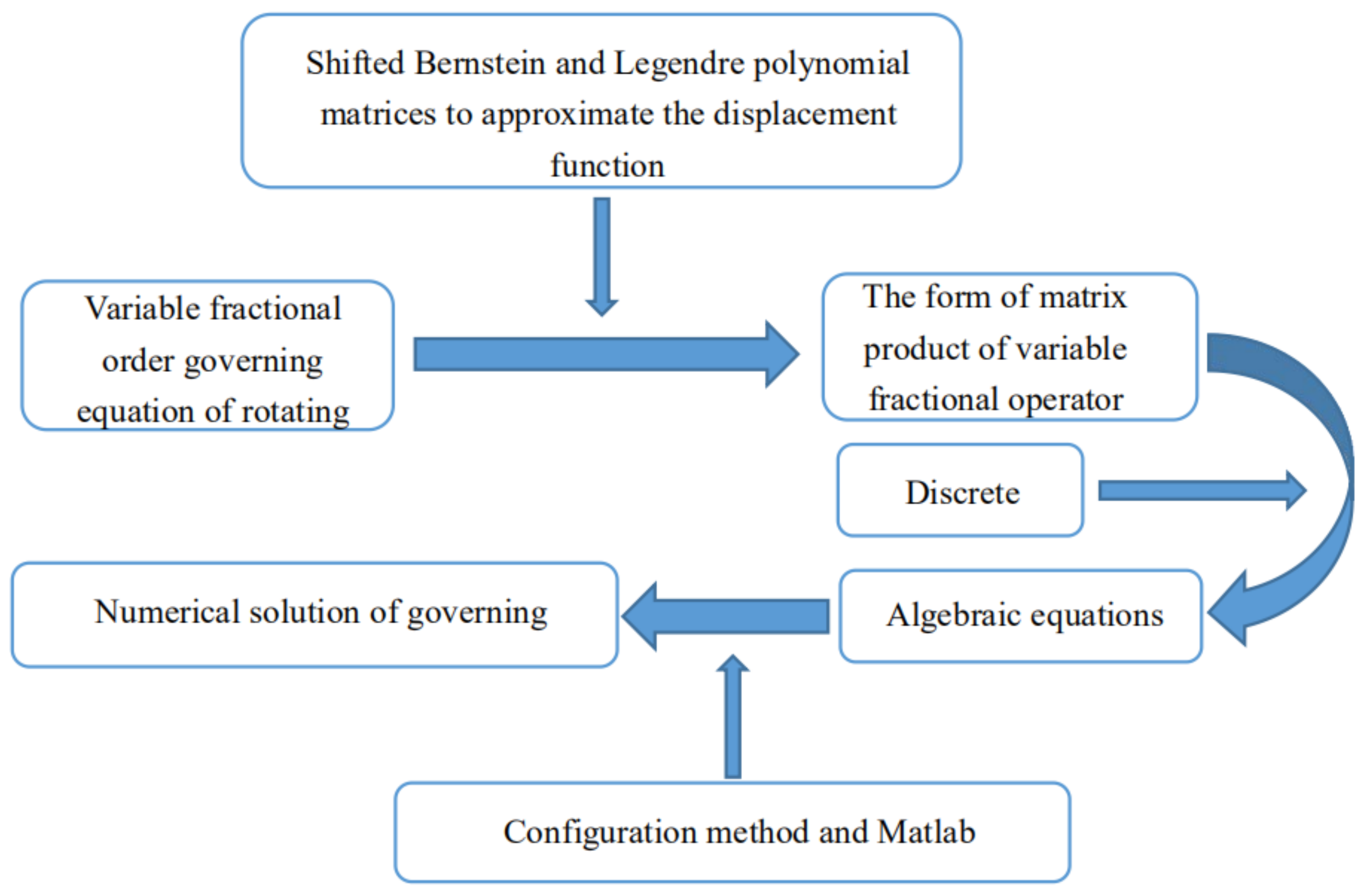
3. Shifted Bernstein–Legendre Polynomial Collocation Algorithm

In this section, a numerical algorithm is proposed to solve variable fractional equations based on Bernstein and Legendre polynomials. The schematic diagram of the algorithm is shown in Figure 2. Then, the specific process is shown in the following section. In the governing Equation (11) of the beam, the domain of the displacement $\omega (x,t)$ is $[0,R]\times [0,H]$. Theoretically, the values of R and H are close to positive infinity. However, in practical applications, the length and time of the beam are often accurate to a certain value. For reducing computations and improving efficiency in practical problems, the length x and the time t of the beam are selected as finite values. R and H are set to any positive number based on needs. Therefore, the base function of the displacement function is obtained by shifting the two types of polynomials on small interval.

In numerical algorithms, $\omega (x,t)$ is approximated by the shifted Bernstein polynomials in space direction and the shifted Legendre polynomials in time direction. The advantage of this algorithm is to convert the solution of variable fractional differential equation into the solution of algebraic equations. Therefore, the computation becomes very simple.

3.1. Shifted Bernstein–Legendre polynomial

Definition 2.

The Bernstein polynomial of degree n is defined by [31,32]

$$B_{n,i}\left(x\right)=\sum _{k=0}^{n-i}{(-1)}^k\left(\begin{array}{c}n\\ i\end{array}\right)\left(\begin{array}{c}n-i\\ k\end{array}\right)x^{i+k}$$

(15)

where $i=0,1,2,3.....n$, $x\in [0,1]$. To expand the range of x, the shifted Bernstein polynomial of degree n in $[0,R]$ is formulated as

$$\begin{array}{cc}\hfill {\overline{B}}_{n,i}\left(x\right)& =\left(\begin{array}{c}n\\ i\end{array}\right)\frac{x^i{(R-x)}^{n-i}}{R^n}\hfill \\ \hfill & =\sum _{k=0}^{n-i}{(-1)}^k\left(\begin{array}{c}n\\ i\end{array}\right)\left(\begin{array}{c}n-i\\ k\end{array}\right)\frac{1}{R^{i+k}}{x}^{i+k}\hfill \end{array}$$

(16)

Then, a sequence of shifted Bernstein polynomials matrix $\phi \left(x\right)$ is formulated as

$$\phi \left(x\right)={[{\overline{B}}_{n,0}\left(x\right),{\overline{B}}_{n,1}\left(x\right),...,{\overline{B}}_{n,n}\left(x\right)]}^T=A{T}_n\left(x\right)$$

(17)

where

$$A={\left[a_{i,j}\right]}_{i,j=0}^n,a_{i,j}=\left\{\begin{array}{c}\frac{{(-1)}^{j-i}\left(\begin{array}{c}n\\ i\end{array}\right)\left(\begin{array}{c}n-i\\ j-i\end{array}\right)}{R^j},j\le i\\ 0,j>i\end{array}\right.$$

(18)

$$T_n\left(x\right)={[1,x,\cdots x^n]}^T$$

(19)

A is the coefficient matrix of shifted Bernstein polynomials. A is invertible, so $T_n\left(x\right)$ is obtained as

$$T_n\left(x\right)=A^{-1}\phi \left(x\right)$$

(20)

Definition 3.

The Legendre polynomial of degree n is defined by [33,34]

$$L_{n,i}\left(t\right)=\sum _{i=0}^n{(-1)}^{n+i}\frac{\Gamma (n+i+1)}{\Gamma (n-i+1){(\Gamma (i+1\left)\right)}^2}{t}^i$$

(21)

where $i=0,1,2,3.....n$, $t\in [0,1]$. To expand the range of t, the shifted Legendre polynomial of degree n in $[0,H]$ is formulated as

$${\overline{L}}_{n,i}\left(t\right)=\sum _{i=0}^n{(-1)}^{n+i}\frac{\Gamma (n+i+1)}{\Gamma (n-i+1){(\Gamma (i+1\left)\right)}^2}\left(\frac{1}{H}\right)t^i$$

(22)

Then, a sequence of shifted Legendre polynomials matrix $\psi \left(t\right)$ is formulated as

$$\psi \left(t\right)={[{\overline{L}}_{n,0}\left(t\right),{\overline{L}}_{n,1}\left(t\right),\cdots {\overline{L}}_{n,n}\left(t\right)]}^T=N{T}_n\left(t\right)$$

(23)

where

$$N={\left[{\Lambda }_{i,j}\right]}_{i,j=0}^n,{\Lambda }_{i,j}=\left\{\begin{array}{c}{(-1)}^{i+j}\frac{\Gamma (i+j+1)}{\Gamma (i-j+1){(\Gamma (j+1\left)\right)}^2{H}^j},j\le i\\ 0,j>i\end{array}\right.$$

(24)

$$T_n\left(t\right)={[1,t,\cdots t^n]}^T$$

(25)

Since N is reversible, it can be rewritten as

$$T_n\left(t\right)=N^{-1}\psi \left(t\right)$$

(26)

3.2. Function Approximation

A one-dimensional integrable function $\omega \left(x\right),x\in [0,R]$ can be approximated by shifted Bernstein polynomials by the following formula

$$\begin{array}{cc}\hfill \omega \left(x\right)& =\underset{n\to \infty }{lim}\sum _{i=0}^n{c}_i{\overline{B}}_{n,i}\left(x\right)\hfill \\ \hfill & \approx \sum _{i=0}^n{c}_i{\overline{B}}_{n,i}\left(x\right)\hfill \\ \hfill & =C^T\phi \left(x\right)\hfill \end{array}$$

(27)

where $C^T=[c_0,c_1.\cdots c_n]$.

The inner product of ${\phi }^T\left(x\right)$ on both sides of Equation (27) is calculated as follows

$$\begin{array}{cc}\hfill <\omega \left(x\right),{\phi }^T\left(x\right)>& =C^T<\phi \left(x\right),{\phi }^T\left(x\right)>\hfill \\ \hfill & =C^{T}Q\hfill \end{array}$$

(28)

where $Q=<\phi \left(x\right),{\phi }^T\left(x\right)>={\left[q_{i,j}\right]}_{i,j=o}^n,q_{i,j}={\int }_0^R{\overline{B}}_{n,i}\left(x\right){\overline{B}}_{n,j}\left(x\right)dx$ and so $C^T=<\omega \left(x\right)$, ${\phi }^T\left(x\right)>Q^{-1}$.

Similarly, a one-dimensional integrable function $\omega \left(t\right),t\in [0,H]$ can be approximated by shifted Legendre polynomials by the following formula

$$\begin{array}{cc}\hfill \omega \left(t\right)& =\underset{n\to \infty }{lim}\sum _{i=0}^n{k}_i{\overline{L}}_{n,i}\left(t\right)\hfill \\ \hfill & \approx \sum _{i=0}^n{k}_i{\overline{L}}_{n,i}\left(t\right)\hfill \\ \hfill & =K^T\psi \left(t\right)\hfill \end{array}$$

(29)

where $K^T=[k_0,k_1,\cdots k_n]$.

The inner product of ${\psi }^T\left(t\right)$ on both sides of Equation (29) is calculated as follows

$$\begin{array}{cc}\hfill <\omega \left(t\right),{\psi }^T\left(t\right)>& =K^T<\psi \left(t\right),{\psi }^T\left(t\right)>\hfill \\ \hfill & =K^{T}P\hfill \end{array}$$

(30)

where $P=<\psi \left(t\right),{\psi }^T\left(t\right)>={\left[p_{i,j}\right]}_{i,j=o}^n,p_{i,j}={\int }_0^H{\overline{L}}_{n,i}\left(t\right){\overline{L}}_{n,j}\left(t\right)dt$ and so $K^T=<\omega \left(t\right)$, ${\psi }^T\left(t\right)>P^{-1}$.

In this paper, two-variable continuous function $\omega (x,t)\in L^2([0,R]\times [0,H])$ can be approximated

$$\begin{array}{cc}\hfill \omega (x,t)& =\underset{n\to \infty }{lim}\sum _{j=0}^n(\sum _{i=0}^n{c}_i{\overline{B}}_{n,i}\left(x\right))k_j{\overline{L}}_{n,j}\left(t\right)\hfill \\ \hfill & \approx \sum _{j=0}^n(\sum _{i=0}^n{c}_i{\overline{B}}_{n,i}\left(x\right))k_j{\overline{L}}_{n,j}\left(t\right)\hfill \\ \hfill & =\sum _{j=0}^n\sum _{i=0}^n{\overline{B}}_{n,i}\left(x\right)c_i{k}_j{\overline{L}}_{n,j}\left(t\right)\hfill \\ \hfill & ={\phi }^T\left(x\right)W\psi \left(t\right)\hfill \end{array}$$

(31)

where $W={\left[w_{i,j}\right]}_{i,j=0}^n,w_{i,j}=c_i{k}_j$.

3.3. Integer-Order Differential Operator Matrix

$\phi \left(x\right)$ is the matrix of a series of shifted Bernstein polynomials related to x, the derivative of $\phi \left(x\right)$ with respect to x is

$$\frac{d\phi \left(x\right)}{dx}=G_x\phi \left(x\right)$$

(32)

Then

$$G_x\phi \left(x\right)=G_{x}A{T}_n\left(x\right)=A\frac{d{T}_n\left(x\right)}{dx}=AV{T}_n\left(x\right)=AV{A}^{-1}\phi \left(x\right)$$

(33)

where

$$V={\left[v_{i,j}\right]}_{i,j=0}^n,v_{i,j}=\left\{\begin{array}{c}i,i=j+1\\ 0,i\ne j+1\end{array}\right.$$

(34)

$G_x=AV{A}^{-1}$ is the first order differential operator matrix of shifted Bernstein polynomials.

The nth derivative of $\phi \left(x\right)$ with respect to x can be obtained

$$\frac{d^n\phi \left(x\right)}{d{x}^n}=G_{nx}\phi \left(x\right),n\in N_{+}$$

(35)

Then

$$G_{nx}\phi \left(x\right)=G_{nx}A{T}_n\left(x\right)=A\frac{d^n{T}_n\left(x\right)}{d{x}^n}=A{V}^n{T}_n\left(x\right)=A{V}^n{A}^{-1}\phi \left(x\right)$$

(36)

$G_{nx}=A{V}^n{A}^{-1}$ is the n order differential operator matrix of shifted Bernstein polynomials.

According to Equations (31) and (36), the following equation is be obtained

$$\frac{{\partial }^n\omega (x,t)}{\partial x^n}\approx \frac{{\partial }^n\left({\phi }^T\left(x\right)W\psi \left(t\right)\right)}{\partial x^n}={(\frac{{\partial }^n\phi \left(x\right)}{\partial x^n})}^{T}W\psi \left(t\right)={\phi }^T\left(x\right)\left(G_{nx}^T\right)W\psi \left(t\right)$$

(37)

Similarly, $\psi \left(t\right)$ is the matrix of a series of shifted Legendre polynomials related t, the derivative of $\psi \left(t\right)$ with respect to t is

$$\frac{d\psi \left(t\right)}{dt}={\Omega }_t\psi \left(t\right)$$

(38)

Then

$${\Omega }_t\psi \left(t\right)={\Omega }_{t}N{T}_n\left(t\right)=N\frac{d{T}_n\left(t\right)}{dt}=NV{T}_n\left(t\right)=NV{N}^{-1}\psi \left(t\right)$$

(39)

${\Omega }_t=NV{N}^{-1}$ is the first order differential operator matrix of shifted Legendre polynomials.

The nth derivative of $\psi \left(t\right)$ with respect to t can be obtained

$$\frac{d^n\psi \left(t\right)}{d{t}^n}={\Omega }_{nt}\psi \left(t\right),n\in N_{+}$$

(40)

Then

$${\Omega }_{nt}\psi \left(t\right)={\Omega }_{nt}N{T}_n\left(t\right)=N\frac{d^n{T}_n\left(t\right)}{d{t}^n}=N{V}^n{T}_n\left(t\right)=N{V}^n{N}^{-1}\psi \left(t\right)$$

(41)

${\Omega }_{nt}=N{V}^n{N}^{-1}$ is the n order differential operator matrix of shifted Legendre polynomials.

According to Equations (31) and (41), the following equation is obtained

$$\frac{{\partial }^n\omega (x,t)}{\partial t^n}\approx \frac{{\partial }^n\left({\phi }^T\left(x\right)W\psi \left(t\right)\right)}{\partial t^n}={\phi }^T\left(x\right)W(\frac{{\partial }^n\psi \left(t\right)}{\partial t^n})={\phi }^T\left(x\right)W{\Omega }_{nt}\psi \left(t\right)$$

(42)

3.4. Variable Fractional Differential Operator Matrix

The $r\left(t\right)$ order derivative of $\psi \left(t\right)$ with respect to t is formulated as

$$\frac{d^{r\left(t\right)}\psi \left(t\right)}{d{t}^{r\left(t\right)}}={\varphi }_{r\left(t\right)t}\psi \left(t\right)$$

(43)

Then

$${\varphi }_{r\left(t\right)t}\psi \left(t\right)={\varphi }_{r\left(t\right)t}N{T}_n\left(t\right)=N\frac{d^{r\left(t\right)}{T}_n\left(t\right)}{d{t}^{r\left(t\right)}}=NF{T}_n\left(t\right)=NF{N}^{-1}\psi \left(t\right)$$

(44)

where

$$F={\left[f_{i,j}\right]}_{i,j=0}^n,f_{i,j}=\left\{\begin{array}{c}\frac{\Gamma (i+1)}{\Gamma (i+1-r(t\left)\right)}{t}^{-r\left(t\right)},i=j\ne 0\\ 0,else\end{array}\right.$$

(45)

${\varphi }_{r\left(t\right)t}=NF{N}^{-1}$ is the variable differential operator matrix of shifted Legendre polynomials.

According to Equations (37) and (44), the following equation is obtained

$$\begin{array}{cc}\hfill {}^C{D}_t^{r\left(t\right)}\frac{{\partial }^n\omega (x,t)}{\partial x^n}& {\approx }^C{D}_t^{r\left(t\right)}\frac{{\partial }^n\left({\phi }^T\left(x\right)W\psi \left(t\right)\right)}{\partial x^n}\hfill \\ \hfill & ={\left(\frac{{\partial }^n\phi \left(x\right)}{\partial x^n}\right)}^{T}W\frac{d^{r\left(t\right)}\psi \left(t\right)}{dt}\hfill \\ \hfill & ={\phi }^T\left(x\right){\left(G_{nx}^T\right)}^{n}W{\varphi }_{r\left(t\right)t}\psi \left(t\right)\hfill \end{array}$$

(46)

Based on Equations (37), (42) and (46), the governing equation of the rotating beam is reconverted into a matrix product form

$$\rho S{\phi }^T\left(x\right)W{\Omega }_{2t}\psi \left(t\right)+E{\theta }^{r\left(t\right)}I{\phi }^T\left(x\right)\left(G_{4x}^T\right)W{\varphi }_{r\left(t\right)t}\psi \left(t\right)-\rho S{\gamma }^{2}x{\phi }^T\left(x\right)\left(G_{2x}^T\right)W\psi \left(t\right)=f(x,t)$$

(47)

The initial and boundary conditions of the beam are rewritten as

$${\phi }^T\left(0\right)W\psi \left(t\right)={\phi }^T\left(0\right)\left(G_x^T\right)W\psi \left(t\right)=0$$

(48)

$${\phi }^T\left(l\right)\left(G_{2x}^T\right)W\psi \left(t\right)={\phi }^T\left(l\right)\left(G_{3x}^T\right)W\psi \left(t\right)=0$$

(49)

$${\phi }^T\left(x\right)W\psi \left(0\right)={\phi }^T\left(x\right)W{\Omega }_t\psi \left(0\right)=0$$

(50)

Based on the collocation method, the reasonable match points $x_i=i\frac{R}{n},i=0,1,2,\cdots n$ and $t_j=j\frac{H}{n},j=0,1,2,\cdots ,n$ have been used to discretize the variable $(x,t)$ to $(x_i,t_j)$. Equation (47) is transformed into a set of algebraic equations. The coefficient $w_{i,j}$$(i=0,1,2,\cdots n;j=0,1,2,\cdots n)$ is determinate by using Matlab platform and least square method. The numerical solutions of the variable fractional governing equation can be obtained.

4. Numerical Results and Analysis

The numerical solution is theoretically obtained by the shifted Bernstein-Legendre polynomial collocation algorithm when the order n of polynomials increases towards infinity. However, to simplify the calculation process, n is taken as a small certain value 4. The materials used for the viscoelastic beam are polyurea and PET. The simulation parameters [7] of the material under the variable fractional order model are shown in

Table 1. The identified parameters of the variable-order fractional model of polyuria and PET.

Beam	$\mathit{\rho }$	$\mathit{\theta }$	E	$\mathit{r}\left(\mathit{t}\right)$
polyurea	$1060\mathrm{kg}/{\mathrm{m}}^3$	$0.0012\mathrm{s}$	$1.2\times {10}^7\mathrm{Pa}$	$-0.1t+1$
PET	$1380\mathrm{kg}/{\mathrm{m}}^3$	$0.35\mathrm{s}$	$3\times {10}^7\mathrm{Pa}$	$-0.1t+1$

.

The length of the rotating beam is $l=5$ m and the cross-section area is $S=0.01{\mathrm{m}}^2$. Moment of inertia is $I=\frac{{0.1}^4}{12}{\mathrm{m}}^4$. Speed is $\gamma =\frac{\pi }{2}$. These parameters of polyurea are substituted into Equation (11). The governing equations are solved by shifted Bernstein–Legendre polynomial collocation algorithm.

Three different types of load, including the uniform load, linear load and simple harmonic load are applied on the viscoelastic rotating beam in this study. Figure 3 shows the evolution of the displacement of the polyurea beam with the uniform load $f(x,t)=10$ N, the linear load $f(x,t)=2x$ and the harmonic load $f(x,t)=sin2t$. Obviously, the displacement of the polyurea beam increases with the loading time under any load. This is consistent with the conclusion of the literature [35]. The correctness of the numerical results is verified.

Figure 4 shows the displacements of the polyurea beam under different uniform loads, linear loads and simple harmonic loads when $t=0.5\mathrm{s}$. Under loads, the displacements of polyurea beams show an increasing trend with uniform load, linear load slope and harmonic load frequency. These numerical results are consistent with the conclusion of the literature [35]. Literature [35] used Chebyshev polynomial algorithm to calculate the lateral displacement of fractional rotating beam. Compared with the fractional order model, the variable fractional constitutive model can more accurately simulate the properties of viscoelastic materials. It is further verified that the algorithm proposed in this paper has the advantages of high calculation accuracy and wide application range.

The parameters of the PET material are substituted into Equation (11) and the displacement numerical solutions are calculated. Figure 5 shows the comparison of the numerical solutions of the displacement of the polyurea beam and the PET beam under different load conditions. Obviously, the displacement of the PET beam is smaller than that of the polyurea beam under any load when $t=0.5\mathrm{s}$. The smaller the displacement is, the greater the damping of the corresponding viscoelastic material and the bending resistance are. Therefore, the PET beams have better bending resistance than the polyurea beams. The obtained results indicate that the properties of the material are consistent with the actual material properties. The numerical solution obtained by the proposed algorithm has a good accuracy in this paper. Thus, this algorithm can provide a theoretical basis for the research, development and performance prediction of damping materials.

5. Conclusions

In this paper, an effective numerical algorithm for solving the constitutive equation of variable fractional order viscoelastic rotating beam was proposed based on shifted Bernstein–Legendre polynomial collocation algorithm in the time domain. The variable fractional order model is used to analyze the inherent laws of the dynamic performance of viscoelastic damping materials, which can provide a theoretical basis for the research, development and performance prediction of damping materials. The conclusion of this paper is as follows.

(1)

The governing equation of viscoelastic rotating beams is established by variable fractional constitutive model.

(2)

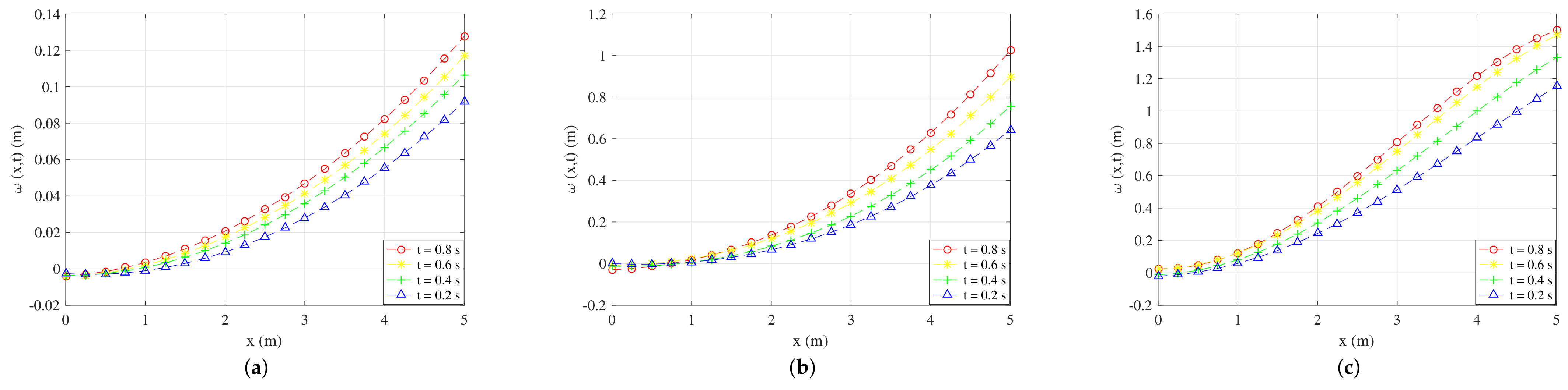
The displacement of the rotating beam increases with time under uniform load, linear load and simple harmonic load.

(3)

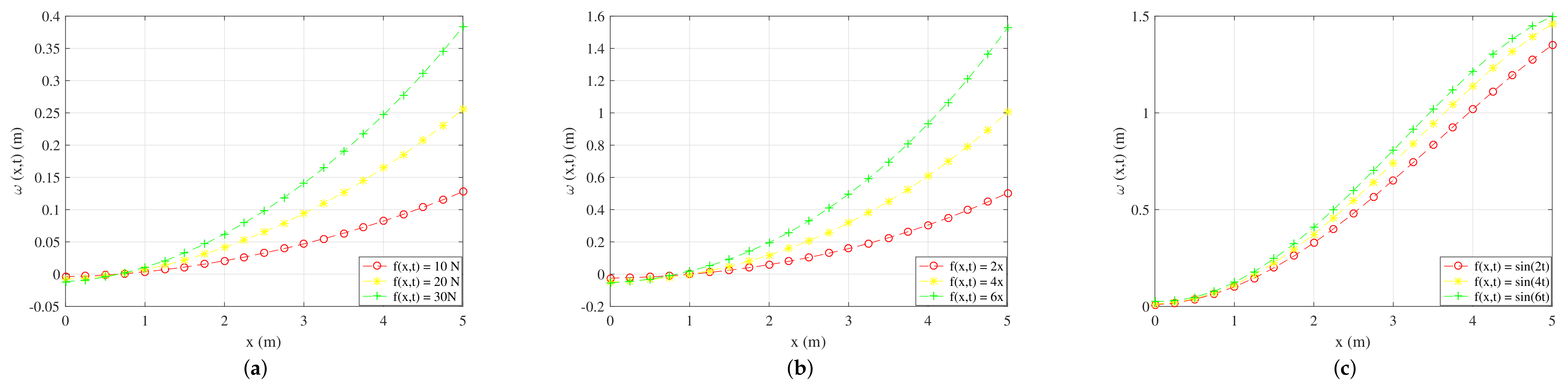
The displacements of rotating beams show an increasing trend with the increase of uniform load, linear load slope and simple harmonic load frequency.

(4)

The displacement of the PET beam is smaller than that of the polyurea beam, which theoretically verifies that PTE has better bending resistance than polyurea materials.

References

1. Roland, C.M.; Twigg, J.N.; Vu, Y.; Mott, P.H. High strain rate mechanical behavior of polyurea. Polymer 2007, 48, 574–578. [Google Scholar] [CrossRef]
2. Khajehsaeid, H.; Arghavani, J.; Naghdabadi, R.; Sohrabpour, S. A visco-hyperelastic constitutive model for rubber-like materials: A rate-dependent relaxation time scheme. Int. J. Eng. Sci. 2014, 79, 44–58. [Google Scholar] [CrossRef]
3. Boyce, M.C.; Socrate, S.; Llana, P.G. Constitutive model for the finite deformation stress–strain behavior of poly (ethylene terephthalate) above the glass transition. Polymer 2000, 41, 2183–2201. [Google Scholar] [CrossRef]
4. Alotta, G.; Paola, M.D.; Failla, G.; Pinnola, F.P. On the dynamics of non-local fractional viscoelastic beams under stochastic agencies. Compos. Part B Eng. 2018, 137, 102–110. [Google Scholar] [CrossRef]
5. Failla, G.; Zingales, M. Advanced materials modelling via fractional calculus: Challenges and perspectives. Philos. Trans. R. Soc. A 2020, 378, 20200050. [Google Scholar] [CrossRef] [PubMed]
6. Patnaik, S.; Hollkamp, J.P.; Semperlotti, F. Applications of variable-order fractional operators: A review. Proc. R. Soc. A 2019, 476, 20190498. [Google Scholar] [CrossRef] [Green Version]
7. Meng, R.F.; Yin, D.; Drapaca, C.S. A variable order fractional constitutive model of the viscoelastic behavior of polymers. Int. J. Non-Linear Mech. 2019, 113, 171–177. [Google Scholar] [CrossRef]
8. Lorenzo, C.F.; Hartley, T.T. Variable order and distributed order fractional operators. Nonlinear. Dynam. 2002, 29, 57–98. [Google Scholar] [CrossRef]
9. Coimbra, C.F.M. Mechanics with variable-order differential operators. Ann. Phys. 2003, 12, 692–703. [Google Scholar] [CrossRef]
10. Sun, H.G.; Chen, W.; Wei, H.; Chen, Y.Q. A comparative study of constant-order and variable-order fractional models in characterizing memory property of systems. Eur. Phys. J. Spec. Top. 2011, 193, 185–192. [Google Scholar] [CrossRef]
11. Meng, R.F.; Yin, D.; Drapaca, C.S. Variable-order fractional description of compression deformation of amorphous glassy polymers. Comput. Mech. 2019, 64, 163–171. [Google Scholar] [CrossRef]
12. Wang, Y.H.; Chen, Y.M. Dynamic analysis of the viscoelastic pipeline conveying fluid with an improved variable fractional order model based on shifted Legendre polynomials. Fractal Fract. 2019, 3, 52. [Google Scholar] [CrossRef] [Green Version]
13. Lewandowski, R.; Wielentejczyk, P. Nonlinear vibration of viscoelastic beams described using fractional order derivatives. J. Sound Vib. 2017, 399, 228–243. [Google Scholar] [CrossRef]
14. Lewandowski, R.; Baum, M. Dynamic characteristics of multilayered beams with viscoelastic layers described by the fractional Zener model. Arch. Appl. Mech. 2015, 85, 1793–1814. [Google Scholar] [CrossRef]
15. Fernando, C.; María, J.E. Finite element formulations for transient dynamic analysis in structural systems with viscoelastic treatments containing fractional derivative models. Int. J. Numer. Method Eng. 2007, 69, 2173–2195. [Google Scholar]
16. Wang, L.P.; Chen, Y.M.; Liu, D.Y.; Boutat, D. Numerical algorithm to solve generalized fractional pantograph equations with variable coefficients based on shifted Chebyshev polynomials. Int. J. Comput. Math. 2019, 96, 2487–2510. [Google Scholar] [CrossRef]
17. Samaneh, S.Z.; Hadi, J.S.; Amin, Y.F.; Stelios, B. King algorithm: A novel optimization approach based on variable-order fractional calculus with application in chaotic financial systems. Chaos Solitons Fractals 2020, 132, 109569. [Google Scholar]
18. Hassani, H.; Machadob, J.A.T.; Naraghirad, E. An efficient numerical technique for variable order time fractional nonlinear Klein-Gordon equation. Appl. Numer. Math. 2020, 154, 260–272. [Google Scholar] [CrossRef]
19. Paola, M.D.; Alotta, G.; Burlon, A.; Failla, G. A novel approach to nonlinear variable-order fractional viscoelasticity. Philos. Trans. R. Soc. A 2019, 378, 20190296. [Google Scholar] [CrossRef]
20. Rostamy, D.; Jafari, H.; Alipour, M.; Khalique, C.M. Computational method based on Bernstein operational matrices for multi-order fractional differential equations. Filomat 2014, 28, 591–601. [Google Scholar] [CrossRef] [Green Version]
21. Maleknejad, K.; Hashemizadeh, E.; Basirat, B. Computational method based on Bernstein operational matrices for nonlinear Volterra-Fredholm-Hammerstein integral equations. Commun. Nonlinear Sci. 2012, 17, 52–61. [Google Scholar] [CrossRef]
22. Huang, Y.X.; Zhao, Y.; Wang, T.S.; Tian, H. A new Chebyshev spectral approach for vibration of in-plane functionally graded Mindlin plates with variable thickness. Appl. Math. Model. 2019, 74, 21–42. [Google Scholar] [CrossRef]
23. Ren, Q.W.; Tian, H.J. Numerical solution of the static beam problem by Bernoulli collocation method. Appl. Math. Model. 2016, 40, 8886–8897. [Google Scholar] [CrossRef] [Green Version]
24. Cao, J.W.; Chen, Y.M.; Wang, Y.H.; Cheng, G.; Barrière, T. Shifted Legendre polynomials algorithm used for the dynamic analysis of PMMA viscoelastic beam with an improved fractional model. Chaos Solitons Fractals 2020, 141, 110342. [Google Scholar] [CrossRef]
25. Feng, Y.J.; Chen, Y.M.; Cheng, G.; Barrière, T. Numerical analysis of fractional-order variable section cantilever beams. ICIC Express Lett. 2010, 4, 5. [Google Scholar]
26. Malmir, I. A new fractional integration operational matrix of Chebyshev wavelets in fractional delay systems. Fractal Fract. 2019, 3, 46. [Google Scholar] [CrossRef] [Green Version]
27. Chen, Y.M.; Liu, L.Q.; Liu, D.Y.; Boutat, D. Numerical study of a class of variable order nonlinear fractional differential equation in terms of Bernstein polynomials. Ain Shams Eng. J. 2018, 9, 1235–1241. [Google Scholar] [CrossRef] [Green Version]
28. Samko, S.G. Fractional integration and differentiation of variable order. Anal. Math. 1995, 21, 213–236. [Google Scholar] [CrossRef]
29. Chen, Y.M.; Liu, L.Q.; Li, B.F.; Sun, Y.N. Numerical solution for the variable order linear cable equation with Bernstein polynomials. Appl. Math. Comput. 2014, 238, 329–341. [Google Scholar] [CrossRef]
30. Wang, Y.H.; Chen, Y.M. Shifted Legendre polynomials algorithm used for the dynamic analysis of viscoelastic pipes conveying fluid with variable fractional order model. Appl. Math. Model. 2020, 81, 159–176. [Google Scholar] [CrossRef]
31. Mirzaee, F.; Samadyar, N. Application of orthonormal Bernstein polynomials to construct a efficient scheme for solving fractional stochastic integro-differential equation. Optik 2017, 132, 262–273. [Google Scholar] [CrossRef]
32. Khataybeh, S.N.; Hashim, I.; Alshbool, M. Solving directly third-order ODEs using operational matrices of Bernstein polynomials method with applications to fluid flow equations. J. King. Saud. Univ. Sci. 2019, 31, 822–826. [Google Scholar] [CrossRef]
33. Xu, Y.; Zhang, Y.M.; Zhao, J.J. Error analysis of the Legendre-Gauss collocation methods for the nonlinear distributed-order fractional differential equation. Appl. Numer. Math. 2019, 142, 122–138. [Google Scholar] [CrossRef]
34. Sakar, M.J.; Saldır, O. A new reproducing kernel approach for nonlinear fractional three-point boundary value problems. Fractal Fract. 2020, 4, 53. [Google Scholar] [CrossRef]
35. Wang, L.; Chen, Y.M. Shifted-Chebyshev-polynomial-based numerical algorithm for fractional order polymer visco-elastic rotating beam. Chaos Solitons Fractals 2020, 132, 109585. [Google Scholar] [CrossRef]
Figure 1. Schematic of the rotating beam.
Fractalfract 05 00008 g001
Figure 2. Schematic diagram of the shifted Bernstein–Legendre polynomial collocation algorithm.
Fractalfract 05 00008 g002
Figure 3. Numerical solutions of the displacement of polyurea beam at different moments and different loads: (a) f ( x , t ) = 10 N, (b) f ( x , t ) = 2 x , (c) f ( x , t ) = s i n 2 t .
Fractalfract 05 00008 g003
Figure 4. Numerical solutions of the displacement of polyurea beam at the same time and under different loads: (a) Uniform loads (b) Linear loads (c) Simple harmonic loads.
Fractalfract 05 00008 g004
Figure 5. Comparison of numerical solutions for displacements of the polyurea beam and PET beam under different loads: (a) f ( x , t ) = 10 N, (b) f ( x , t ) = 2 x , (c) f ( x , t ) = s i n 2 t .
Fractalfract 05 00008 g005