
Novel Fractional Swarming with Key Term Separation for Input Nonlinear Control Autoregressive Systems

 , , and
Abstract
:1. Introduction
1.1. Literature Review
1.2. Contribution
- A key term separation technique-based fractional-order particle swarm optimization, KTST-FOPSO, is presented for parameter estimation of input nonlinear control autoregressive, IN-CAR systems.
- The KTST-FOPSO is developed through the synergy of PSO swarming intelligence with concepts of fractional calculus operators and the principle of the key term separation technique.
- The KTST-FOPSO is more efficient than the conventional FO-PSO in the sense that it identifies the IN-CAR system without estimating the extra parameters involved in the over-parameterization approach.
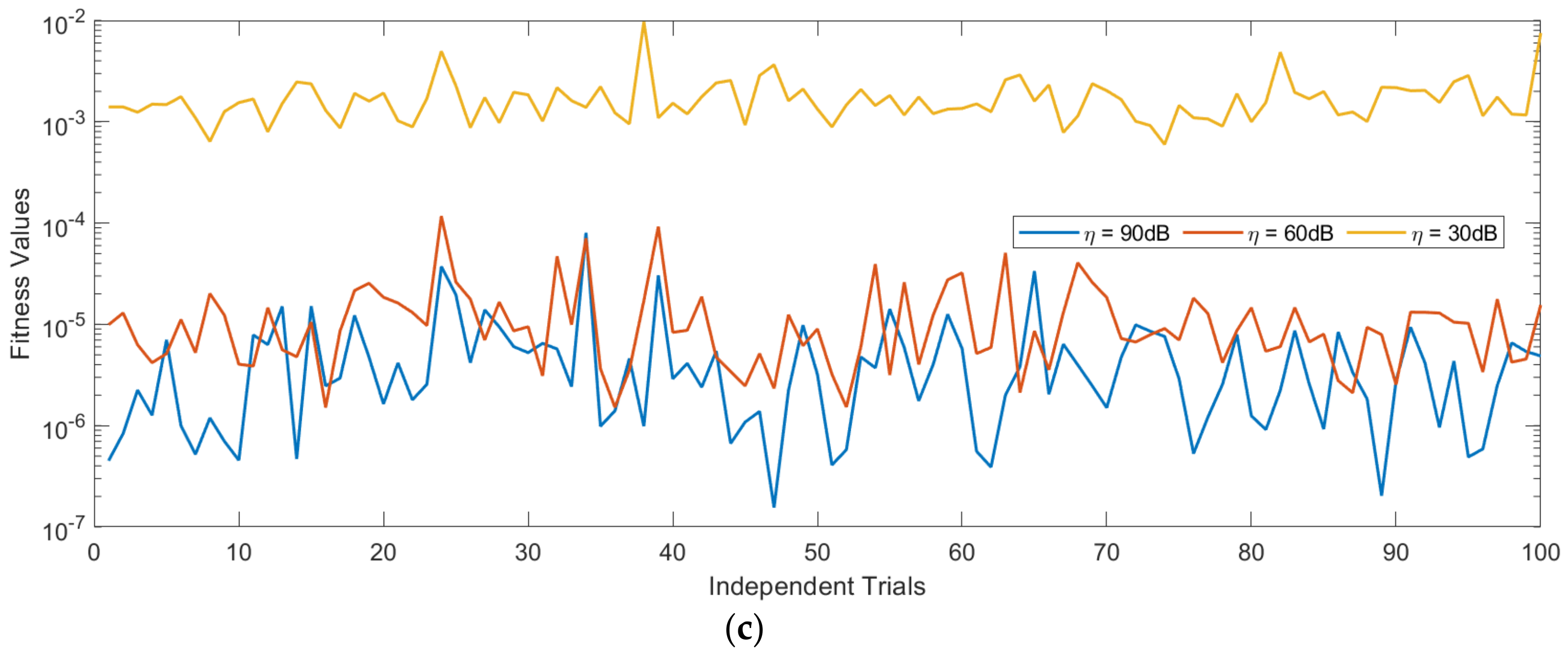
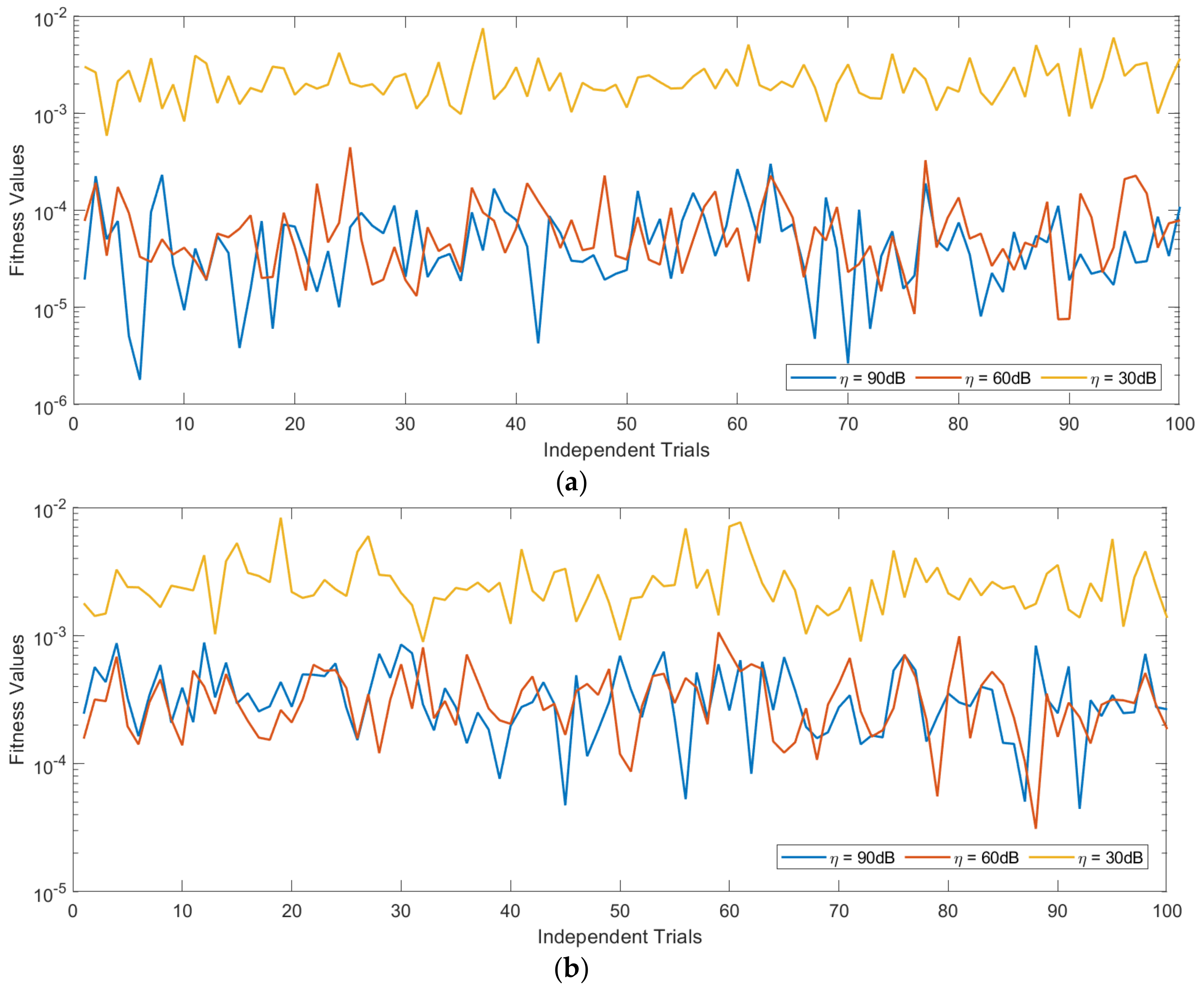
- The accuracy, robustness, convergence, reliability, and stability of the KTST-FOPSO scheme are verified through the results of statistical indices for different fractional orders and noise levels.
1.3. Paper Outline
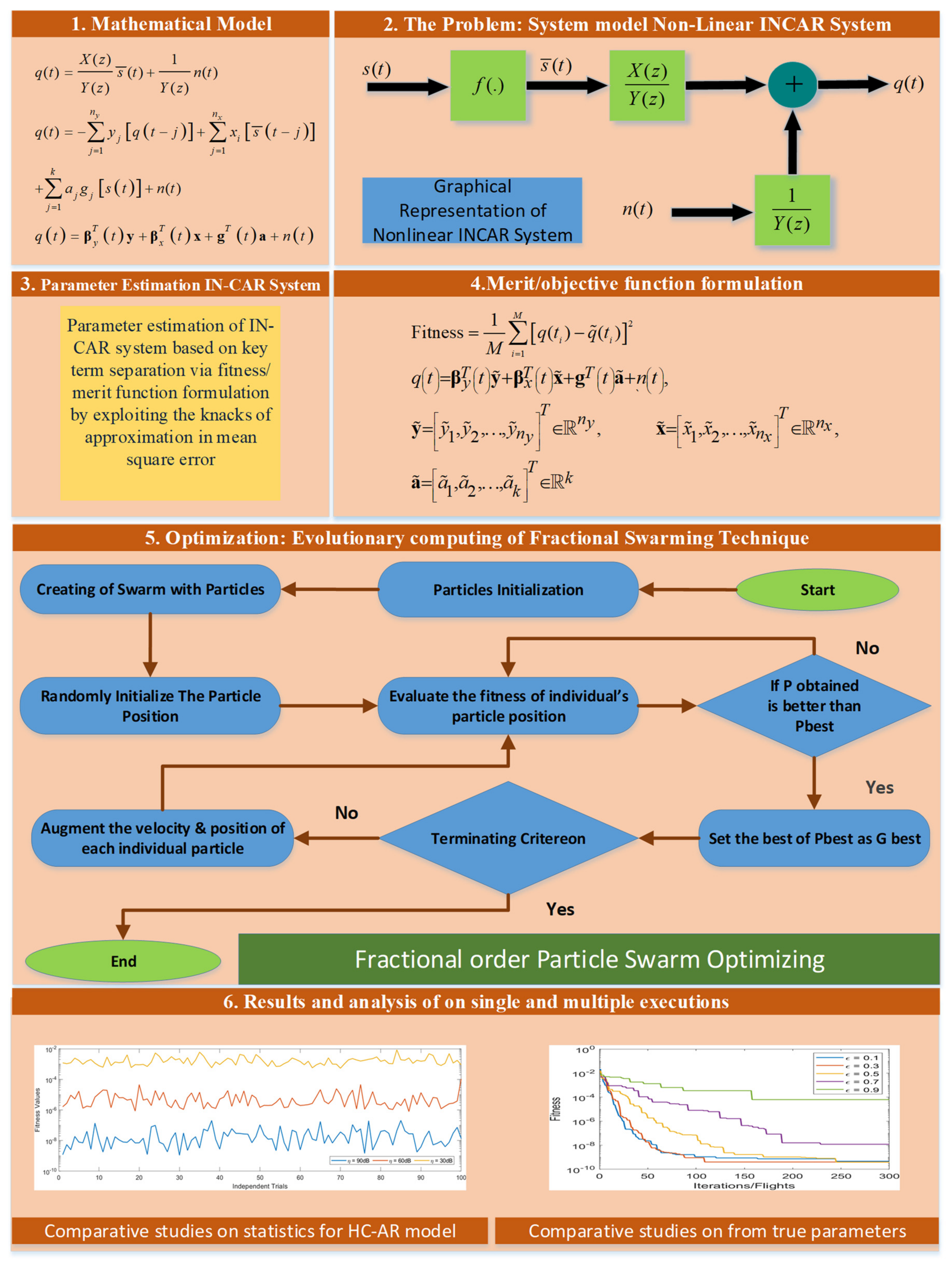
2. IN-CAR Identification Model
3. Proposed Methodology KTST-FOPSO
3.1. Formulation of the Objective Function
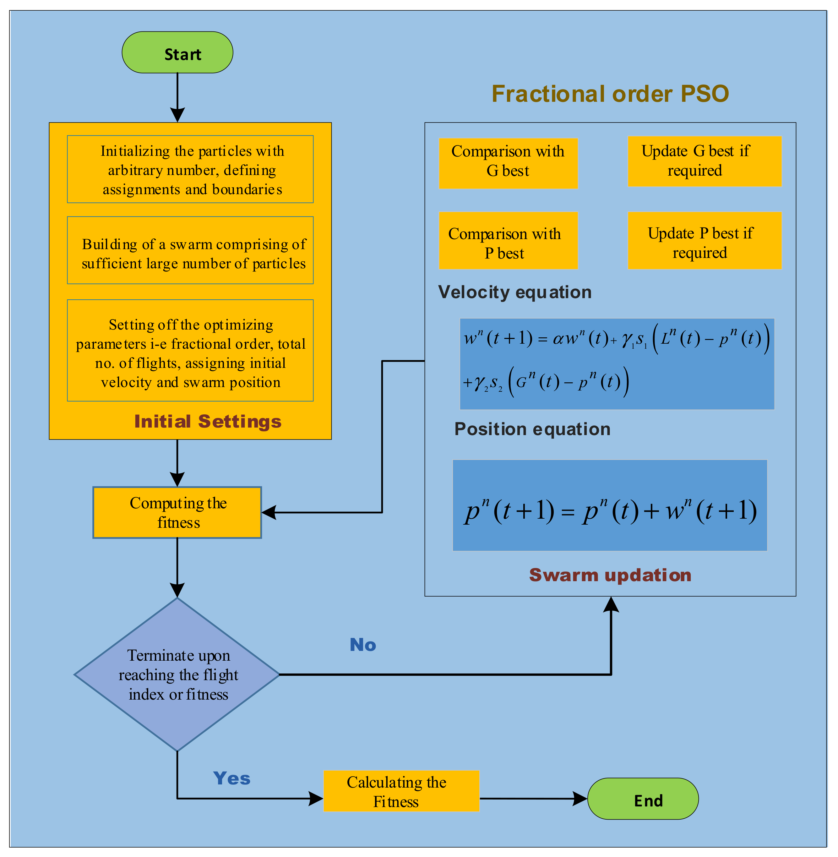
3.2. Fractional Order Swarm Optimization
| Algorithm 1: Pseudocode of the KTST-FOPSO for parameter estimation of the IN-CAR system | ||
| Inputs: | Create particle z with elements equal to the unknown parameter of the IN-CAR system | |
| and generate a swarm. | ||
| Swarm position, | ||
| for m number of particles z in Z. Similarly, the corresponding velocity w is generated. | ||
| Output: | The particle z of the KTST-FOPSO with the best fitness defined in (14) | |
| Start KTST-FOPSO | ||
| Step 1: | Initialization: pseudo-real number with are Randomly generated to form initialize swarm Z with m number of particles z. | |
| Initialize the associated velocities w to each particle | ||
| Set the minimum and maximum values of the velocity | ||
| Set particle and swarm size, flights number | ||
| Set the value of inertia weight and fractional order | ||
| Set the values for cognitive and social acceleration coefficients | ||
| Step 2: | Fitness Calculation: Calculate the fitness of each particle using (14). | |
| Step 3: | Termination: Terminate the KTST-FOPSO execution processing in case of the following:
| |
| If any of the above termination criteria are achieved, go to Step 5. | ||
| Step 4: | Update Mechanism: Update the swarm population by updating the position and velocity of the KTST-FOPSO defined in (20) and (27), respectively, and go to Step 2. | |
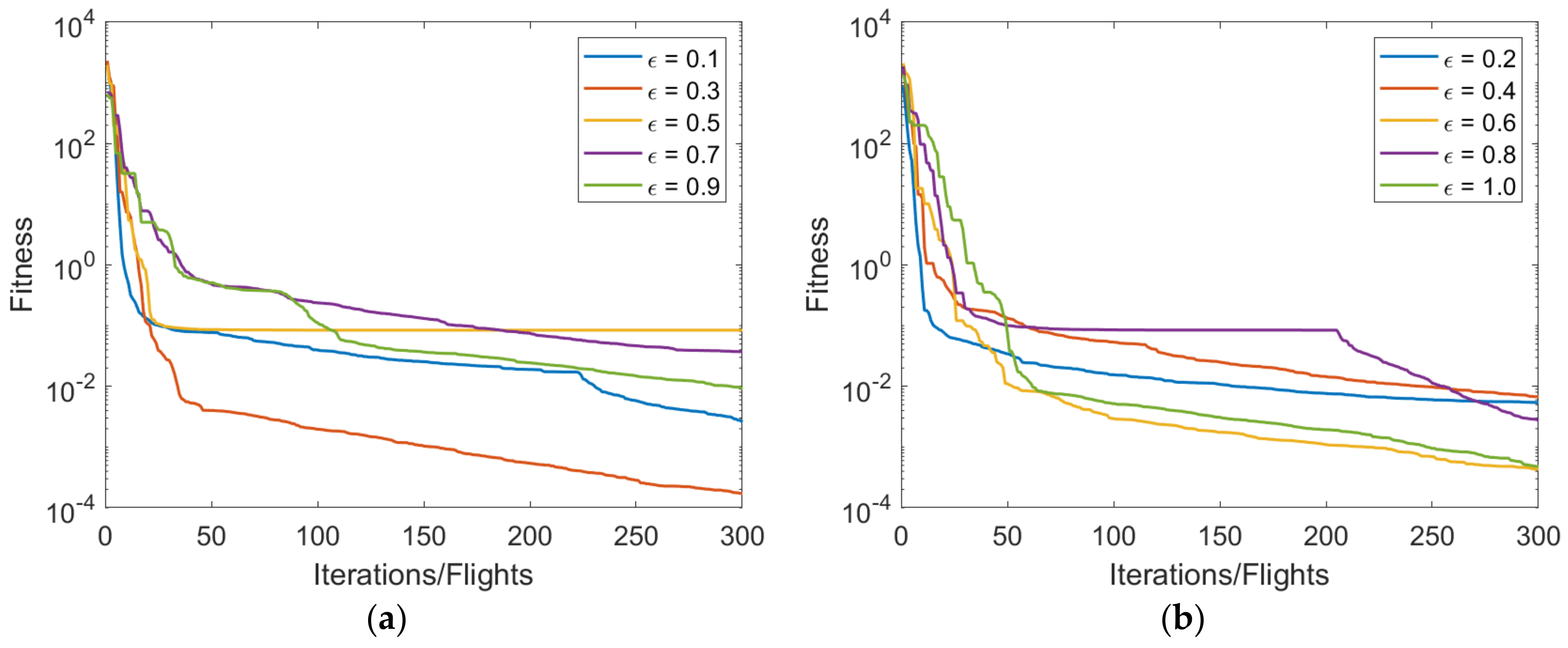
| Step 5: | Fractional Order Analysis: Get the results for different fractional order values through repeating Steps 1 to 4 by considering varying fractional orders in the KTST-FOPSO. | |
| Step 6: | Storage: Keeping the value for global best particle with corresponding fitness. | |
| Step 7: | Robustness Analysis: Repeat Steps 1–6 by considering different noise levels in the IN-CAR systems. | |
| Step 8: | Statistical Analysis: Obtain a dataset by repeated execution of the KTST-FOPSO scheme for parameter estimation of IN-CAR systems through multiple independent trials for reliable and accurate inferences. | |
| End FOPSO | ||
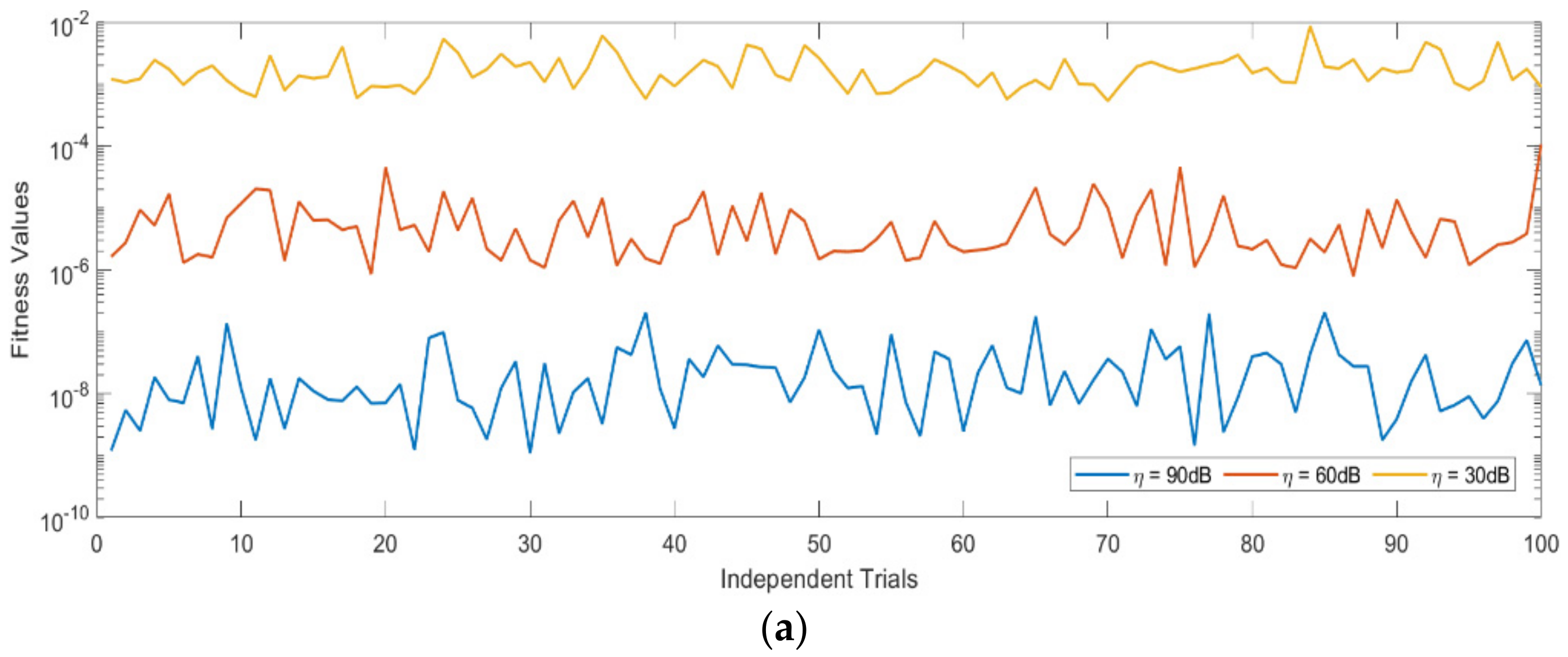
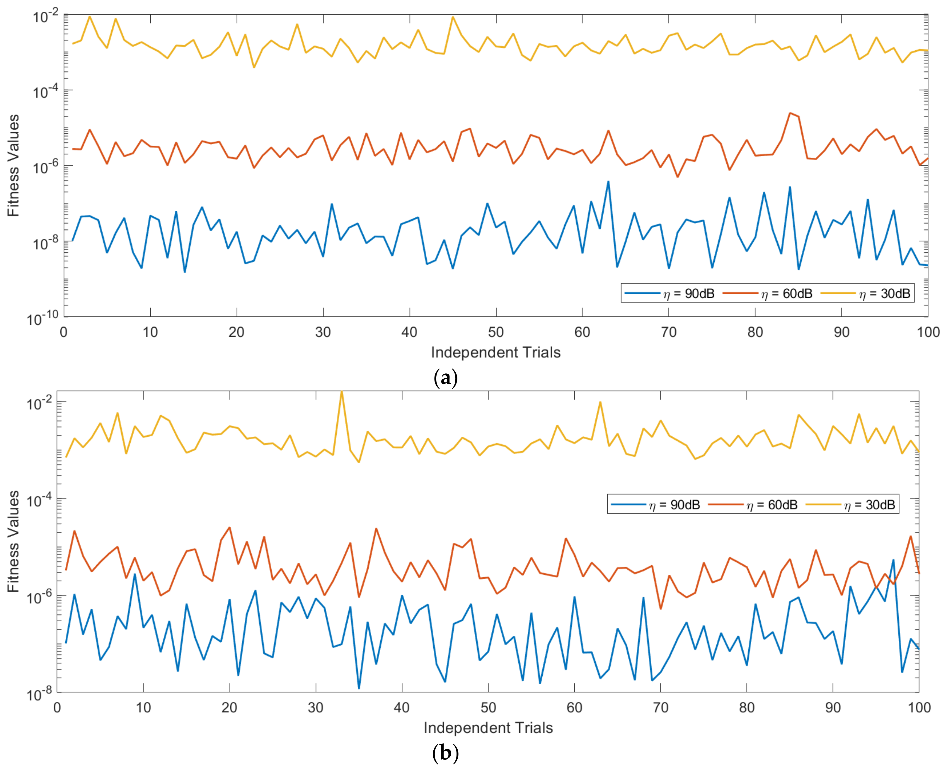
4. Results with Discussion
4.1. Example 1: Numerical Experimentation
4.2. Example 2: Electrical Stimulated Muscle Model
5. Conclusions
- A key term separation technique-based fractional order particle swarm optimization, KTST-FOPSO, is presented as an effective solution for the nonlinear system identification problem.
- The accuracy and robustness of the KTST-FOPSO are established through effective parameter estimation of input nonlinear control autoregressive, IN-CAR, systems for different fractional order and noise scenarios with generally a decreasing trend in estimation accuracy as fractional order increases from 0.1 to 1.
- The KTST-FOPSO is more efficient than the conventional FO-PSO in the sense that it avoids estimation of the redundant parameters and identifies only the actual parameters of the IN-CAR system.
- The reliability and stability of the KTST-FOPSO scheme are endorsed through results of statistical indices obtained after conducting sufficient large executions of the proposed scheme for numerical as well as practical examples of the IN-CAR system.
Supplementary Materials
Author Contributions
Funding
Data Availability Statement
Acknowledgments
Conflicts of Interest
References
- Sun, H.; Zhang, Y.; Baleanu, D.; Chen, W.; Chen, Y. A new collection of real world applications of fractional calculus in science and engineering. Commun. Nonlinear Sci. Numer. Simul. 2018, 64, 213–231. [Google Scholar] [CrossRef]
- Atangana, A.; Gómez-Aguilar, J.F. Decolonisation of fractional calculus rules: Breaking commutativity and associativity to capture more natural phenomena. Eur. Phys. J. Plus 2018, 133, 166. [Google Scholar] [CrossRef]
- Singh, J.; Kumar, D.; Hammouch, Z.; Atangana, A. A fractional epidemiological model for computer viruses pertaining to a new fractional derivative. Appl. Math. Comput. 2018, 316, 504–515. [Google Scholar] [CrossRef]
- Atangana, A.; Nieto, J.J. Numerical solution for the model of RLC circuit via the fractional derivative without singular kernel. Adv. Mech. Eng. 2015, 7. [Google Scholar] [CrossRef]
- Atangana, A.; Alkahtani, B.S.T. Extension of the resistance, inductance, capacitance electrical circuit to fractional derivative without singular kernel. Adv. Mech. Eng. 2015, 7. [Google Scholar] [CrossRef]
- Baleanu, D.; Diethelm, K.; Scalas, E.; Trujillo, J.J. Fractional Calculus: Models and Numerical Methods; World Scientific: Singapore, 2012; Volume 3. [Google Scholar]
- Giusti, A.; Colombaro, I.; Garra, R.; Garrappa, R.; Polito, F.; Popolizio, M.; Mainardi, F. A practical guide to Prabhakar fractional calculus. Fract. Calc. Appl. Anal. 2020, 23, 9–54. [Google Scholar] [CrossRef] [Green Version]
- Tarasov, V.E. On history of mathematical economics: Application of fractional calculus. Mathematics 2019, 3, 6559. [Google Scholar] [CrossRef] [Green Version]
- Diethelm, K.; Kiryakova, V.; Luchko, Y.; Machado, J.A.T.; Tarasov, V.E. Trends, directions for further research, and some open problems of fractional calculus. Nonlinear Dyn. 2022, 107, 3245–3270. [Google Scholar] [CrossRef]
- Khan, Z.A.; Zubair, S.; Alquhayz, H.; Azeem, M.; Ditta, A. Design of momentum fractional stochastic gradient descent for recommender systems. IEEE Access 2019, 7, 179575–179590. [Google Scholar] [CrossRef]
- Khokhar, N.M.; Majeed, M.N.; Shah, S.M. Diffusion Based Channel Gains Estimation in WSN Using Fractional Order Strategies. Comput. Mater. Contin. 2022, 70, 2209–2224. [Google Scholar]
- Xue, H. Fractional-order gradient descent with momentum for RBF neural network-based AIS trajectory restoration. Soft Comput. 2021, 25, 869–882. [Google Scholar] [CrossRef]
- Subudhi, U.; Sahoo, H.K. Adaptive estimation of sequence components for three-phase unbalanced system using fractional LMS/F algorithm. Electr. Eng. 2022, 104, 1757–1768. [Google Scholar] [CrossRef]
- Wang, X.; Fečkan, M.; Wang, J. Forecasting Economic Growth of the Group of Seven via Fractional-Order Gradient Descent Approach. Axioms 2021, 10, 257. [Google Scholar] [CrossRef]
- Yongjiang, L.U.O.; Luhao, B.I.; Dong, Z.H.A.O. Adaptive digital self-interference cancellation based on fractional order LMS in LFMCW radar. J. Syst. Eng. Electron. 2021, 32, 573–583. [Google Scholar] [CrossRef]
- Liu, J.; Zhai, R.; Liu, Y.; Li, W.; Wang, B.; Huang, L. A quasi fractional order gradient descent method with adaptive stepsize and its application in system identification. Appl. Math. Comput. 2021, 393, 125797. [Google Scholar] [CrossRef]
- Xu, T.; Chen, J.; Pu, Y.; Guo, L. Fractional-Based Stochastic Gradient Algorithms for Time-Delayed ARX Models. Circuits Syst. Signal Process. 2022, 41, 1895–1912. [Google Scholar] [CrossRef]
- Xu, C.; Mao, Y. Auxiliary Model-Based Multi-Innovation Fractional Stochastic Gradient Algorithm for Hammerstein Output-Error Systems. Machines 2021, 9, 247. [Google Scholar] [CrossRef]
- Nels, S.N.; Singh, J.A.P. Hierarchical Fractional Quantized Kernel Least mean Square Filter in Wireless Sensor Network for Data Aggregation. Wirel. Pers. Commun. 2021, 120, 1171–1192. [Google Scholar] [CrossRef]
- Kan, T.; Gao, Z.; Yang, C.; Jian, J. Convolutional neural networks based on fractional-order momentum for parameter training. Neurocomputing 2021, 449, 85–99. [Google Scholar] [CrossRef]
- Fang, Q.; Han, X.U.E. A nonlinear gradient domain-guided filter optimized by fractional-order gradient descent with momentum RBF neural network for ship image dehazing. J. Sens. 2021, 2021, 8864906. [Google Scholar] [CrossRef]
- Xue, H.; Shao, Z.; Sun, H. Data classification based on fractional order gradient descent with momentum for RBF neural network. Netw. Comput. Neural Syst. 2020, 31, 166–185. [Google Scholar] [CrossRef]
- Xue, H. Low light image enhancement based on modified Retinex optimized by fractional order gradient descent with momentum RBF neural network. Multimed. Tools Appl. 2021, 80, 19057–19077. [Google Scholar] [CrossRef]
- Wang, Y.; He, Y.; Zhu, Z. Study on fast speed fractional order gradient descent method and its application in neural networks. Neurocomputing 2022, 489, 366–376. [Google Scholar] [CrossRef]
- Shoaib, B.; Qureshi, I.M. A modified fractional least mean square algorithm for chaotic and nonstationary time series prediction. Chin. Phys. B 2014, 23, 030502. [Google Scholar] [CrossRef]
- Shoaib, B.; Qureshi, I.M. Adaptive step-size modified fractional least mean square algorithm for chaotic time series prediction. Chin. Phys. B 2014, 23, 050503. [Google Scholar] [CrossRef]
- Yin, K.L.; Pu, Y.F.; Lu, L. Combination of fractional FLANN filters for solving the Van der Pol-Duffing oscillator. Neurocomputing 2020, 399, 183–192. [Google Scholar] [CrossRef]
- Yin, W.; Wei, Y.; Liu, T.; Wang, Y. A novel orthogonalized fractional order filtered-x normalized least mean squares algorithm for feedforward vibration rejection. Mech. Syst. Signal Process. 2019, 119, 138–154. [Google Scholar] [CrossRef]
- Cheng, S.; Wei, Y.; Sheng, D.; Chen, Y.; Wang, Y. Identification for Hammerstein nonlinear ARMAX systems based on multi-innovation fractional order stochastic gradient. Signal Process. 2018, 142, 1–10. [Google Scholar] [CrossRef]
- Chaudhary, N.I.; Aslam, M.S.; Baleanu, D.; Raja, M.A.Z. Design of sign fractional optimization paradigms for parameter estimation of nonlinear Hammerstein systems. Neural Comput. Appl. 2020, 32, 8381–8399. [Google Scholar] [CrossRef]
- Yousri, D.; Mirjalili, S. Fractional-order cuckoo search algorithm for parameter identification of the fractional-order chaotic, chaotic with noise and hyper-chaotic financial systems. Eng. Appl. Artif. Intell. 2020, 92, 103662. [Google Scholar] [CrossRef]
- Mousavi, Y.; Alfi, A. Fractional calculus-based firefly algorithm applied to parameter estimation of chaotic systems. Chaos Solitons Fractals 2018, 114, 202–215. [Google Scholar] [CrossRef]
- Yousri, D.; Abd Elaziz, M.; Mirjalili, S. Fractional-order calculus-based flower pollination algorithm with local search for global optimization and image segmentation. Knowl. Based Syst. 2020, 197, 105889. [Google Scholar] [CrossRef]
- Ibrahim, R.A.; Yousri, D.; Abd Elaziz, M.; Alshathri, S.; Attiya, I. Fractional Calculus-Based Slime Mould Algorithm for Feature Selection Using Rough Set. IEEE Access 2021, 9, 131625–131636. [Google Scholar] [CrossRef]
- Yousri, D.; Shaker, Y.; Mirjalili, S.; Allam, D. An efficient photovoltaic modeling using an Adaptive Fractional-order Archimedes Optimization Algorithm: Validation with partial shading conditions. Sol. Energy 2022, 236, 26–50. [Google Scholar] [CrossRef]
- Yousri, D.; Abd Elaziz, M.; Oliva, D.; Abraham, A.; Alotaibi, M.A.; Hossain, M.A. Fractional-order comprehensive learning marine predators algorithm for global optimization and feature selection. Knowl. Based Syst. 2022, 235, 107603. [Google Scholar] [CrossRef]
- Sahlol, A.T.; Yousri, D.; Ewees, A.A.; Al-Qaness, M.A.; Damasevicius, R.; Elaziz, M.A. COVID-19 image classification using deep features and fractional-order marine predators algorithm. Sci. Rep. 2020, 10, 1–15. [Google Scholar]
- Guo, W.; Xu, P.; Dai, F.; Hou, Z. Harris hawks optimization algorithm based on elite fractional mutation for data clustering. Appl. Intell. 2022, 1–27. [Google Scholar] [CrossRef]
- Yousri, D.; Mirjalili, S.; Machado, J.T.; Thanikanti, S.B.; Fathy, A. Efficient fractional-order modified Harris Hawks optimizer for proton exchange membrane fuel cell modeling. Eng. Appl. Artif. Intell. 2021, 100, 104193. [Google Scholar] [CrossRef]
- Mousavi, Y.; Alfi, A.; Kucukdemiral, I.B. Enhanced fractional chaotic whale optimization algorithm for parameter identification of isolated wind-diesel power systems. IEEE Access 2020, 8, 140862–140875. [Google Scholar] [CrossRef]
- Kiranyaz, S.; Ince, T.; Yildirim, A.; Gabbouj, M. Fractional particle swarm optimization in multidimensional search space. IEEE Trans. Syst. Man Cybern. Part B 2009, 40, 298–319. [Google Scholar] [CrossRef] [Green Version]
- Solteiro Pires, E.J.; Tenreiro Machado, J.A.; de Moura Oliveira, P.B.; Boaventura Cunha, J.; Mendes, L. Particle swarm optimization with fractional-order velocity. Nonlinear Dyn. 2010, 61, 295–301. [Google Scholar] [CrossRef] [Green Version]
- Couceiro, M.S.; Rocha, R.P.; Ferreira, N.M.; Machado, J.A. Introducing the fractional-order Darwinian PSO. Signal Image Video Process. 2012, 6, 343–350. [Google Scholar] [CrossRef] [Green Version]
- Couceiro, M.; Sivasundaram, S. Novel fractional order particle swarm optimization. Appl. Math. Comput. 2016, 283, 36–54. [Google Scholar] [CrossRef]
- Xu, L.; Muhammad, A.; Pu, Y.; Zhou, J.; Zhang, Y. Fractional-order quantum particle swarm optimization. PLoS ONE 2016, 14, 218285. [Google Scholar] [CrossRef] [Green Version]
- Shahri, E.S.A.; Alfi, A.; Machado, J.T. Fractional fixed-structure H∞ controller design using augmented Lagrangian particle swarm optimization with fractional order velocity. Appl. Soft Comput. 2019, 77, 688–695. [Google Scholar] [CrossRef]
- Pahnehkolaei, S.M.A.; Alfi, A.; Machado, J.T. Analytical stability analysis of the fractional-order particle swarm optimization algorithm. Chaos Solitons Fractals 2022, 155, 111658. [Google Scholar] [CrossRef]
- Gao, Z.; Wei, J.; Liang, C.; Yan, M. Fractional-order particle swarm optimization. In Proceedings of the 26th Chinese Control and Decision Conference (2014 CCDC), Changsha, China, 31 May–2 June 2014; pp. 1284–1288. [Google Scholar]
- Hosseini, S.A.; Hajipour, A.; Tavakoli, H. Design and optimization of a CMOS power amplifier using innovative fractional-order particle swarm optimization. Appl. Soft Comput. 2019, 85, 105831. [Google Scholar] [CrossRef]
- Ates, A.; Alagoz, B.B.; Kavuran, G.; Yeroglu, C. Implementation of fractional order filters discretized by modified fractional order darwinian particle swarm optimization. Measurement 2017, 107, 153–164. [Google Scholar] [CrossRef]
- Khan, M.W.; Muhammad, Y.; Raja, M.A.Z.; Ullah, F.; Chaudhary, N.I.; He, Y. A new fractional particle swarm optimization with entropy diversity based velocity for reactive power planning. Entropy 2020, 22, 1112. [Google Scholar] [CrossRef]
- Dutta, T.; Dey, S.; Bhattacharyya, S.; Mukhopadhyay, S. Quantum fractional order darwinian particle swarm optimization for hyperspectral multi-level image thresholding. Appl. Soft Comput. 2021, 113, 107976. [Google Scholar] [CrossRef]
- Malik, N.A.; Chang, C.-L.; Chaudhary, N.I.; Raja, M.A.Z.; Cheema, K.M.; Shu, C.-M.; Alshamrani, S.S. Knacks of Fractional Order Swarming Intelligence for Parameter Estimation of Harmonics in Electrical Systems. Mathematics 2022, 10, 1570. [Google Scholar] [CrossRef]
- Ghamisi, P.; Couceiro, M.S.; Martins, F.M.; Benediktsson, J.A. Multilevel image segmentation based on fractional-order Darwinian particle swarm optimization. IEEE Trans. Geosci. Remote Sens. 2013, 52, 2382–2394. [Google Scholar] [CrossRef] [Green Version]
- Wang, Y.Y.; Peng, W.X.; Qiu, C.H.; Jiang, J.; Xia, S.R. Fractional-order Darwinian PSO-based feature selection for media-adventitia border detection in intravascular ultrasound images. Ultrasonics 2019, 92, 1–7. [Google Scholar] [CrossRef] [PubMed]
- Raja, M.A.Z.; Shah, A.A.; Mehmood, A.; Chaudhary, N.I.; Aslam, M.S. Bio-inspired computational heuristics for parameter estimation of nonlinear Hammerstein controlled autoregressive system. Neural Comput. Appl. 2018, 29, 1455–1474. [Google Scholar] [CrossRef]
- Mehmood, A.; Aslam, M.S.; Chaudhary, N.I.; Zameer, A.; Raja, M.A.Z. Parameter estimation for Hammerstein control autoregressive systems using differential evolution. Signal Image Video Process. 2018, 12, 1603–1610. [Google Scholar] [CrossRef]
- Altaf, F.; Chang, C.-L.; Chaudhary, N.I.; Raja, M.A.Z.; Cheema, K.M.; Shu, C.-M.; Milyani, A.H. Adaptive Evolutionary Computation for Nonlinear Hammerstein Control Autoregressive Systems with Key Term Separation Principle. Mathematics 2022, 10, 1001. [Google Scholar] [CrossRef]
- Ding, F.; Chen, H.; Xu, L.; Dai, J.; Li, Q.; Hayat, T. A hierarchical least squares identification algorithm for Hammerstein nonlinear systems using the key term separation. J. Frankl. Inst. 2018, 355, 3737–3752. [Google Scholar] [CrossRef]
- Ding, J.; Cao, Z.; Chen, J.; Jiang, G. Weighted parameter estimation for Hammerstein nonlinear ARX systems. Circuits Syst. Signal Process. 2020, 39, 2178–2192. [Google Scholar] [CrossRef]
- Couceiro, M.; Ghamisi, P. Fractional Order Darwinian Particle Swarm Optimization Applications and Evaluation of an Evolutionary Algorithm; Springer: Berlin/Heidelberg, Germany, 2016; ISBN 978-3-319-19634-3. [Google Scholar]
- Le, F.; Markovsky, I.; Freeman, C.T.; Rogers, E. Recursive identification of Hammerstein systems with application to electrically stimulated muscle. Control. Eng. Pract. 2012, 20, 386–396. [Google Scholar] [CrossRef] [Green Version]
- Xu, L. Separable multi-innovation Newton iterative modeling algorithm for multi-frequency signals based on the sliding measurement window. Circuits Syst. Signal Process. 2022, 41, 805–830. [Google Scholar] [CrossRef]
- Xu, L.; Ding, F.; Zhu, Q. Separable synchronous multi-innovation gradient-based iterative signal modeling from on-line measurements. IEEE Trans. Instrum. Meas. 2022, 71, 1–13. [Google Scholar] [CrossRef]
- Xu, H.; Ding, F.; Yang, E. Three-stage multi-innovation parameter estimation for an exponential autoregressive time-series model with moving average noise by using the data filtering technique. Int. J. Robust Nonlinear Control. 2021, 31, 166–184. [Google Scholar] [CrossRef]
- Ding, F.; Xu, L.; Meng, D.; Jin, X.B.; Alsaedi, A.; Hayat, T. Gradient estimation algorithms for the parameter identification of bilinear systems using the auxiliary model. J. Comput. Appl. Math. 2020, 369, 112575. [Google Scholar] [CrossRef]
- Xu, L.; Ding, F.; Yang, E. Auxiliary model multiinnovation stochastic gradient parameter estimation methods for nonlinear sandwich systems. Int. J. Robust Nonlinear Control. 2021, 31, 148–165. [Google Scholar] [CrossRef]
- Ding, F.; Ma, H.; Pan, J.; Yang, E. Hierarchical gradient-and least squares-based iterative algorithms for input nonlinear output-error systems using the key term separation. J. Frankl. Inst. 2021, 358, 5113–5135. [Google Scholar] [CrossRef]
- Ding, F.; Liu, X.; Hayat, T. Hierarchical least squares identification for feedback nonlinear equation-error systems. J. Frankl. Inst. 2020, 357, 2958–2977. [Google Scholar] [CrossRef]
- Xu, L.; Chen, F.; Ding, F.; Alsaedi, A.; Hayat, T. Hierarchical recursive signal modeling for multifrequency signals based on discrete measured data. Int. J. Adapt. Control. Signal Process. 2021, 35, 676–693. [Google Scholar] [CrossRef]
- Sahoo, S.K.; Tariq, M.; Ahmad, H.; Kodamasingh, B.; Shaikh, A.A.; Botmart, T.; El-Shorbagy, M.A. Some Novel Fractional Integral Inequalities over a New Class of Generalized Convex Function. Fractal Fract. 2022, 6, 42. [Google Scholar] [CrossRef]
- Ali, H.M.; Ahmad, H.; Askar, S.; Ameen, I.G. Efficient Approaches for Solving Systems of Nonlinear Time-Fractional Partial Differential Equations. Fractal Fract. 2022, 6, 32. [Google Scholar] [CrossRef]
- Iftikhar, S.; Erden, S.; Ali, M.A.; Baili, J.; Ahmad, H. Simpson’s Second-Type Inequalities for Co-Ordinated Convex Functions and Applications for Cubature Formulas. Fractal Fract. 2022, 6, 33. [Google Scholar] [CrossRef]
- Kalsoom, H.; Vivas-Cortez, M.; Amer Latif, M.; Ahmad, H. Weighted Midpoint Hermite-Hadamard-Fejér Type Inequalities in Fractional Calculus for Harmonically Convex Functions. Fractal Fract. 2021, 5, 252. [Google Scholar] [CrossRef]
- Sakhri, N.; Ahmad, H.; Shatanawi, W.; Menni, Y.; Ameur, H.; Botmart, T. Different scenarios to enhance thermal comfort by renewable-ecological techniques in hot dry environment. Case Stud. Therm. Eng. 2022, 32, 101886. [Google Scholar] [CrossRef]


| Flight | y1 | y2 | x1 | x2 | a1 | a2 | Fitness | |
|---|---|---|---|---|---|---|---|---|
| 90 | 10 | 1.6489 | 0.8404 | 0.8573 | 0.5712 | 1.0234 | 0.5045 | 2.345 × 10⁻⁴ |
| 30 | 1.6019 | 0.8017 | 0.8519 | 0.6487 | 1.0004 | 0.5001 | 2.168 × 10⁻⁷ | |
| 70 | 1.5999 | 0.7999 | 0.8499 | 0.6500 | 1.0000 | 0.5000 | 2.343 × 10⁻⁹ | |
| 110 | 1.5999 | 0.8000 | 0.8500 | 0.6500 | 1.0000 | 0.5000 | 1.091 × 10⁻⁹ | |
| 150 | 1.6000 | 0.8000 | 0.8500 | 0.6499 | 1.0000 | 0.5000 | 8.772 × 10⁻¹⁰ | |
| 60 | 10 | 1.5848 | 0.7862 | 0.8323 | 0.6699 | 0.9512 | 0.4723 | 1.362 × 10⁻⁴ |
| 30 | 1.5961 | 0.7946 | 0.8581 | 0.6533 | 0.9981 | 0.5003 | 3.928 × 10⁻⁶ | |
| 70 | 1.5962 | 0.7965 | 0.8477 | 0.6497 | 1.0002 | 0.5006 | 1.089 × 10⁻⁶ | |
| 110 | 1.5972 | 0.7966 | 0.8477 | 0.6495 | 1.0002 | 0.5006 | 1.024 × 10⁻⁶ | |
| 150 | 1.5963 | 0.7962 | 0.8474 | 0.6495 | 1.0005 | 0.5004 | 6.665 × 10⁻⁷ | |
| 30 | 10 | 1.4828 | 0.7867 | 0.7873 | 0.7126 | 0.9643 | 0.4703 | 2.121 × 10⁻³ |
| 30 | 1.5075 | 0.7012 | 0.7570 | 0.7339 | 0.9298 | 0.4734 | 1.294 × 10⁻³ | |
| 70 | 1.5271 | 0.6985 | 0.7509 | 0.7387 | 0.9263 | 0.4707 | 9.219 × 10⁻⁴ | |
| 110 | 1.5271 | 0.6985 | 0.7509 | 0.7387 | 0.9263 | 0.4707 | 9.219 × 10⁻⁴ | |
| 150 | 1.5241 | 0.6990 | 0.7439 | 0.7341 | 0.9522 | 0.4710 | 4.919 × 10⁻⁴ | |
| Actual | 1.6000 | 0.8000 | 0.8500 | 0.6500 | 1.0000 | 0.5000 | 0 | |
| Flight | y1 | y2 | x1 | x2 | a1 | a2 | Fitness | |
|---|---|---|---|---|---|---|---|---|
| 90 | 10 | 1.6177 | 0.8238 | 0.9450 | 0.6797 | 0.9932 | 0.4992 | 4.443 × 10⁻⁴ |
| 30 | 1.5835 | 0.7910 | 0.8387 | 0.6670 | 0.9990 | 0.4978 | 8.102 × 10⁻⁵ | |
| 70 | 1.6001 | 0.8000 | 0.8502 | 0.6520 | 0.9981 | 0.4989 | 3.148 × 10⁻⁷ | |
| 110 | 1.6002 | 0.8002 | 0.8503 | 0.6503 | 1.0000 | 0.5000 | 1.295 × 10⁻⁸ | |
| 150 | 1.6000 | 0.8001 | 0.8501 | 0.6500 | 1.0000 | 0.5000 | 1.701 × 10⁻⁹ | |
| 60 | 10 | 1.5426 | 0.7515 | 0.6743 | 0.5420 | 0.9803 | 0.4701 | 1.685 × 10⁻³ |
| 30 | 1.5791 | 0.7804 | 0.8256 | 0.6802 | 0.9590 | 0.4760 | 1.028 × 10⁻⁴ | |
| 70 | 1.5972 | 0.7970 | 0.8504 | 0.6556 | 0.9986 | 0.4994 | 2.196 × 10⁻⁶ | |
| 110 | 1.6001 | 0.7999 | 0.8517 | 0.6493 | 0.9994 | 0.4998 | 9.103 × 10⁻⁷ | |
| 150 | 1.6000 | 0.7998 | 0.8508 | 0.6506 | 0.9997 | 0.4999 | 7.752 × 10⁻⁷ | |
| 30 | 10 | 1.2754 | 0.5619 | 0.8045 | 0.8498 | 0.9059 | 0.4525 | 4.647 × 10⁻³ |
| 30 | 1.5132 | 0.6444 | 0.8622 | 0.5060 | 0.9898 | 0.5030 | 2.628 × 10⁻³ | |
| 70 | 1.5283 | 0.6632 | 0.7798 | 0.5217 | 1.0100 | 0.5034 | 1.138 × 10⁻³ | |
| 110 | 1.5283 | 0.6632 | 0.7798 | 0.5217 | 1.0100 | 0.5034 | 1.138 × 10⁻³ | |
| 150 | 1.5128 | 0.6866 | 0.7754 | 0.5165 | 1.0169 | 0.5051 | 6.623 × 10⁻⁴ | |
| Actual | 1.6000 | 0.8000 | 0.8500 | 0.6500 | 1.0000 | 0.5000 | 0 | |
| Flight | y1 | y2 | x1 | x2 | a1 | a2 | Fitness | |
|---|---|---|---|---|---|---|---|---|
| 90 | 10 | 1.5358 | 0.7630 | 0.8485 | 0.6824 | 0.9480 | 0.4648 | 1.979 × 10⁻³ |
| 30 | 1.5358 | 0.7630 | 0.8485 | 0.6824 | 0.9480 | 0.4648 | 1.979 × 10⁻³ | |
| 70 | 1.5766 | 0.7786 | 0.9555 | 0.8575 | 0.9179 | 0.4705 | 1.317 × 10⁻³ | |
| 110 | 1.5766 | 0.7786 | 0.9555 | 0.8575 | 0.9179 | 0.4705 | 1.317 × 10⁻³ | |
| 150 | 1.5766 | 0.7786 | 0.9555 | 0.8575 | 0.9179 | 0.4705 | 1.317 × 10⁻³ | |
| 60 | 10 | 0.9444 | 0.2806 | 0.0490 | 0.9061 | 0.7998 | 0.3846 | 1.093 × 10⁻² |
| 30 | 1.3685 | 0.6007 | 0.5319 | 0.7021 | 1.0508 | 0.5234 | 4.942 × 10⁻³ | |
| 70 | 1.5863 | 0.7789 | 0.8199 | 0.5589 | 1.0205 | 0.4909 | 1.604 × 10⁻³ | |
| 110 | 1.6666 | 0.8547 | 0.8232 | 0.4271 | 1.0987 | 0.5400 | 1.402 × 10⁻³ | |
| 150 | 1.6666 | 0.8547 | 0.8232 | 0.4271 | 1.0987 | 0.5400 | 1.402 × 10⁻³ | |
| 30 | 10 | 1.1945 | 0.4656 | 0.7849 | 0.9205 | 0.7033 | 0.3497 | 6.817 × 10⁻³ |
| 30 | 1.6540 | 0.8695 | 0.8655 | 0.6454 | 0.9308 | 0.4552 | 1.094 × 10⁻³ | |
| 70 | 1.6540 | 0.8695 | 0.8655 | 0.6454 | 0.9308 | 0.4552 | 1.094 × 10⁻³ | |
| 110 | 1.6540 | 0.8695 | 0.8655 | 0.6454 | 0.9308 | 0.4552 | 1.094 × 10⁻³ | |
| 150 | 1.6540 | 0.8695 | 0.8655 | 0.6454 | 0.9308 | 0.4552 | 1.094 × 10⁻³ | |
| Actual | 1.6000 | 0.8000 | 0.8500 | 0.6500 | 1.0000 | 0.5000 | 0 | |
| = 90 dB | = 60 dB | = 30 dB | |||||||
|---|---|---|---|---|---|---|---|---|---|
| Mini | Mean | SD | Mini | Mean | SD | Mini | Mean | SD | |
| 0.1 | 4.686 × 10⁻¹⁰ | 9.579 × 10⁻⁹ | 1.270 × 10⁻⁸ | 4.223 × 10⁻⁷ | 4.951 × 10⁻⁶ | 1.050 × 10⁻⁵ | 4.061 × 10⁻⁴ | 1.515 × 10⁻³ | 1.098 × 10⁻³ |
| 0.2 | 4.757 × 10⁻¹⁰ | 4.348 × 10⁻⁹ | 7.645 × 10⁻⁹ | 3.830 × 10⁻⁷ | 2.246 × 10⁻⁶ | 2.489 × 10⁻⁶ | 3.630 × 10⁻⁴ | 1.782 × 10⁻³ | 1.586 × 10⁻³ |
| 0.3 | 4.023 × 10⁻¹⁰ | 4.411 × 10⁻⁹ | 9.728 × 10⁻⁹ | 3.417 × 10⁻⁷ | 2.225 × 10⁻⁶ | 3.251 × 10⁻⁶ | 3.427 × 10⁻⁴ | 1.576 × 10⁻³ | 1.543 × 10⁻³ |
| 0.4 | 4.095 × 10⁻¹⁰ | 2.456 × 10⁻⁹ | 2.546 × 10⁻⁹ | 3.897 × 10⁻⁷ | 1.733 × 10⁻⁶ | 2.506 × 10⁻⁶ | 3.242 × 10⁻⁴ | 1.280 × 10⁻³ | 1.053 × 10⁻³ |
| 0.5 | 3.906 × 10⁻¹⁰ | 2.667 × 10⁻⁹ | 2.743 × 10⁻⁹ | 3.478 × 10⁻⁷ | 1.894 × 10⁻⁶ | 2.646 × 10⁻⁶ | 3.500 × 10⁻⁴ | 1.534 × 10⁻³ | 1.828 × 10⁻³ |
| 0.6 | 9.202 × 10⁻¹⁰ | 8.739 × 10⁻⁹ | 1.354 × 10⁻⁸ | 5.772 × 10⁻⁷ | 2.082 × 10⁻⁶ | 2.409 × 10⁻⁶ | 3.679 × 10⁻⁴ | 1.261 × 10⁻³ | 8.149 × 10⁻⁴ |
| 0.7 | 1.209 × 10⁻⁸ | 1.511 × 10⁻⁶ | 1.898 × 10⁻⁶ | 6.790 × 10⁻⁷ | 6.620 × 10⁻⁶ | 5.366 × 10⁻⁶ | 5.283 × 10⁻⁴ | 1.651 × 10⁻³ | 1.024 × 10⁻³ |
| 0.8 | 3.589 × 10⁻⁶ | 1.083 × 10⁻⁴ | 7.599 × 10⁻⁵ | 2.467 × 10⁻⁵ | 1.053 × 10⁻⁴ | 6.126 × 10⁻⁵ | 5.888 × 10⁻⁴ | 1.861 × 10⁻³ | 9.531 × 10⁻⁴ |
| 0.9 | 6.253 × 10⁻⁵ | 5.075 × 10⁻⁴ | 2.363 × 10⁻⁴ | 1.436 × 10⁻⁴ | 5.144 × 10⁻⁴ | 2.226 × 10⁻⁴ | 1.124 × 10⁻⁴ | 2.537 × 10⁻³ | 1.143 × 10⁻³ |
| 1.0 | 1.746 × 10⁻⁴ | 8.157 × 10⁻⁴ | 3.378 × 10⁻⁴ | 4.665 × 10⁻⁵ | 8.348 × 10⁻⁴ | 3.608 × 10⁻⁴ | 1.094 × 10⁻³ | 2.923 × 10⁻³ | 1.588 × 10⁻³ |
| y1 | y2 | x1 | x2 | a1 | a2 | a2 | Fitness | |
|---|---|---|---|---|---|---|---|---|
| 0.1 | −0.9995 | 0.7997 | 2.8060 | −4.8065 | 1.5500 | −3.1157 | 3.3104 | 2.58 × 10⁻³ |
| 0.2 | −0.9996 | 0.7998 | 2.8353 | −4.8457 | 1.5677 | −3.0248 | 3.3203 | 5.41 × 10⁻³ |
| 0.3 | −0.9999 | 0.7999 | 2.8004 | −4.8005 | 1.6441 | −2.9448 | 3.3915 | 1.72 × 10⁻⁴ |
| 0.4 | −1.0006 | 0.8003 | 2.7683 | −4.7591 | 1.8672 | −2.5975 | 3.5752 | 6.71 × 10⁻³ |
| 0.5 | −0.9993 | 0.7997 | 2.9522 | −5.0000 | 1.4651 | −2.9894 | 3.2226 | 8.41 × 10⁻² |
| 0.6 | −0.9998 | 0.7999 | 2.8065 | −4.8084 | 1.6326 | −2.9604 | 3.3774 | 4.31 × 10⁻⁴ |
| 0.7 | −1.0015 | 0.8007 | 2.7166 | −4.6912 | 2.0120 | −2.3836 | 3.7339 | 3.72 × 10⁻² |
| 0.8 | −0.9995 | 0.7997 | 2.8167 | −4.8218 | 1.5524 | −3.0849 | 3.3131 | 2.76 × 10⁻³ |
| 0.9 | −1.0011 | 0.8006 | 2.7766 | −4.7705 | 1.9085 | −2.4727 | 3.6265 | 9.09 × 10⁻³ |
| 1.0 | −1.0002 | 0.8001 | 2.7968 | −4.7961 | 1.7379 | −2.7752 | 3.4698 | 4.80 × 10⁻⁴ |
| Actual | −1.0000 | 0.8000 | 2.8000 | −4.8000 | 1.6800 | −2.8800 | 3.4200 | 0 |
Publisher’s Note: MDPI stays neutral with regard to jurisdictional claims in published maps and institutional affiliations. |
© 2022 by the authors. Licensee MDPI, Basel, Switzerland. This article is an open access article distributed under the terms and conditions of the Creative Commons Attribution (CC BY) license (https://creativecommons.org/licenses/by/4.0/).
Share and Cite
Altaf, F.; Chang, C.-L.; Chaudhary, N.I.; Cheema, K.M.; Raja, M.A.Z.; Shu, C.-M.; Milyani, A.H. Novel Fractional Swarming with Key Term Separation for Input Nonlinear Control Autoregressive Systems. Fractal Fract. 2022, 6, 348. https://0-doi-org.brum.beds.ac.uk/10.3390/fractalfract6070348
Altaf F, Chang C-L, Chaudhary NI, Cheema KM, Raja MAZ, Shu C-M, Milyani AH. Novel Fractional Swarming with Key Term Separation for Input Nonlinear Control Autoregressive Systems. Fractal and Fractional. 2022; 6(7):348. https://0-doi-org.brum.beds.ac.uk/10.3390/fractalfract6070348
Chicago/Turabian StyleAltaf, Faisal, Ching-Lung Chang, Naveed Ishtiaq Chaudhary, Khalid Mehmood Cheema, Muhammad Asif Zahoor Raja, Chi-Min Shu, and Ahmad H. Milyani. 2022. "Novel Fractional Swarming with Key Term Separation for Input Nonlinear Control Autoregressive Systems" Fractal and Fractional 6, no. 7: 348. https://0-doi-org.brum.beds.ac.uk/10.3390/fractalfract6070348