Thermophysical Study of Oldroyd-B Hybrid Nanofluid with Sinusoidal Conditions and Permeability: A Prabhakar Fractional Approach

Abstract

The functional implications of substances, such as retardation and relaxation, can be studied for magnetized diffusion coefficient based on the relative increase throughout magnetization is a well-known realization. In this context, we have explored the Oldroyd-B hybrid nanofluid flowing through a pored oscillating plate along with an inclined applied magnetics effect. The slipping effect and sinusoidal heating conditions are also supposed to be under consideration. An innovative and current classification of fractional derivatives, i.e., Prabhakar fractional derivative and Laplace transform, are implemented for the result of transformed leading equations. The graphical representation is also described to understand the physical implementation of all effecting parameters. In order to justify and physically examine the considered problem, some limiting cases, the rate of heat and mass transfer, and friction factors are also analyzed. As a result, we have concluded that the thermal enhancement can be improved more progressively with the interaction of silver-water-based nanofluid suspension compared to copper-nanoparticles mixed nanofluid. Furthermore, It has examined the impact of both parameters, i.e., time relaxation ${\mathsf{\Omega }}_1$ and retardation ${\mathsf{\Omega }}_2$ is opposite of the momentum field.

1. Introduction

Newtonian and non-Newtonian fluids theories define the mechanical trend of various natural fluids. The movement of such kinds of natural fluids significantly influenced the different fields of industry, ecological manufacturing, and science. The characteristics of different fluid flow detect the variety of physical construction for the flows of non-Newtonian fluids. In this type of liquid, the rate of strain and stress consume a nonlinear relationship. OBF models have developed a substantial model of rate type. This model is a particular extension form of upper viscous-elastic Maxwell fluid along with a factor of retardation time. It designates the natural relaxation as well as retardation phenomena of viscoelastic-type fluids [1]. Recently, the implication of such types of fluids with the effect of MHD force has diverse utilizations in polymer manufacturing, aerodynamic heating process, power fields, biochemical engineering, and solar collection [2,3,4,5].

The OBF model was familiarized through Oldroyd in [6] and is rate-type fluid and significant because of its particular behavior. The OBF models are premium for examining the memory effects of diverse polymeric and biological fluids. The OBF is a polymeric fluid clarified shortly in a branch named rheology, which is the branch that explains the logic of flows of different fluids. This branch of mathematics is essential to the non-Newtonian organization of fluids. This viscoelastic fluid model effectively describes the different terms such as time relaxation, retardation stress, strain, and time derivatives that other models are incapable of disclosing. The constancy, exceptionality, and consequences for OBF shearing flows of viscoelastic are studied in [7]. For further specifics concerning solutions of the OBF model, see [8,9]. Usually, two kinds of limit conditions, slip, and no-slip limits, are used to examine the dynamics of the fluid. The no-slip condition illuminates that there is no relative motion among the fluid on the wall as well as the wall. Generally, the no-slip condition is exploited to contract with the fluid dynamics. The technique comprises a couple of limitations, but it boosts the thickness of the liquid dynamics. The slip speed boundary condition was used introduced through Navier. The shear stress value is always directly proportional to the value of slip velocity. In different fields of industry, there are numerous implications to the consequence to slip slippage. The slip condition is generated by the irregularity/roughness of a surface. In manufacturing, there are numerous submissions to the consequence to slip slippage on the fluid as well as the velocity on the surface [10]. The researchers used no-slip primarily boundary conditions in the literature. Nevertheless, it is clear from the theoretical and experimental studies that non-Newtonian fluids frequently show wall slip which is governed by some relation between the slip velocity and the shear stress. Only a few investigators have solved the Oldroyd model with slip conditions [11]. Le Roux [12] [B] proved that there is a strong steady and locally unique solution under some limitations on the data and material constants. Iftikhar et al. [13] discussed an MHD OBF model based on fractional calculus and submitted essential results. Anwar et al. [14] studied an unsteady three-dimensional OBF model with a CF approach and slip conditions. Mburu et al. [15] discussed an OBF model with entropy generation and viscous dissipation. Wang et al. [16] studied an OBF model with radiation effects.

Firstly, Caputo introduced the fractional operator with the help of the Laplace transformation convolutions product and functions of power-law coupled with fractional derivatives in 1967. This was the initial fractional derivative to shoot the problem in the Riemann–Liouville operator. However, this operator has the singular kernel at t = τ, which has some fault in the form of specious solutions. In 2015, Fractional calculus was more advanced; Caputo and Fabrizio familiarized a fractional operator named the Caputo-Fabrizio fractional operator with an exponential and non-singular kernel [17]. Nevertheless, the CF operator is criticized as the solution of the CFoperator is in the form of an exponential equation and not an exponential function; also, the kernel of the CF operator is non-singular and local. To conquer these problems, a novel technique of the fractional kernel is discoursed in fractional differential operators due to their momentous skill for biological sciences applications. Later, Atangana and Baleanu initiated a well-known AB-fractional operator with Mittag-Leffler non-singular kernel, which delivers stabilizing point and a bounded solution [18].

In this research, we will emphasize the recent well-known Prabhakar fractional calculus, initiating from the integral operator described through Prabhakar in 1971 [19], later deliberated as a portion of fractional calculus [20] with accompanying fractional operators [21] and then called as a part of fractional operators which comprises several others as particular cases [22]. The theory based on Prabhakar fractional calculus [23] is expansively considered in current years. It takes differential equations modeled through Prabhakar operators, which are fascinating for their applied and pure mathematical characteristics [24,25,26] and due to applications in different fields such as anomalous dielectrics, viscoelasticity and options pricing [27,28,29]. It is pointed out that the operators of Prabhakar fractional calculus may be observed as exceptional cases of at least two classes of fractional operators: i.e., the class of operators along with analytic and Sonine kernels [30,31]. Nevertheless, Prabhakar fractional operator is silent wealth perusing in its peculiar right, not only as a particular case of general classes such as these. As associated with the ordinary model, the effect of memory is superior in fractional derivatives. Cancer remedies as well as blood movement in veins by MHD and ultraslow diffusion, are the most appropriate submissions of these descriptions in research [32,33]. Convective flow based on ramped wall temperature and non-singular kernel was investigated in [34]. Furthermore, researchers [35] deliberated the inclusive report on MHD OBF with diverse boundary conditions. Lately, Riaz et al. [10] have examined the character of no-local and local kernels based on magnetic OBF slip flow.

It is a well-known realization that the functional implications of substances, such as retardation and relaxation, can be analyzed for magnetic diffusion coefficient based on relative increment all through magnetization. A parametric study predicated on slippage and nonslip page suppositions for the Oldroyd-B fluid through magnetic porosity is developed in this context. An imaginative Prabhakar-like definition of time-fractional derivative is incorporated into the theories of total momentum and energy equations. The treatments to the stated problem are calculated by employing mathematical tools, specifically the Laplace transform with slipping model parameters, to address the system of equations of velocity and temperature. Physical understanding has also been used to approximate the heat emission rate using the Nusselt number and restricts solutions. For problem justification, the exclusion of the time retardation parameter leads to examining solutions having a solid consensus in the literature.

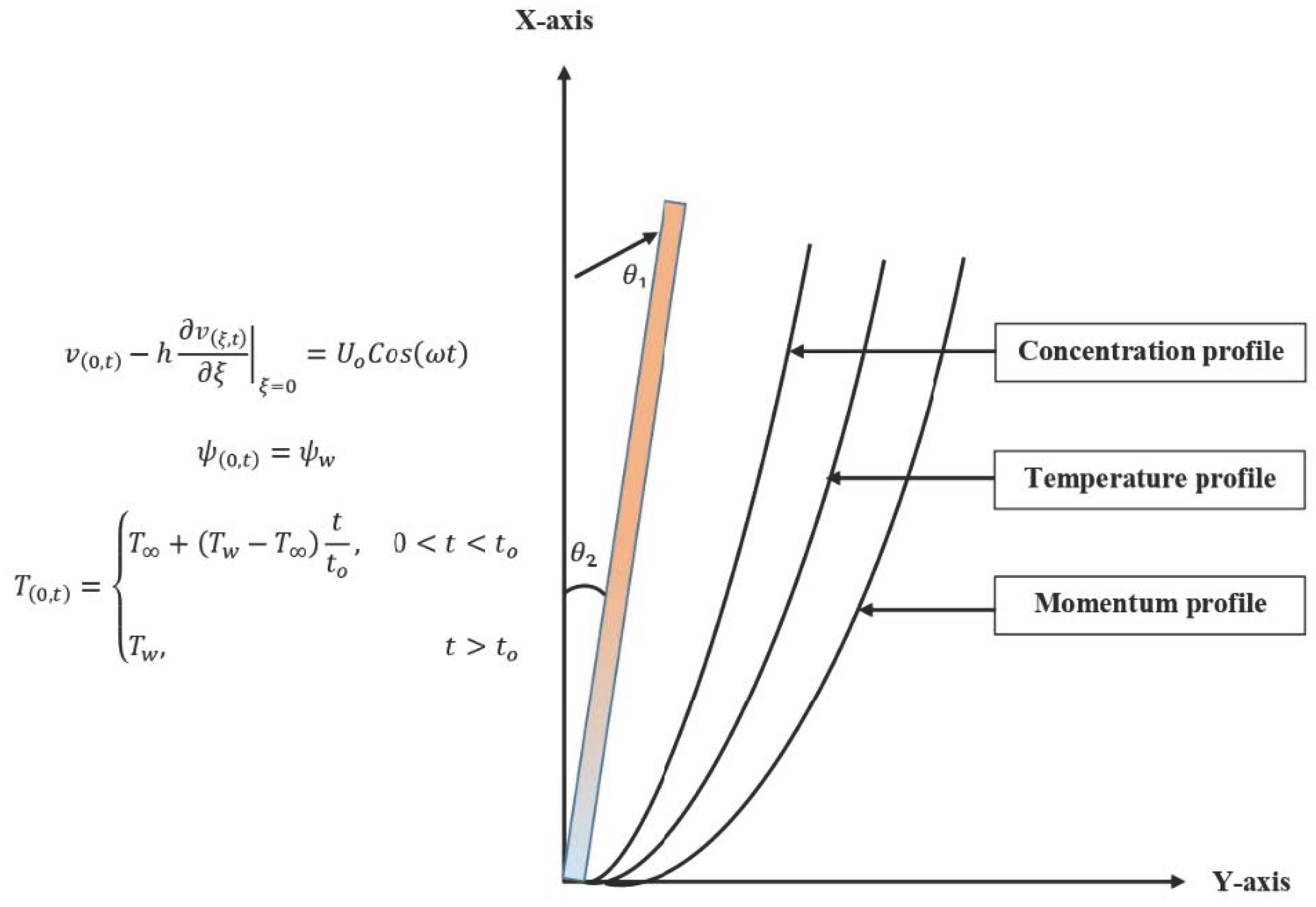
2. Problem Description

Suppose a laminar Oldroyd-B hybrid nanofluid flow on an oscillating pored infinite inclined plate with heat transfer. The flowing fluid is mixed with different types of nanoparticles $\left(Ag, Cu, Ti{O}_2\right)$ with water and engine oil as base fluid. In addition, its also supposed that the flowing fluid is electrically conducting, and an inclined magnetic field is applied with strength $B_o$. Furthermore, the slipping effect on the plate boundary and sinusoidal thermal conditions are also considered. At the start, both the plate and fluid are in a rest state with constant concentration ${\psi }_{\infty }$ and temperature $T_{\infty }$. After the passage of some time at $t>0^{+}$, the static hybrid suspension of different types of nanoparticles starts to move on the oscillating plate due to mixed convection, oscillations, and the inclination of the pored plate. The pored plate vibrates with some constant velocity $U_{o}Cos\left(\omega t\right)$ in which $\omega$ is the vibration rate of the inclined plane, as configured in Figure 1.

The basic partial differential equations are provided below, taking into account the following assumptions and ignoring the pressure gradient, viscous dissipation, and the use of Boussinseq’s and Rosseland approximations [36,37],

$$\begin{array}{ll}{\rho }_{nf}\left(1+{\mathsf{\Omega }}_1\frac{\partial }{\partial t}\right)\frac{\partial v_{\left(\xi ,t\right)}}{\partial t}& \\ & ={\mu }_{nf}\left(1+{\mathsf{\Omega }}_2\frac{\partial }{\partial t}\right)\frac{{\partial }^2{v}_{\left(\xi ,t\right)}}{\partial {\xi }^2}& \\ & -\left(1+{\mathsf{\Omega }}_1\frac{\partial }{\partial t}\right)\left(\sigma B_o^{2}sin\left({\theta }_1\right)+\frac{{\mu }_{nf}{\phi }_{nf}}{K}\right)v_{\left(\xi ,t\right)}& \\ & +g{\left(\rho {\beta }_T\right)}_{nf}Cos\left({\theta }_2\right)T_{\left(\xi ,t\right)}-g{\left(\rho {\beta }_T\right)}_{nf}Cos\left({\theta }_2\right)T_{\infty }& \\ & +g{\left(\rho {\beta }_C\right)}_{nf}Cos\left({\theta }_2\right){\psi }_{\left(\xi ,t\right)}-g{\left(\rho {\beta }_C\right)}_{nf}Cos\left({\theta }_2\right){\psi }_{\infty }\end{array}$$

(1)

$$\left(1+{\mathsf{\Omega }}_1\frac{\partial }{\partial t}\right){\tau }_{\left(\xi ,t\right)}={\mu }_{nf}\frac{\partial v_{\left(\xi ,t\right)}}{\partial \xi }$$

(2)

$${\left(\rho C_p\right)}_{nf}\frac{\partial T_{\left(\xi ,t\right)}}{\partial t}=-\frac{\partial {\delta }_{\left(\xi ,t\right)}}{\partial \xi }, {\delta }_{\left(\xi ,t\right)}=-k_{nf}\frac{\partial T_{\left(\xi ,t\right)}}{\partial \xi }$$

(3)

$$\frac{\partial {\psi }_{\left(\xi ,t\right)}}{\partial t}=-D_{nf}\frac{\partial J_{\left(\xi ,t\right)}}{\partial \xi }, J_{\left(\xi ,t\right)}=-\frac{\partial {\psi }_{\left(\xi ,t\right)}}{\partial \xi }$$

(4)

where all of the conditions and variables are given in the nomenclature portion. The following are the consistent conditions for momentum, concentration, and thermal equations:

$$v_{\left(\xi ,0\right)}=0, {\psi }_{\left(\xi ,0\right)}={\psi }_{\infty }, T_{\left(\xi ,0\right)}=T_{\infty }; \forall \xi \ge 0$$

(5)

$$v_{\left(0,t\right)}-h{\frac{\partial v_{\left(\xi ,t\right)}}{\partial \xi }|}_{\xi =0}=U_{o}Cos\left(\omega t\right), {\psi }_{\left(0,t\right)}={\psi }_w$$

$$T_{\left(0,t\right)}=\{\begin{array}{c}{T}_{\infty }+\left(T_w-T_{\infty }\right)\frac{t}{t_o}, 0<t<t_o\\ \\ \\ T_w, t>t_o\end{array}$$

(6)

$$v_{\left(\xi ,t\right)}\to 0, {\psi }_{\left(\xi ,t\right)}\to {\psi }_{\infty }, T_{\left(\xi ,t\right)}\to T_{\infty }; \xi \to \infty , t>0.$$

(7)

Now, to analyze the impact of all effecting parameters, introducing the following dimensionless variables, the related guided equations may be non-dimensionalized:

$$\begin{gathered} v^{*}=\frac{v}{U_o}, t^{*}=\frac{t}{t_o}, t_o=\frac{\nu }{U_o^2}, {\xi }^{*}=\frac{U_o}{\nu }\xi , T^{*}=\frac{T_{\left(\xi ,t\right)}-T_{\infty }}{T_{\infty }}, \\ {\psi }^{*}=\frac{C_{\left(\xi , t\right)}-C_{\infty }}{C_{\infty }}, {\delta }^{*}={\delta }_o, {\tau }^{*}=\frac{k}{h}\frac{\tau }{U_o\mu } \end{gathered}$$

By manipulating the above dimensionless variables in the governing Equations (1) to (4) along with boundary conditions (5) to (7) to overlooking the “*” symbols or notations, one acquires as follows:

$$\begin{array}{ll}{\mathsf{\Lambda }}_o\left(1+{\mathsf{\Omega }}_1\frac{\partial }{\partial t}\right)\frac{\partial v_{\left(\xi ,t\right)}}{\partial t}& \\ & ={\mathsf{\Lambda }}_1\left(1+{\mathsf{\Omega }}_2\frac{\partial }{\partial t}\right)\frac{{\partial }^2{v}_{\left(\xi ,t\right)}}{\partial {\xi }^2}-\left(1+{\mathsf{\Omega }}_1\frac{\partial }{\partial t}\right)\left(Msin\left({\theta }_1\right)+\frac{{\mathsf{\Lambda }}_1}{K}\right)v_{\left(\xi ,t\right)}+{\mathsf{\Lambda }}_{2}GrCos\left({\theta }_2\right)T_{\left(\xi ,t\right)}\\ & +{\mathsf{\Lambda }}_{3}GmCos\left({\theta }_2\right){\psi }_{\left(\xi ,t\right)}\end{array}$$

(8)

$$\left(1+{\mathsf{\Omega }}_1\frac{\partial }{\partial t}\right){\tau }_{\left(\xi ,t\right)}=\frac{\partial v_{\left(\xi ,t\right)}}{\partial \xi }$$

(9)

$${\mathsf{\Lambda }}_{4}Pr\frac{\partial T_{\left(\xi ,t\right)}}{\partial t}=-\frac{\partial {\delta }_{\left(\xi ,t\right)}}{\partial \xi }, {\delta }_{\left(\xi ,t\right)}=-{\mathsf{\Lambda }}_5\frac{\partial T_{\left(\xi ,t\right)}}{\partial \xi }$$

(10)

$${\mathsf{\Lambda }}_{6}Sc\frac{\partial {\psi }_{\left(\xi ,t\right)}}{\partial t}=-\frac{\partial J_{\left(\xi , t\right)}}{\partial \xi }, J_{\left(\xi ,t\right)}=-\frac{\partial {\psi }_{\left(\xi ,t\right)}}{\partial \xi }$$

(11)

With consistent dimensionless conditions,

$$v_{\left(\xi ,0\right)}=0, {\psi }_{\left(\xi ,0\right)}=0, T_{\left(\xi ,0\right)}=0; \forall \xi \ge 0$$

(12)

$$v_{\left(0,t\right)}-h{\frac{\partial v_{\left(\xi ,t\right)}}{\partial \xi }|}_{\xi =0}=Cos\left(\omega t\right), {\psi }_{\left(0,t\right)}=1, T_{\left(0,t\right)}=\{\begin{array}{c}t, 0<t\le 1\\ \\ \\ 1, t>1\end{array}$$

(13)

$$v_{\left(\xi , t\right)}\to 0, {\psi }_{\left(\xi , t\right)}\to 0, T_{\left(\xi , t\right)}\to 0; \xi \to \infty ,t>0$$

(14)

where $M,{\mathsf{\Omega }}_1,{\mathsf{\Omega }}_2,Gr,Gm,Pr,Sc,K$ are identified as the magnetic parameter, time relaxation, retardation parameter, heat Grashof number, mass Grashof number, Prandtl number, Schmidt number, and porosity parameter, respectively, whose mathematical forms are given below.

$$\begin{gathered} {\mathsf{\Lambda }}_o=\left(1-\phi \right)+\phi \frac{{\rho }_s}{{\rho }_f} ,{ \mathsf{\Lambda }}_1=\frac{1}{{\left(1-\phi \right)}^{2.5}} \\ {\mathsf{\Lambda }}_2=\left(1-\phi \right)+\frac{{\left(\rho {\beta }_T\right)}_s}{{\left(\rho {\beta }_T\right)}_f}, { \mathsf{\Lambda }}_3=\left(1-\phi \right)+\frac{{\left(\rho {\beta }_c\right)}_s}{{\left(\rho {\beta }_c\right)}_f},{ \mathsf{\Lambda }}_4 \\ =\left(1-\phi \right)+\frac{{\left(\rho C_p\right)}_s}{{\left(\rho C_p\right)}_f} \\ {\mathsf{\Lambda }}_5=\frac{k_s+2k_f-2\phi \left(k_f-k_s\right)}{k_s+2k_f+\phi \left(k_f-k_s\right)},M=\frac{{\sigma }^{*}k{B}_o^2}{{\mathrm{h}}^2\mu },\frac{1}{K}=\frac{\mathsf{\nu } {\phi }_1}{K^{*}{U}_o^2},Pr=\frac{{\nu }_f{C}_p}{k} \\ Gr=\frac{g{\beta }_T\nu T_{\infty }}{U_o^3},Gm=\frac{g{\beta }_c\nu C_{\infty }}{U_o^3},Sc=\frac{\nu }{D_f} \end{gathered}$$

Table 1. The quantities of nanofluids thermophysical properties.

Thermal Features	Regular Nanofluid	Hybrid Nanofluid
Density	${\rho }_f=\frac{{\rho }_{nf}}{\left(1-\phi \right)+\phi \frac{{\rho }_s}{{\rho }_s}}$	${\rho }_f=\frac{{\rho }_{hnf}}{\left(\left(1-{\phi }_2\right)\left(\left(1-{\phi }_1\right)+{\phi }_1\frac{{\rho }_{s1}}{{\rho }_f}\right)+{\phi }_2{\rho }_{s2}\right)}$
Dynamic Viscosity	${\mu }_f={\mu }_{nf}{\left(1-\phi \right)}^{2.5}$	${\mu }_f={\mu }_{hnf}{\left(1-{\phi }_1\right)}^{2.5}{\left(1-{\phi }_2\right)}^{2.5}$
Electrical conductivity	${\sigma }_f=\frac{{\sigma }_{nf}}{\left(1+\frac{3\left(\frac{{\sigma }_s}{{\sigma }_f}-1\right)\phi }{\left(\frac{{\sigma }_s}{{\sigma }_f}+2\right)-\left(\frac{{\sigma }_s}{{\sigma }_f}-1\right)\phi }\right)}$	${\sigma }_{bf}=\frac{{\sigma }_{hnf}}{\left(1+\frac{3\phi \left({\phi }_1{\sigma }_1+{\phi }_2{\sigma }_2-{\sigma }_{bf}\left({\phi }_1+{\phi }_2\right)\right)}{\left({\phi }_1{\sigma }_1+{\phi }_2{\sigma }_2+2\phi {\sigma }_{bf}-\phi {\sigma }_{bf}\left({\phi }_1{\sigma }_1+{\phi }_2{\sigma }_2-{\sigma }_{bf}\left({\phi }_1+{\phi }_2\right)\right)\right)}\right)}$
Thermal conductivity	$k_f=\frac{k_{nf}}{\left(\frac{k_s+\left(n-1\right)k_f-\left(n-1\right)\left(k_f-k_s\right)\phi }{k_s+\left(n-1\right)k_f+\left(k_f-k_s\right)\phi }\right)}$	$k_{bf}=\frac{k_{hnf}}{\left(\frac{k_{s2}+\left(n-1\right)k_{bf}-\left(n-1\right)\left(k_{bf}-k_{s2}\right){\phi }_2}{k_{s2}+\left(n-1\right)k_{bf}+\left(k_{bf}-k_{s2}\right){\phi }_2}\right)}$ and $k_f=\frac{k_{bf}}{\left(\frac{k_{s1}+\left(n-1\right)k_f-\left(n-1\right)\left(k_f-k_{s1}\right){\phi }_1}{k_{s1}+\left(n-1\right)k_f+\left(k_f-k_{s1}\right){\phi }_1}\right)}$
Heat capacitance	${\left(\rho C_p\right)}_f=\frac{{\left(\rho C_p\right)}_{nf}}{\left(1-\phi \right)+\phi \frac{{\left(\rho C_p\right)}_s}{{\left(\rho C_p\right)}_f}}$	${\left(\rho C_p\right)}_s=\frac{{\left(\rho C_p\right)}_{hnf}}{\left(1-{\phi }_2\right)\left(\left(1-{\phi }_1\right)+{\phi }_1\frac{{\left(\rho C_p\right)}_{s1}}{{\left(\rho C_p\right)}_f}\right)+{\phi }_2{\left(\rho C_p\right)}_{s2}}$
Thermal Expansion Coefficient	${\left(\rho \beta \right)}_f=\frac{{\left(\rho \beta \right)}_{nf}}{\left(1-\phi \right)+\phi \frac{{\left(\rho \beta \right)}_s}{{\left(\rho \beta \right)}_f}}$	${\left(\rho \beta \right)}_f=\frac{{\left(\rho \beta \right)}_{hnf}}{\left(1-{\phi }_2\right)\left(\left(1-{\phi }_1\right)+{\phi }_1\frac{{\left(\rho \beta \right)}_{s1}}{{\left(\rho \beta \right)}_{f1}}\right)+{\phi }_2{\left(\rho \beta \right)}_{s2}}$

and

Table 2. The thermal features of nanoparticles and regular fluids.

Material	Water	Engine Oil	Ag	Cu	TiO2
$\mathsf{\rho }\left(\mathrm{kg}/{\mathrm{m}}^3\right)$	997.1	884	10,500	8933	4250
${\mathrm{C}}_{\mathrm{p}}\left(\mathrm{J}/\mathrm{kg} \mathrm{K}\right)$	4179	1910	235	385	686.2
$\mathrm{k}\left(\mathrm{W}/\mathrm{m} \mathrm{K}\right)$	0.613	0.144	429	401	8.9528
${\mathsf{\beta }}_{\mathrm{T}}\times {10}^{-5}\left({\mathrm{K}}^{-1}\right)$	21	70	1.89	1.67	0.90

summarize the thermal properties of the hybrid nanofluid model, base material, and solid nanoparticles. Furthermore, for such thermal models, the particle’s solid volume fraction, hybrid nanofluid, mercury, copper, titanium dioxide, the nanofluid, and actual base liquid are reflected by $h_{nf}, Ag, Cu, Ti{O}_2, nf, f$, respectively.

3. Basic Preliminaries

The regularized Prabhakar fractional derivative operator ${}_{ }{}^C\mathfrak{D}{}_{\alpha ,\beta ,\alpha }^{\gamma }$ for a continuous function $h\left(t\right)$ is defined as,

$${}_{ }{}^C\mathfrak{D}{}_{\alpha ,\beta ,\alpha }^{\gamma }h\left(t\right)=E_{\alpha ,m-\beta ,\alpha }^{-\gamma }{h}^m\left(t\right)={{\displaystyle \int }}_0^t{\left(t-\tau \right)}^{m-\beta -1}{E}_{\alpha ,m-\beta }^{-\gamma }\left(\alpha {\left(t-\tau \right)}^{\alpha }\right)h^m\left(\tau \right)d\left(\tau \right)$$

where,

$$E_{\alpha ,\beta ,\alpha }^{\gamma }\mathrm{h}\left(t\right)={{\displaystyle \int }}_0^t{\left(t-\tau \right)}^{\beta -1}{E}_{\alpha ,\beta }^{\gamma }\left(\alpha {\left(t-\tau \right)}^{\alpha }\right)\mathrm{h}\left(\tau \right)d\left(\tau \right)$$

Is the Prabhakar integral, and,

$$E_{\alpha ,\beta }^{\gamma }\left(z\right)={\displaystyle \sum }_{n=0}^{\infty }\frac{\mathsf{\Gamma }\left(\gamma +n\right)z^n}{n!\mathsf{\Gamma }\left(\gamma \right)\mathsf{\Gamma }{\left(\alpha n+\beta \right)}^{\prime }},\alpha , \beta , \gamma ϵℂ, Re\left(\alpha \right)>0$$

Is known as the three-parameter Mittage-Leffler function and ${}_{ }{}^C\mathfrak{D}{}_{\alpha ,\beta ,\alpha }^{\gamma }$ signifies the Prabhakar derivative operator with $\alpha , \beta , \gamma ϵℂ, Re\left(\alpha \right)>0$. The LT of regularized Prabhakar derivative may be developed as.

$$ℒ\left\{{}_{ }{}^C\mathfrak{D}{}_{\alpha ,\beta ,\alpha }^{\gamma }h\left(t\right)\right\}=q^{\beta -m}{\left(1-\alpha q^{-\alpha }\right)}^{\gamma }ℒ\left\{h^m\left(t\right)\right\}$$

(15)

Here $\alpha ,\beta , \gamma$ represent the Prabhakar fractional constraints, and $q$ is the Laplace transformed variable. In this study, we used an efficient and current mathematical fractional approach, from which we may also infer the effect of thermal memory. So, in this section, we will become acquainted with the derivative of Prabhakar fractional, which is primarily based on generalized Fourier’s and Fick’s laws of thermal conductivity

$${\delta }_{\left(\xi ,t\right)}=-k_{nf}{}_{ }{}^C\mathfrak{D}{}_{\alpha ,\beta ,\alpha }^{\gamma }\frac{\partial T_{\left(\xi ,t\right)}}{\partial \xi }$$

(16)

$$J_{\left(\xi ,t\right)}=-{}_{ }{}^C\mathfrak{D}{}_{\alpha ,\beta ,\alpha }^{\gamma }\frac{\partial {\psi }_{\left(\xi ,t\right)}}{\partial \xi }$$

(17)

where $k_{nf}$ is the generalized thermal conductivity and ${}_{ }{}^C\mathfrak{D}{}_{\alpha ,\beta ,\alpha }^{\gamma }$ is well known as Prabhakar fractional derivative.

4. Solution of the Problem

The fractional modeling of guided equations using the Prabhakar-fractional description and the solution of the associated fractional model will be carried out in this framework, with their respective converted physical conditions.

4.1. Concentration Profile

For the solution of fractional systems, many strategies have been utilized. However, in this work, we selected the integral transform approach, called Laplace transformation (LT), by implementing the LT to fractional Equations (11) and (17) for the concentration solution profile.

$${\mathsf{\Lambda }}_{6}Sc s{\overline{\psi }}_{\left(\xi ,s\right)}=-\frac{\partial {\overline{J}}_{\left(\xi ,s\right)}}{\partial \xi }$$

(18)

$${\overline{J}}_{\left(\xi ,s\right)}=-s^{\beta }{\left(1-\alpha s^{-\alpha }\right)}^{\gamma }\frac{\partial {\overline{\psi }}_{\left(\xi ,s\right)}}{\partial \xi }$$

(19)

$${\overline{\psi }}_{\left(\xi ,s\right)}=\frac{1}{s}, {\overline{\psi }}_{\left(\infty ,s\right)}=0$$

Inserting Equation (13) into Equation (12), we acquire,

$${\overline{\psi }}_{\left(\xi ,s\right)}=\frac{1}{s}{e}^{-\xi \sqrt{\frac{{\mathsf{\Lambda }}_6 Sc s}{s^{\beta }{\left(1-\alpha s^{-\alpha }\right)}^{\gamma }}}}$$

(20)

The Laplace inverse of the above-attained solution will be analyzed numerically by employing Stehfest and Tzou’s algorithms in

Table 3. Numerical comparison of thermal, concentration, and momentum pro-files.

$\mathit{\xi }$	${\mathit{T}}_{\left(\mathit{\xi },\mathit{t}\right)} \mathbf{by}$ Tzous	${\mathit{T}}_{\left(\mathit{\xi },\mathit{t}\right)} \mathbf{by}$ Stehfest	${\mathit{\psi }}_{\left(\mathit{\xi },\mathit{t}\right)} \mathbf{by}$ Tzous	${\mathit{\psi }}_{\left(\mathit{\xi },\mathit{t}\right)} \mathbf{by}$ Stehfest	${\mathit{V}}_{\left(\mathit{\xi },\mathit{t}\right)} \mathbf{by}$ Tzous	${\mathit{V}}_{\left(\mathit{\xi },\mathit{t}\right)} \mathbf{by}$ Stehfest
0.1	0.8847	0.8893	0.9356	0.9376	0.6252	0.6140
0.3	0.7177	0.7216	0.8214	0.8242	0.5969	0.5852
0.5	0.5822	0.5855	0.7204	0.7245	0.5645	0.5338
0.7	0.4722	0.4754	0.6318	0.5597	0.4840	0.4727
0.9	0.3831	0.3854	0.5540	0.5597	0.4020	0.4096
1.1	0.3107	0.3126	0.4558	0.4919	0.3590	0.3493
1.3	0.2520	0.2536	0.4260	0.4324	0.3028	0.2940
1.5	0.2044	0.2057	0.3735	0.3800	0.2529	0.2450
1.7	0.1658	0.1669	0.3275	0.3340	0.2094	0.2025
1.9	0.1344	0.1354	0.2872	0.3935	0.1722	0.1662

and

Table 4. Numerical values of the skin friction, the Sherwood number, and the Nusselt number at different times.

$\mathit{\alpha }$	$\mathit{N}\mathit{u}$$\mathbf{at} \mathit{t}=1.0$	$\mathit{N}\mathit{u}$$\mathbf{at} \mathit{t}=1.5$	$\mathit{S}\mathit{h}$$\mathbf{at} \mathit{t}=1.0$	$\mathit{S}\mathit{h}$$\mathbf{at} \mathit{t}=1.5$	${\mathit{C}}_{\mathit{f}}$$\mathbf{at} \mathit{t}=1.0$	${\mathit{C}}_{\mathit{f}}$$\mathbf{at} \mathit{t}=1.0$
0.1	0.8386	0.7829	0.4927	0.4456	0.1371	0.0105
0.2	0.8739	0.8268	0.5211	0.4779	0.1317	0.0130
0.3	0.9094	0.8806	0.5560	0.5256	0.1254	0.0155
0.4	0.9430	0.9427	0.5960	0.5936	0.1181	0.0180
0.5	0.9726	1.0094	0.6383	0.6852	0.1093	0.0209
0.6	0.9965	1.0759	0.6795	0.7999	0.0982	0.0237
0.7	1.0140	1.1375	0.7166	0.9323	0.0839	0.0265
0.8	1.0252	1.1904	0.7373	1.0732	0.0633	0.0295
0.9	1.0306	1.2327	0.7708	1.2127	0.0280	0.0325

.

4.2. Solution of Temperature Field

The temperature field is solved using the Laplace technique on second-order partial differential Equations (10) and (16) and their matching conditions.

$${\mathsf{\Lambda }}_4\mathrm{Pr}s{\overline{T}}_{\left(\xi ,s\right)}=-\frac{\partial {\overline{\delta }}_{\left(\xi ,s\right)}}{\partial \xi }$$

(21)

$${\overline{\delta }}_{\left(\xi ,s\right)}=-{\mathsf{\Lambda }}_5{s}^{\beta }{\left(1-\alpha s^{-\alpha }\right)}^{\gamma }\frac{\partial {\overline{T}}_{\left(\xi ,s\right)}}{\partial \xi }$$

(22)

With,

$${\overline{T}}_{\left(0,s\right)}=\frac{1-e^{-s}}{s^2}, {\overline{T}}_{\left(\infty ,s\right)}=0$$

we acquire,

$${\overline{T}}_{\left(y,s\right)}=\frac{1-e^{-s}}{s^2}{e}^{-\xi \sqrt{\frac{{\mathsf{\Lambda }}_{4}Pr}{{\mathsf{\Lambda }}_5}\frac{s^{1-\beta }}{{\left(1-\alpha s^{-\alpha }\right)}^{\gamma }}}}$$

(23)

Yet again, using the Laplace inverse of the above equation will be numerically analyzed in Table 2 and Table 3.

4.3. Solution of the Velocity Field

In this segment, the solution of the velocity equation will be derived by pertaining the LT on second-order PDE Equation (8), and with Equation (15), we procure a differential equation that is not homogeneous.

$$\frac{{\partial }^2{\overline{v}}_{\left(\xi ,s\right)}}{\partial {\xi }^2}-\frac{\left(1+{\mathsf{\Omega }}_{1}s\right)}{{\mathsf{\Lambda }}_1\left(1+{\mathsf{\Omega }}_{2}s\right)}\left(Msin\left({\theta }_1\right)+\frac{{\mathsf{\Lambda }}_1}{K}+{\mathsf{\Lambda }}_{o}s\right){\overline{v}}_{\left(\xi ,s\right)}=-\frac{{\mathsf{\Lambda }}_{2}GrCos\left({\theta }_2\right)}{{\mathsf{\Lambda }}_1\left(1+{\mathsf{\Omega }}_{2}s\right)}{\overline{T}}_{\left(\xi ,s\right)}-\frac{{\mathsf{\Lambda }}_{3}GmCos\left({\theta }_2\right)}{{\mathsf{\Lambda }}_1\left(1+{\mathsf{\Omega }}_{2}s\right)}{\overline{\psi }}_{\left(\xi ,s\right)}$$

(24)

with conditions,

$${\overline{v}}_{\left(0,s\right)}-h{\frac{\partial {\overline{v}}_{\left(\xi ,s\right)}}{\partial \xi }|}_{\xi =0}=\frac{s}{s^2+{\omega }^2}; {\overline{v}}_{\left(\xi ,s\right)}\to 0 as \xi \to \infty$$

Using the matching conditions, we obtain the solution to Equation (24) as follows:

$$\begin{array}{cc}\hfill & {\overline{v}}_{(\xi ,s)}=\frac{1}{1+h\sqrt{\frac{\left(1+{\mathsf{\Omega }}_{1}s\right)}{{\mathsf{\Lambda }}_1\left(1+{\mathsf{\Omega }}_{2}s\right)}\left(MSin\left({\theta }_1\right)+\frac{{\mathsf{\Lambda }}_1}{K}+{\mathsf{\Lambda }}_{o}s\right)}}\hfill \\ \hfill & \left(\frac{{\mathsf{\Lambda }}_{2}GrCos\left({\theta }_2\right)}{{\mathsf{\Lambda }}_1\left(1+{\mathsf{\Omega }}_{2}s\right)}\frac{1-{\mathrm{e}}^{-s}}{s^2}\frac{1+h\sqrt{\frac{{\mathsf{\Lambda }}_{4}Pr}{{\mathsf{\Lambda }}_5}\frac{s^{1-\beta }}{{\left(1-\alpha s^{-\alpha }\right)}^{\gamma }}}}{\left(\frac{{\mathsf{\Lambda }}_{4}Pr}{{\mathsf{\Lambda }}_5}\frac{s^{1-\beta }}{{\left(1-\alpha s^{-\alpha }\right)}^{\gamma }}\right)-\frac{\left(1+{\mathsf{\Omega }}_{1}s\right)}{{\mathsf{\Lambda }}_1\left(1+{\mathsf{\Omega }}_{2}s\right)}\left(MSin\left({\theta }_1\right)+\frac{{\mathsf{\Lambda }}_1}{K}+{\mathsf{\Lambda }}_{o}s\right)}\right.\hfill \\ \hfill & +\frac{{\mathsf{\Lambda }}_{3}GmCos\left({\theta }_2\right)}{{\mathsf{\Lambda }}_1\left(1+{\mathsf{\Omega }}_{2}s\right)s}\frac{1+h\sqrt{\frac{{\mathsf{\Lambda }}_{6}Scs}{s^{\beta }{\left(1-\alpha s^{-\alpha }\right)}^{\gamma }}}}{\left(\frac{{\mathsf{\Lambda }}_{6}Scs}{s^{\beta }{\left(1-\alpha s^{-\alpha }\right)}^{\gamma }}\right)-\frac{\left(1+{\mathsf{\Omega }}_{1}s\right)}{{\mathsf{\Lambda }}_1\left(1+{\mathsf{\Omega }}_{2}s\right)}\left(MSin\left({\theta }_1\right)+\frac{{\mathsf{\Lambda }}_1}{K}+{\mathsf{\Lambda }}_{o}s\right)}\hfill \\ \hfill & \left.+\frac{s}{s^2+{\omega }^2}\right)e^{-\xi \sqrt{\frac{\left(1+{\mathsf{\Omega }}_{1}s\right)}{{\mathsf{\Lambda }}_1\left(1+{\mathsf{\Omega }}_{2}s\right)}\left(MSin\left({\theta }_1\right)+\frac{{\mathsf{\Lambda }}_1}{K}+{\mathsf{\Lambda }}_{o}s\right)}}\hfill \\ \hfill & -\frac{{\mathsf{\Lambda }}_{2}GrCoS\left({\theta }_2\right)}{{\mathsf{\Lambda }}_1\left(1+{\mathsf{\Omega }}_{2}s\right)}\frac{1-{\mathrm{e}}^{-s}}{s^2}\frac{e^{-\xi \sqrt{\frac{{\mathsf{\Lambda }}_4{P}_r{s}^{1-\beta }}{{\mathsf{\Lambda }}_5{\left(1-\alpha s^{-\alpha }\right)}^{\gamma }}}}}{\left(\frac{{\mathsf{\Lambda }}_{4}Pr}{{\mathsf{\Lambda }}_5}\frac{s^{1-\beta }}{{\left(1-\alpha s^{-\alpha }\right)}^{\gamma }}\right)-\frac{\left(1+{\mathsf{\Omega }}_{1}s\right)}{{\mathsf{\Lambda }}_1\left(1+{\mathsf{\Omega }}_{2}s\right)}\left(MSin\left({\theta }_1\right)+\frac{{\mathsf{\Lambda }}_1}{K}+{\mathsf{\Lambda }}_{o}s\right)}\hfill \\ \hfill & -\frac{{\mathsf{\Lambda }}_{3}GmCos\left({\theta }_2\right)}{{\mathsf{\Lambda }}_1\left(1+{\mathsf{\Omega }}_{2}s\right)s}\frac{e^{-\xi \sqrt{\frac{{\mathsf{\Lambda }}_{6}Scs}{s\beta \left(1-\alpha s^{-\alpha }\gamma \right.}}}}{\left(\frac{{\mathsf{\Lambda }}_{6}Scs}{s^{\beta }{\left(1-\alpha s^{-\alpha }\right)}^{\gamma }}\right)-\frac{\left(1+{\mathsf{\Omega }}_{1}s\right)}{{\mathsf{\Lambda }}_1\left(1+{\mathsf{\Omega }}_{2}s\right)}\left(MSin\left({\theta }_1\right)+\frac{{\mathsf{\Lambda }}_1}{K}+{\mathsf{\Lambda }}_{o}s\right)}\hfill \end{array}$$

(25)

The attained solutions of thermal, concentration, and momentum profiles are complicated to solve analytically. Different authors have utilized different numerical techniques, so we have also used numerical algorithms for the Laplace inverse, namely Stehfest and Tzou’s numerical schemes. The mathematical form of these algorithms can be described as [38,39,40],

$$\begin{gathered} w\left(\xi ,t\right)=\frac{ln\left(2\right)}{t}{\displaystyle \sum }_{n=1}^N{v}_n\overline{w}\left(\xi ,n\frac{ln\left(2\right)}{t}\right) \\ {v}_n={\left(-1\right)}^{n+\frac{N}{2}}{\displaystyle \sum }_{r=\left[\frac{q+1}{2}\right]}^{min\left(q,\frac{N}{2}\right)}\frac{r^{\frac{N}{2}}\left(2r\right)!}{\left(\frac{N}{2}-r\right)!r! \left(r-1\right)! \left(q-r\right)! \left(2r-q\right)!} \end{gathered}$$

In addition,

$$w\left(\xi ,t\right)=\frac{e^{4.7}}{t}\left[\frac{1}{2}\overline{w}\left(r,\frac{4.7}{t}\right)+Re\left\{{\displaystyle \sum }_{j=1}^N{\left(-1\right)}^k\overline{w}\left(r,\frac{4.7+k\pi i}{t}\right)\right\}\right]$$

4.3.1. Limiting Cases

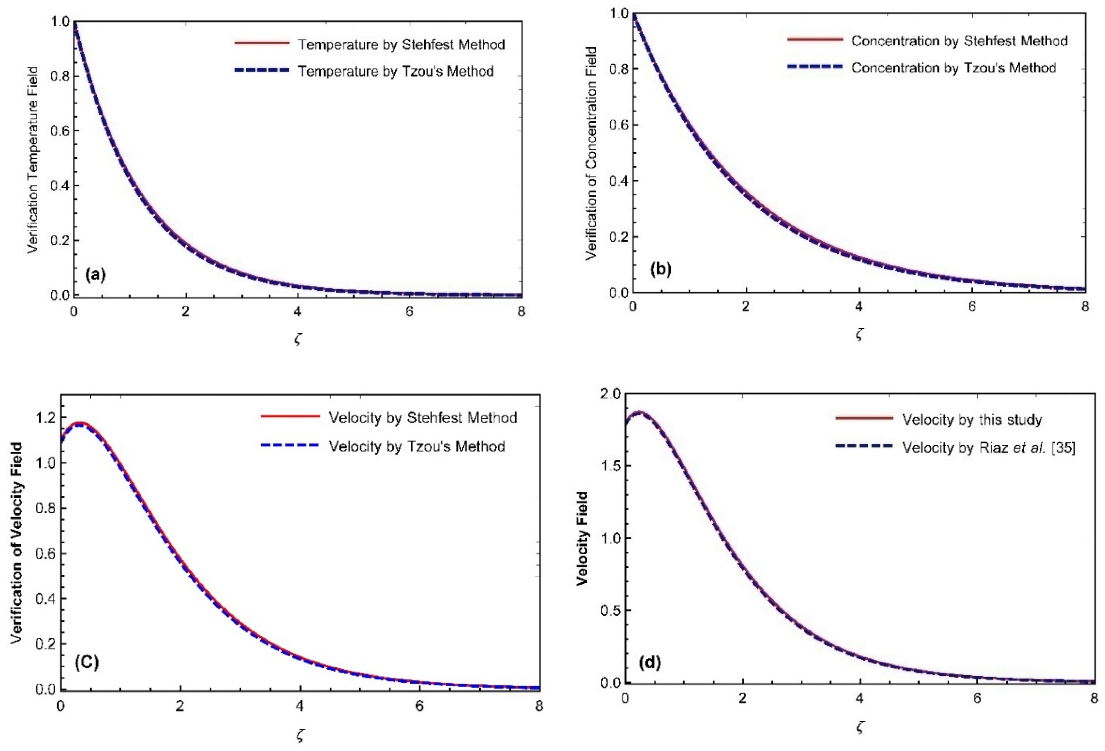
The above-achieved solution of the profile of velocity can be transmuted into a fractional Maxwell fluid model as attained by Ghalib et al. [41] by inserting ${\mathsf{\Omega }}_2=0$ into Equation (25), then the momentum profile will become as,

$${\overline{v}}_{\left(\xi ,s\right)}=\frac{1}{1+h\sqrt{\frac{\left(1+{\mathsf{\Omega }}_{1}s\right)}{{\mathsf{\Lambda }}_1}\left(MSin\left({\theta }_1\right)+\frac{{\mathsf{\Lambda }}_1}{K}+{\mathsf{\Lambda }}_{o}s\right)}}$$

$$\begin{array}{cc}\hfill & \left(\frac{{\mathsf{\Lambda }}_{2}GrCos\left({\theta }_2\right)}{{\mathsf{\Lambda }}_1}\frac{1-{\mathrm{e}}^{-s}}{s^2}\frac{1+h\sqrt{\frac{{\mathsf{\Lambda }}_{4}Pr}{{\mathsf{\Lambda }}_5}\frac{s^{1-\beta }}{{\left(1-\alpha s^{-\alpha }\right)}^{\gamma }}}}{\left(\frac{{\mathsf{\Lambda }}_{4}Pr}{{\mathsf{\Lambda }}_5}\frac{s^{1-\beta }}{{\left(1-\alpha s^{-\alpha }\right)}^{\gamma }}\right)-\frac{\left(1+{\mathsf{\Omega }}_{1}s\right)}{{\mathsf{\Lambda }}_1}\left(MSin\left({\theta }_1\right)+\frac{{\mathsf{\Lambda }}_1}{K}+{\mathsf{\Lambda }}_{o}s\right)}\right.\hfill \\ \hfill & +\frac{{\mathsf{\Lambda }}_{3}GmCos\left({\theta }_2\right)}{{\mathsf{\Lambda }}_{1}s}\frac{1+h\sqrt{\frac{{\mathsf{\Lambda }}_{6}Scs}{s^{\beta }{\left(1-\alpha s^{-\alpha }\right)}^{\gamma }}}}{\left(\frac{{\mathsf{\Lambda }}_{6}Scs}{s^{\beta }{\left(1-\alpha s^{-\alpha }\right)}^{\gamma }}\right)-\frac{\left(1+{\mathsf{\Omega }}_{1}s\right)}{{\mathsf{\Lambda }}_1}\left(MSin\left({\theta }_1\right)+\frac{{\mathsf{\Lambda }}_1}{K}+{\mathsf{\Lambda }}_{o}s\right)}\hfill \\ \hfill & \left.+\frac{s}{s^2+{\omega }^2}\right)e^{-\xi \sqrt{\frac{\left(1+{\mathsf{\Omega }}_{1}s\right)}{{\mathsf{\Lambda }}_1}\left(MSin\left({\theta }_1\right)+\frac{{\mathsf{\Lambda }}_1}{K}+{\mathsf{\Lambda }}_{o}s\right)}}\hfill \\ \hfill & -\frac{{\mathsf{\Lambda }}_{2}GrCos\left({\theta }_2\right)}{{\mathsf{\Lambda }}_1}\frac{1-{\mathrm{e}}^{-s}}{s^2}\frac{e^{-\xi \sqrt{\frac{{\mathsf{\Lambda }}_4{P}_r{s}^{1-\beta }}{{\mathsf{\Lambda }}_5{\left(1-\alpha s^{-\alpha }\right)}^{\gamma }}}}}{\left(\frac{{\mathsf{\Lambda }}_{4}Pr}{{\mathsf{\Lambda }}_5}\frac{s^{1-\beta }}{{\left(1-\alpha s^{-\alpha }\right)}^{\gamma }}\right)-\frac{\left(1+{\mathsf{\Omega }}_{1}s\right)}{{\mathsf{\Lambda }}_1}\left(MSin\left({\theta }_1\right)+\frac{{\mathsf{\Lambda }}_1}{K}+{\mathsf{\Lambda }}_{o}s\right)}\hfill \\ \hfill & -\frac{{\mathsf{\Lambda }}_{3}GmCos\left({\theta }_2\right)}{{\mathsf{\Lambda }}_{1}s}\frac{e^{-\xi \sqrt{\frac{{\mathsf{\Lambda }}_{6}Scs}{s^{\beta }\left(1-\alpha s^{-\alpha }\gamma \right.}}}}{\left(\frac{{\mathsf{\Lambda }}_{6}Scs}{s^{\beta }{\left(1-\alpha s^{-\alpha }\right)}^{\gamma }}\right)-\frac{\left(1+{\mathsf{\Omega }}_{1}s\right)}{{\mathsf{\Lambda }}_1}\left(MSin\left({\theta }_1\right)+\frac{{\mathsf{\Lambda }}_1}{K}+{\mathsf{\Lambda }}_{o}s\right)}\hfill \end{array}$$

(26)

Similarly, the solution attained of the velocity field in Equation (25) can be transformed into the attained results of Talha et al. in [14] by taking $f\left(t\right)=Cos\left(\omega t\right)=0$, which validates the attained solution of this work.

4.3.2. Validity

The comparison, including both numerical techniques, Stehfest and Tzou’s, was examined by drawing Figure 2a–d for thermal, concentration, and momentum profiles. The results from both curves have a slight overlap. In Figure 2d, a comparison of both numerical models and strategies for velocity fields using the Prabhakar fractional method is displayed with the work of Riaz et al. [42]. The calculations gained by using the Prabhakar fractional framework have an adequate accuracy compared to the exploration of Riaz et al. [42].

5. Discussion of Results

This paper examines an Oldroyd-B hybrid nanofluid on a pored oscillating plate under the magnetic impact, slipping effect, and sinusoidal heating conditions by exploiting a newly introduced and effective mathematical method, Prabhakar fractional operator, which has a Mittag-Leffler kernel in its constitutive equations. The physical impact of flow parameters, i.e., fractional constraints, Prandtl number, thermal Grashof and mass Groshof numbers, time relaxation and retardation parameters, Schmidt number, volume fraction, porosity and magnetic parameters, and angle of magnetic fields’ inclination are utilized to discourse the physical understanding of the obtained results for concentration, momentum, and thermal profiles in Figure 2, Figure 3, Figure 4, Figure 5, Figure 6, Figure 7, Figure 8, Figure 9 and Figure 10.

Figure 3 depicts the influence of fractional parameters and Pr on the temperature field. The computations expose that rate of temperature declines by moving the fractional parameters values as well as Pr. It’s to be seen that the temperature for silver-based nanofluid has a relatively higher value than copper-based nanofluid. Figure 4 portrays the impact of fractional parameters (β, α, and γ) and Sc on the concentration. It is exposed that the concentration rate declines by varying the estimations of fractional parameters as well as Sc. Moreover, it’s noted that the concentration profile for silver-based nanofluid has a relatively higher value than copper-based nanofluid. Figure 5a shows that the velocity field declines as fractional parameters are increased. Furthermore, the velocity profile for silver-based nanofluid has a relatively higher value than copper-based nanofluid. Figure 5b reveals the impact of fractional parameters on velocity profile in the existence of slip conditions and considers the slip constraint estimation to be zero. This figure shows that velocity decay agrees with significant fractional parameter estimations. Moreover, there is a prominent fast growth in velocity on the profile through the condition of slip associated with the slip constraint. Figure 6a,b represent the impact of the ${\mathsf{\Omega }}_1$ and ${\mathsf{\Omega }}_2$ on the velocity profile. It is found that the increase in velocity for growing the estimations of ${\mathsf{\Omega }}_1$ but a decrease in velocity has seemed to enhance the estimations of ${\mathsf{\Omega }}_2$. In fact, a rise in ${\mathsf{\Omega }}_1$, declined the fluid’s thickness so that it will hasten the speed of the liquid and velocity increases. Moreover, the growth of ${\mathsf{\Omega }}_2$ which guides to an increase in the outline layer viscosity and lessening the fluid velocity. It is portrayed that the impact of ${\mathsf{\Omega }}_1$ and ${\mathsf{\Omega }}_2$ on velocity are relatively reverse.

Figure 7a illustrates the velocity to evaluate the influence of Gr. An increase in velocity field is observed for enhancing the estimation of Gr. Substantially, the rise in Gr, which is the effect of more encouraging fluid flows, is due to growth in buoyancy effects. Consequently, these forces can influence increasing the velocity. Figure 7b demonstrate the momentum field to evaluate the influence of Gm. An augment in the velocity is observed for enhancing the estimation of Gm. Physically, the mass Grashof number exemplifies the ratio of the buoyant force to the viscous force of hydrodynamic. As typical, the fluid velocity rises, and the peak value is more distinctive owing to an improvement in the species’ buoyant force. Figure 8a denoted the impact of Pr on momentum profile and noted that the moving fluid’s velocity improvements in Pr decay. The outline velocity layer gains thicker because of the lower thermal diffusion rate, Pr governs the relative viscosity of momentum boundary layers in thermal transmission problems. Figure 8b shows that the velocity profile is also inversely proportional to the Sc because as the estimations of Sc rise, it grows kinematic viscosity and declines mass diffusivity. Figure 9a displays the temperature field for various estimations of nanoparticle volume fraction when the other constraints are fixed. It is detected that the velocity of the nanofluid growths with the growing volume of a fraction of nanoparticles because by growing values of volume fraction pointing that thickness of thermal boundary layer is reduced. This highlights that fluid becomes more viscous with the rise in volume fraction. The fluid velocity is increased by growing the estimations of K, as observed in Figure 9b. The impact of magnetic field M is deliberated in Figure 10a, and noted that the velocity is reduced by swelling the value of M because of Lorentz forces. It is a form of resistant force that supports the velocity decline. The velocity is inversely proportional to the angle of inclination ${\theta }_1$ which is seen in Figure 10b. Moreover, it’s prominent that the temperature, concentration, and momentum profiles for silver-based nanofluid have a relatively higher value than copper-based nanofluid.

6. Conclusions

This study examines the investigations of convection Oldroyd-B nanofluid model flowing fluid on an incline poured oscillating plate under the impact of an incline magnetic field. In order to account for generalized effects of memory, a fractional model was proposed using the recently announced Mittag-Leffler kernel and Prabhakar fractional operator in the governing equations. The research given in this article is entirely new. This model introduces fractionalized diffusion and thermal equations by combining Prabhakar’s fractional operator with generalized Fick’s and Fourier’s laws. The solution of the non-integer Prabhakar-like fractional model is attained by employing the numerical technique, namely the Laplace transformation scheme. Finally, the impact of different parameters and comparisons is plotted to evaluate the physical interpretation of the attained results of governed equations. The primary outcomes can be encapsulated as follows:

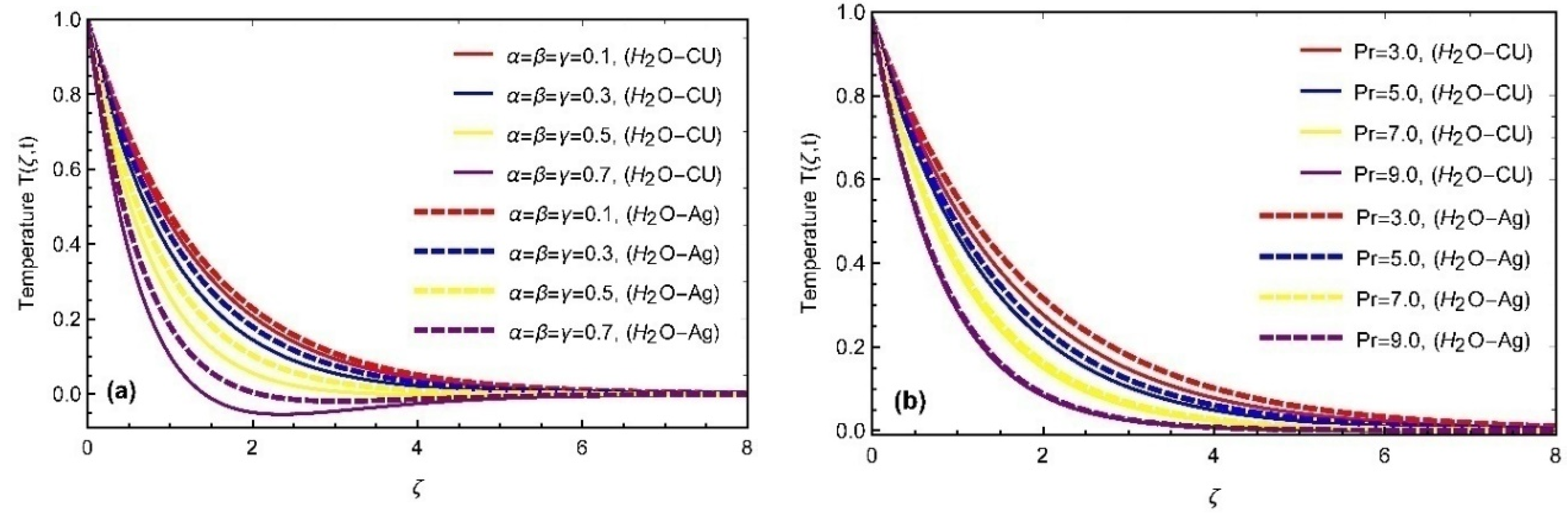
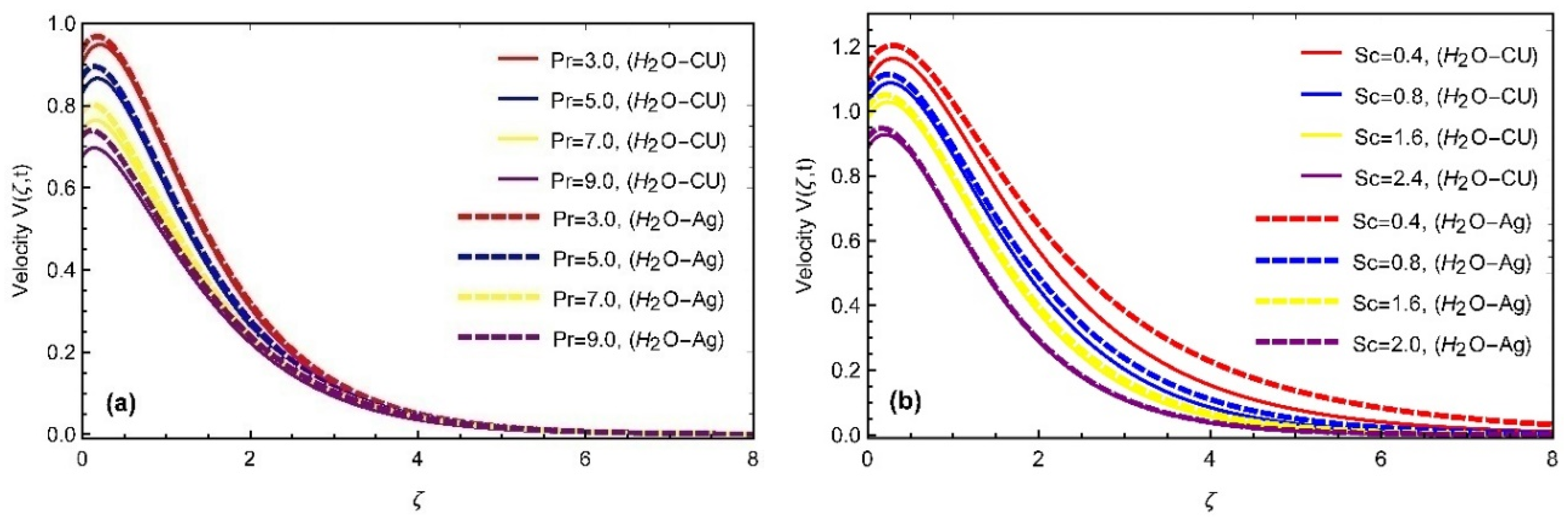
• The heat transfer declines as the fractional parameter values and Prandtl number enhance.
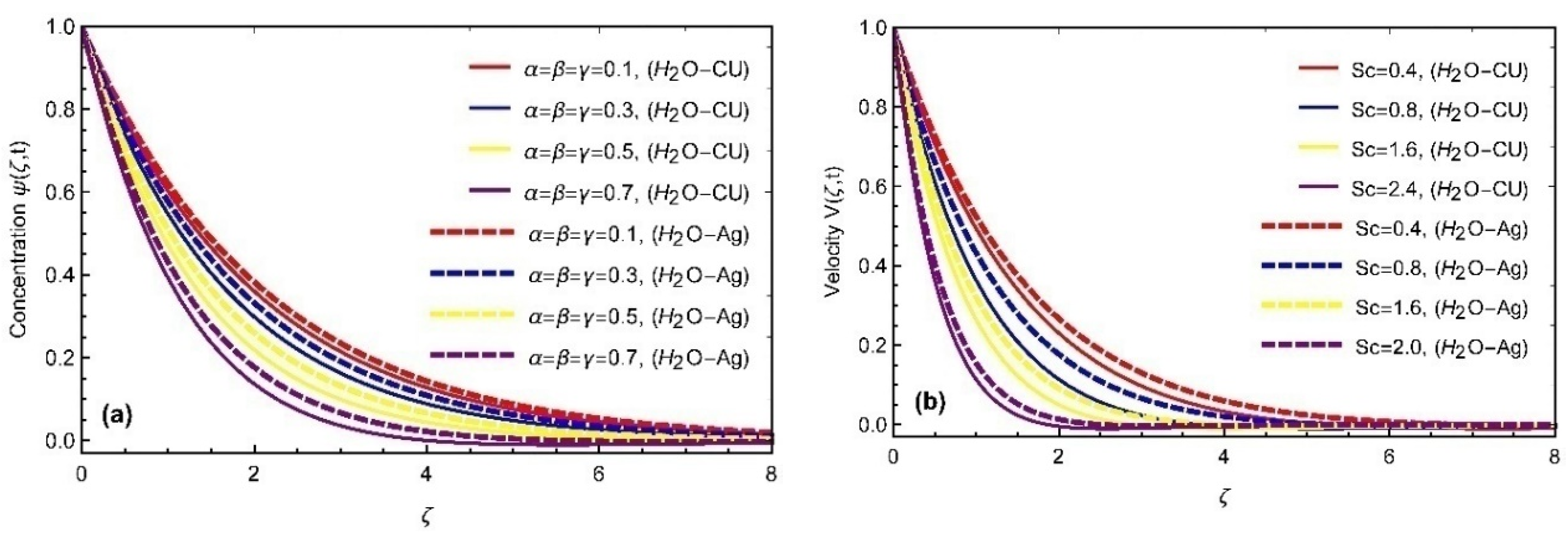
• The concentration field also declined with the Schmidt number and the fractional constraints variation.
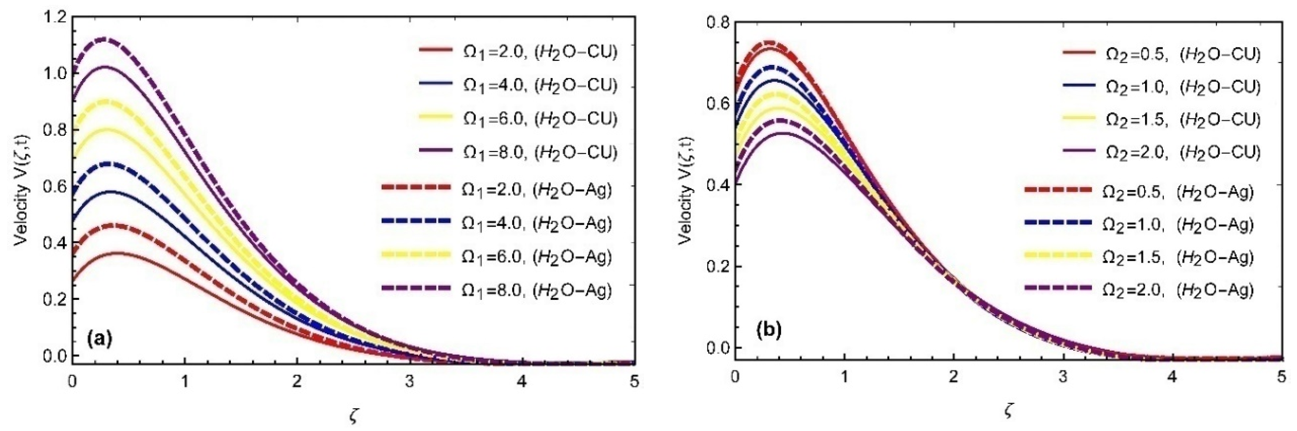
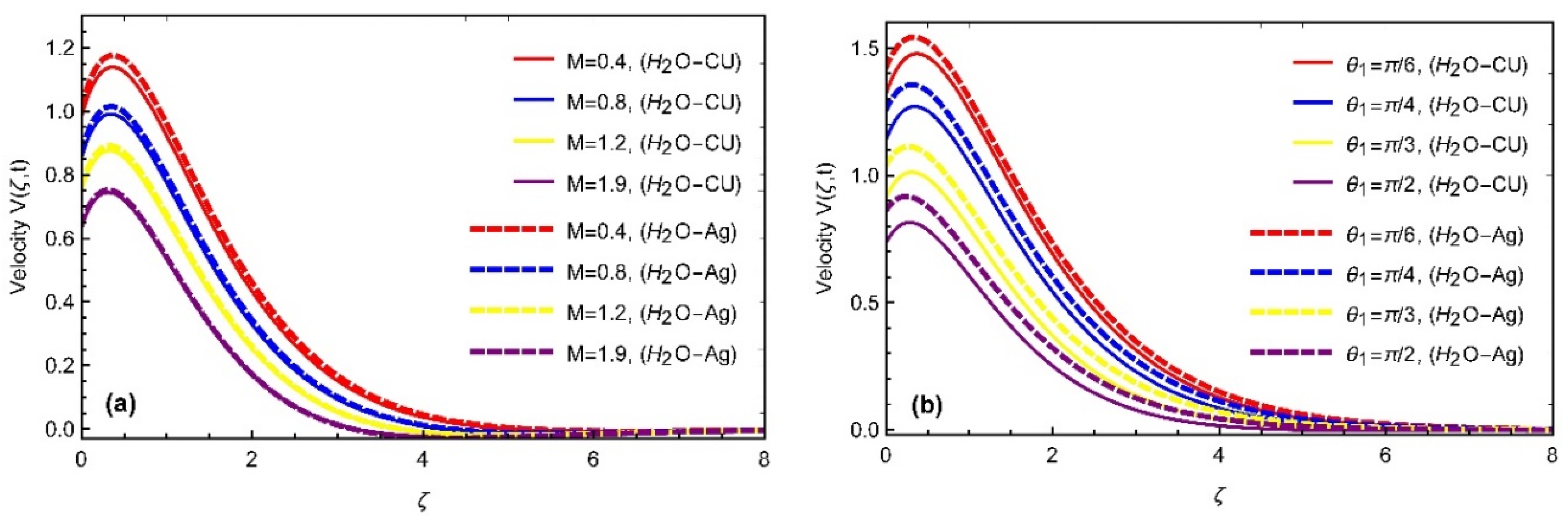
• The velocity delays by changing fractional parameters values as well as $Pr,Sc,M, \mathrm{and} K$.
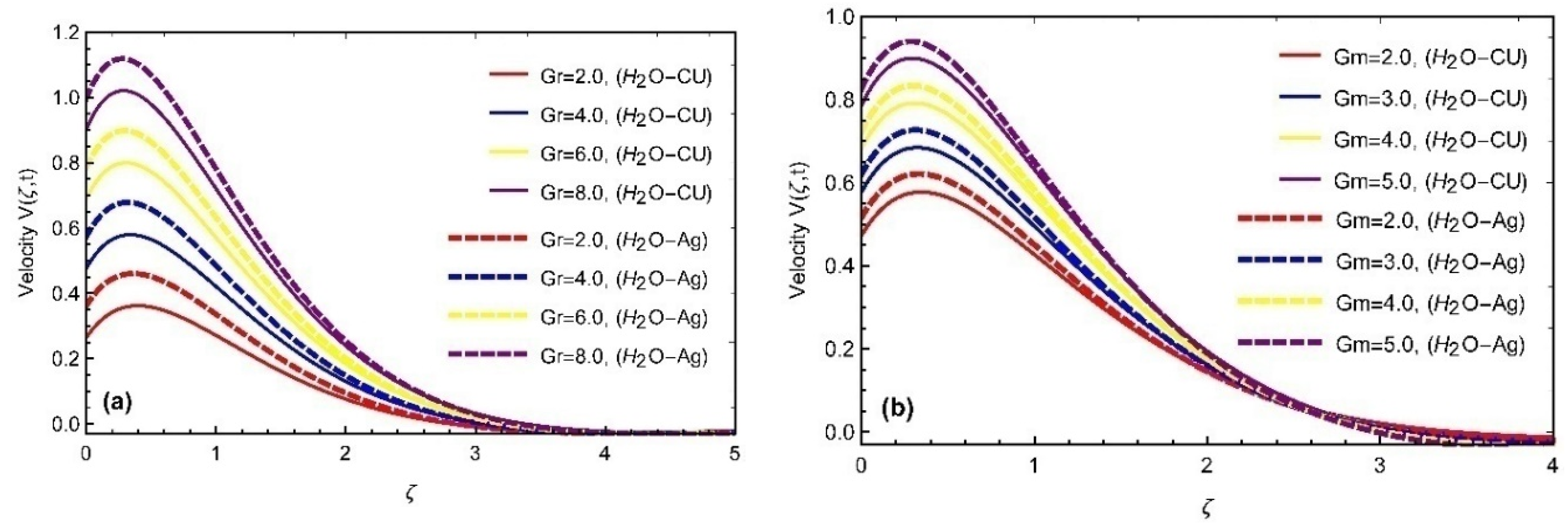
• The momentum profile increase by augmenting the amount of mass and heat Grashof number $Gm,Gr$ due to the buoyancy effect.
• It is examined that the impact of both parameters ${\mathsf{\Omega }}_1,{\mathsf{\Omega }}_2$ are opposite to the momentum field.
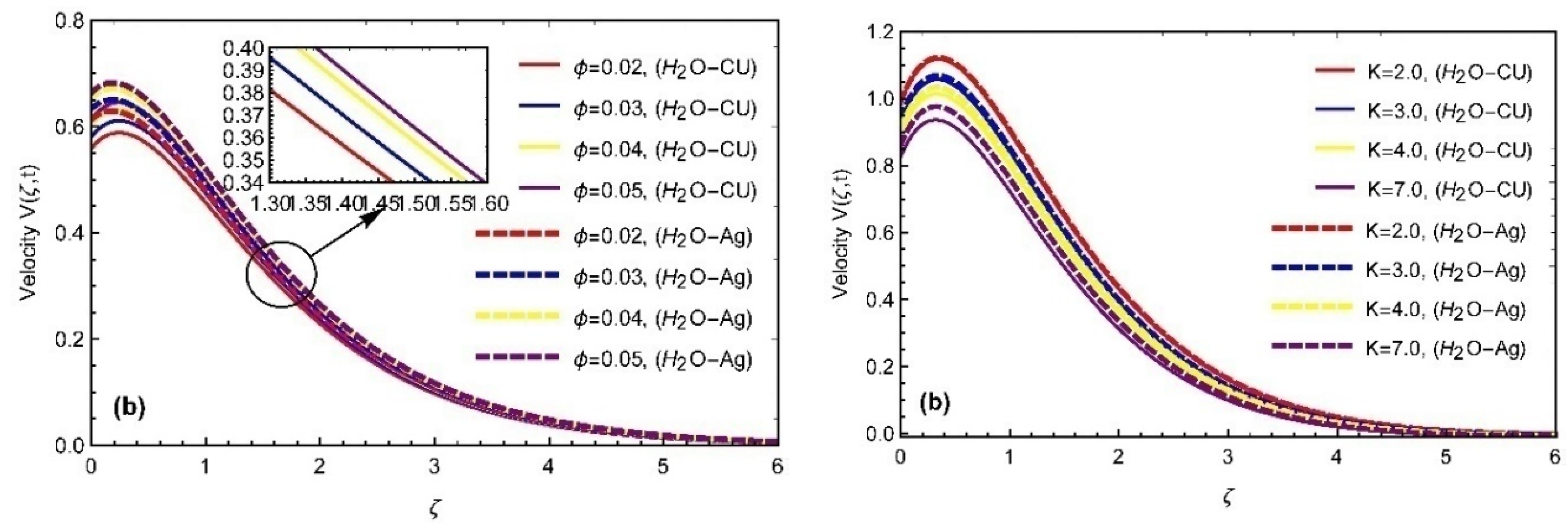
• For magnetic and permeability constraints, the viscosity of the hybrid nanofluid losses causes the fluid to slow the motion.
• The thermal and momentum profiles are more progressive for silver $\left(Ag\right)$ nanoparticles as compared to copper $\left(Cu\right)$ based nanofluid.
• The interchanging of both curves of the numerical scheme and the obtained results of Riaz et al. [42] validate this study’s solutions.

In order to suggest a future extension of the problem examined in this paper, we idolize the following recommendations based on techniques, expansions, geometries, and analysis. The present problem may be analyzed on a horizontal plate of constant length along with the linear velocity. The same problem can also be examined by exploiting Keller Box scheme.

References

1. Ghosh, A.; Sana, P. On hydromagnetic flow of an Oldroyd-B fluid near a pulsating plate. Acta Astronaut. 2009, 64, 272–280. [Google Scholar] [CrossRef]
2. Zaman, H.; Ahmad, Z.; Ayub, M. A Note on the Unsteady Incompressible MHD Fluid Flow with Slip Conditions and Porous Walls. Int. Sch. Res. Not. 2013, 2013, 705296. [Google Scholar] [CrossRef] [Green Version]
3. Nadeem, S.; Mehmood, R.; Akbar, N.S. Non-orthogonal stagnation point flow of a nano non-Newtonian fluid towards a stretching surface with heat transfer. Int. J. Heat Mass Transf. 2012, 57, 679–689. [Google Scholar] [CrossRef]
4. Tiwana, M.H.; Mann, A.B.; Rizwan, M.; Maqbool, K.; Javeed, S.; Raza, S.; Khan, M.S. Unsteady Magnetohydrodynamic Convective Fluid Flow of Oldroyd-B Model Considering Ramped Wall Temperature and Ramped Wall Velocity. Mathematics 2019, 7, 676. [Google Scholar] [CrossRef] [Green Version]
5. Zhao, J.; Zheng, L.; Zhang, X.; Liu, F. Convection heat and mass transfer of fractional MHD Maxwell fluid in a porous medium with Soret and Dufour effects. Int. J. Heat Mass Transf. 2016, 103, 203–210. [Google Scholar] [CrossRef]
6. Hayat, T.; Siddiqui, A.; Asghar, S. Some simple flows of an Oldroyd-B fluid. Int. J. Eng. Sci. 2001, 39, 135–147. [Google Scholar] [CrossRef]
7. Hayat, T.; Khan, M.; Ayub, M. Exact solutions of flow problems of an Oldroyd-B fluid. Appl. Math. Comput. 2004, 151, 105–119. [Google Scholar] [CrossRef]
8. Siddiqui, A.; Haroon, T.; Zahid, M.; Shahzad, A. Effect of slip condition on unsteady flows of an Oldroyd-B fluid between parallel plates. World Appl. Sci. J. 2011, 13, 2282–2287. [Google Scholar]
9. Riaz, M.; Imran, M.; Shabbir, K. Analytic solutions of Oldroyd-B fluid with fractional derivatives in a circular duct that applies a constant couple. Alex. Eng. J. 2016, 55, 3267–3275. [Google Scholar] [CrossRef] [Green Version]
10. Riaz, M.B.; Siddique, I.; Saeed, S.T.; Atangana, A. MHD Oldroyd-B Fluid with Slip Condition in view of Local and Nonlocal Kernels. J. Appl. Comput. Mech. 2020, 7, 116–127. [Google Scholar] [CrossRef]
11. Baranovskii, E.S.; Artemov, M. Global Existence Results for Oldroyd Fluids with Wall Slip. Acta Appl. Math. 2016, 147, 197–210. [Google Scholar] [CrossRef]
12. Le Roux, C. On Flows of Viscoelastic Fluids of Oldroyd Type with Wall Slip. J. Math. Fluid Mech. 2013, 16, 335–350. [Google Scholar] [CrossRef] [Green Version]
13. Iftikhar, N.; Saeed, S.T.; Riaz, M.B. Fractional study on heat and mass transfer of MHD Oldroyd-B fluid with ramped velocity and temperature. Comput. Methods Differ. Eq. 2021, 10, 372–395. [Google Scholar] [CrossRef]
14. Anwar, T.; Kumam, P.; Thounthong, P.; Muhammad, S.; Duraihem, F.Z. Generalized thermal investigation of unsteady MHD flow of Oldroyd-B fluid with slip effects and Newtonian heating; a Caputo-Fabrizio fractional model. Alex. Eng. J. 2021, 61, 2188–2202. [Google Scholar] [CrossRef]
15. Mburu, Z.M.; Nayak, M.K.; Mondal, S.; Sibanda, P. Impact of irreversibility ratio and entropy generation on three-dimensional Oldroyd-B fluid flow with relaxation–retardation viscous dissipation. Indian J. Phys. 2021, 96, 151–167. [Google Scholar] [CrossRef]
16. Wang, Y.; Kumar, R.N.; Gouadria, S.; Helmi, M.M.; Gowda, R.P.; El-Zahar, E.R.; Prasannakumara, B.; Khan, M.I. A three-dimensional flow of an Oldroyd-B liquid with magnetic field and radiation effects: An application of thermophoretic particle deposition. Int. Commun. Heat Mass Transf. 2022, 134, 106007. [Google Scholar] [CrossRef]
17. Caputo, M.; Fabrizio, M. A new definition of fractional derivative without singular kernel. Prog. Fract. Differ. Appl. 2015, 1, 73–85. [Google Scholar]
18. Atangana, A.; Baleanu, D. New fractional derivatives with nonlocal and non-singular kernel: Theory and application to heat transfer model. arXiv 2016, arXiv:1602.03408. [Google Scholar] [CrossRef] [Green Version]
19. Prabhakar, T.R. A singular integral equation with a generalized Mittag Leffler function in the kernel. Yokohama Math. J. 1971, 19, 7–15. [Google Scholar]
20. Kilbas, A.A.; Saigo, M.; Saxena, R.K. Generalized mittag-leffler function and generalized fractional calculus operators. Integral Transform. Spéc. Funct. 2004, 15, 31–49. [Google Scholar] [CrossRef]
21. Garra, R.; Gorenflo, R.; Polito, F.; Tomovski, Ž. Hilfer–Prabhakar derivatives and some applications. Appl. Math. Comput. 2014, 242, 576–589. [Google Scholar] [CrossRef] [Green Version]
22. Fernandez, A.; Baleanu, D. Classes of operators in fractional calculus: A case study. Math. Methods Appl. Sci. 2021, 44, 9143–9162. [Google Scholar] [CrossRef]
23. Giusti, A.; Colombaro, I.; Garra, R.; Garrappa, R.; Polito, F.; Popolizio, M.; Mainardi, F. A Practical Guide to Prabhakar Fractional Calculus. Fract. Calc. Appl. Anal. 2020, 23, 9–54. [Google Scholar] [CrossRef] [Green Version]
24. Alharbi, K.A.M.; Mansir, I.B.; Al-Khaled, K.; Khan, M.I.; Raza, A.; Khan, S.U.; Ayadi, M.; Malik, M.Y. Heat transfer enhancement for slip flow of single-walled and multi-walled carbon nanotubes due to linear inclined surface by using modified Prabhakar fractional approach. Arch. Appl. Mech. 2022, 1–11. [Google Scholar] [CrossRef]
25. Wang, Y.; Mansir, I.B.; Al-Khaled, K.; Raza, A.; Khan, S.U.; Khan, M.I.; Ahmed, A.E.-S. Thermal outcomes for blood-based carbon nanotubes (SWCNT and MWCNTs) with Newtonian heating by using new Prabhakar fractional derivative simulations. Case Stud. Therm. Eng. 2022, 32, 101904. [Google Scholar] [CrossRef]
26. Jie, Z.; Khan, M.I.; Al-Khaled, K.; El-Zahar, E.R.; Acharya, N.; Raza, A.; Khan, S.U.; Xia, W.-F.; Tao, N.-X. Thermal transport model for Brinkman type nanofluid containing carbon nanotubes with sinusoidal oscillations conditions: A fractional derivative concept. Waves Random Complex Media 2022, 1–20. [Google Scholar] [CrossRef]
27. Raza, A.; Thumma, T.; Al-Khaled, K.; Khan, S.U.; Ghachem, K.; Alhadri, M.; Kolsi, L. Prabhakar fractional model for viscous transient fluid with heat and mass transfer and Newtonian heating applications. Waves Random Complex Media 2022, 1–17. [Google Scholar] [CrossRef]
28. Wang, Y.; Raza, A.; Khan, S.U.; Ijaz Khan, M.; Ayadi, M.; El-Shorbagy, M.A.; Alshehri, N.A.; Wang, F.; Malik, M.Y. Prabhakar fractional simulations for hybrid nanofluid with aluminum oxide, titanium oxide and copper nanoparticles along with blood base fluid. Waves Random Complex Media 2022, 1–20. [Google Scholar] [CrossRef]
29. Ying-Qing, S.; Ali, R.; Kamel, A.-K.; Saadia, F.; Qiu-Hong, S.; Malik, M.Y. Significances of exponential heating and Darcy’s law for second grade fluid flow over oscillating plate by using Atangana-Baleanu fractional derivatives. Case Stud. Therm. Eng. 2021, 27, 101266. [Google Scholar]
30. Fernandez, A.; Özarslan, M.A.; Baleanu, D. On fractional calculus with general analytic kernels. Appl. Math. Comput. 2019, 354, 248–265. [Google Scholar] [CrossRef] [Green Version]
31. Giusti, A. General fractional calculus and Prabhakar’s theory. Commun. Nonlinear Sci. Numer. Simul. 2020, 83, 105114. [Google Scholar] [CrossRef] [Green Version]
32. Raza, A.; Ghaffari, A.; Khan, S.U.; Haq, A.U.; Khan, M.I. Non-singular fractional computations for the radiative heat and mass transfer phenomenon subject to mixed convection and slip boundary effects. Chaos, Solitons Fractals 2021, 155, 111708. [Google Scholar] [CrossRef]
33. Raza, A.; Al-Khaled, K.; Khan, M.I.; Khan, S.U.; Farid, S.; Haq, A.U.; Muhammad, T. Natural convection flow of radiative maxwell fluid with Newtonian heating and slip effects: Fractional derivatives simulations. Case Stud. Therm. Eng. 2021, 28, 101501. [Google Scholar] [CrossRef]
34. Riaz, M.B.; Atangana, A.; Saeed, S.T. MHD-free Convection Flow Over a Vertical Plate with Ramped Wall Temperature and Chemical Reaction in View of Nonsingular Kernel. Fract. Order Anal. Theory Methods Appl. 2020, 253–282. [Google Scholar] [CrossRef]
35. Riaz, M.B.; Saeed, S.T. Comprehensive analysis of integer-order, Caputo-Fabrizio (CF) and Atangana-Baleanu (ABC) fractional time derivative for MHD Oldroyd-B fluid with slip effect and time dependent boundary condition. Discret. Contin. Dyn. Syst.-S 2021, 14, 3719. [Google Scholar] [CrossRef]
36. Asghar, S.; Parveen, S.; Hanif, S.; Siddiqui, A.; Hayat, T. Hall effects on the unsteady hydromagnetic flows of an Oldroyd-B fluid. Int. J. Eng. Sci. 2003, 41, 609–619. [Google Scholar] [CrossRef]
37. Anwar, T.; Khan, I.; Kumam, P.; Watthayu, W. Impacts of Thermal Radiation and Heat Consumption/Generation on Unsteady MHD Convection Flow of an Oldroyd-B Fluid with Ramped Velocity and Temperature in a Generalized Darcy Medium. Mathematics 2020, 8, 130. [Google Scholar] [CrossRef] [Green Version]
38. Raza, A.; Khan, S.U.; Khan, M.I.; Farid, S.; Muhammad, T.; Galal, A.M. Fractional order simulations for the thermal determination of graphene oxide (GO) and molybdenum disulphide (MoS2) nanoparticles with slip effects. Case Stud. Therm. Eng. 2021, 28, 101453. [Google Scholar] [CrossRef]
39. Raza, A.; Khan, I.; Farid, S.; My, C.A.; Khan, A.; Alotaibi, H. Non-singular fractional approach for natural convection nanofluid with Damped thermal analysis and radiation. Case Stud. Therm. Eng. 2021, 28, 101373. [Google Scholar] [CrossRef]
40. Guo, B.; Raza, A.; Al-Khaled, K.; Khan, S.U.; Farid, S.; Wang, Y.; Khan, M.I.; Malik, M.; Saleem, S. Fractional-order simulations for heat and mass transfer analysis confined by elliptic inclined plate with slip effects: A comparative fractional analysis. Case Stud. Therm. Eng. 2021, 28, 101359. [Google Scholar] [CrossRef]
41. Ghalib, M.M.; Zafar, A.A.; Farman, M.; Akgül, A.; Ahmad, M.O.; Ahmad, A. Unsteady MHD flow of Maxwell fluid with Caputo–Fabrizio non-integer derivative model having slip/non-slip fluid flow and Newtonian heating at the boundary. Indian J. Phys. 2021, 96, 127–136. [Google Scholar] [CrossRef]
42. Riaz, M.B.; Awrejcewicz, J.; Rehman, A.-U.; Akgül, A. Thermophysical Investigation of Oldroyd-B Fluid with Functional Effects of Permeability: Memory Effect Study Using Non-Singular Kernel Derivative Approach. Fractal Fract. 2021, 5, 124. [Google Scholar] [CrossRef]
Figure 1. Flow geometry.
Fractalfract 06 00357 g001
Figure 2. Temperature for fractional parameters with P r = 5.4 ,   φ = 0.02 at (a) t = 0.5 , (b) t = 1.5 , (c) t = 0.5 and (d) t = 1.5 .
Fractalfract 06 00357 g002
Figure 3. Temperature profiles for (a) α ,   β ,   γ and (b) P r with φ = 0.02 ,   t = 1.0 .
Fractalfract 06 00357 g003
Figure 4. Concentration profiles for (a) α ,   β ,   γ and (b) S c with φ = 0.02 ,   t = 1.0 .
Fractalfract 06 00357 g004
Figure 5. Momentum fields for (a) α ,   β ,   γ and (b) α ,   β ,   γ   and   h with α = β = γ = 0.6 ,   P r = 6.0 ,   S c = 1.6 ,   G r = 6.2 ,   G m = 4.3 ,   h = 0.5 ,   K = 3.2 ,   M = 1.2 ,   θ 1 = θ 2 = π 3 ,   φ = 0.02 ,   t = 1.0 .
Fractalfract 06 00357 g005
Figure 6. Momentum fields for (a) Ω 1   ( h i g h e r   v a l u e s ) and (b) Ω 1   ( l o w e r   v a l u e s ) with α = β = γ = 0.6 ,   P r = 6.0 ,   S c = 1.6 ,   G r = 6.2 ,   G m = 4.3 ,   h = 0.5 ,   K = 3.2 ,   M = 1.2 ,   θ 1 = θ 2 = π 3 ,   φ = 0.02 ,   t = 1.0 .
Fractalfract 06 00357 g006
Figure 7. Momentum fields for (a) G r and (b) G m with α = β = γ = 0.6 ,   P r = 6.0 ,   S c = 1.6 ,   h = 0.5 ,   K = 3.2 ,   G r = 6.2 ,   G m = 4.3 ,   M = 1.2 ,   θ 1 = θ 2 = π 3 ,   φ = 0.02 ,   t = 1.0 .
Fractalfract 06 00357 g007
Figure 8. Momentum fields for (a) P r and (b) S c with α = β = γ = 0.6 ,   P r = 6.0 ,   S c = 1.6 ,   G r = 6.2 ,   G m = 4.3 ,   h = 0.5 ,   K = 3.2 ,   M = 1.2 ,   θ 1 = θ 2 = π 3 ,   φ = 0.02 ,   t = 1.0 .
Fractalfract 06 00357 g008
Figure 9. Momentum fields for (a) φ and (b) K with α = β = γ = 0.6 ,   P r = 6.0 ,   S c = 1.6 ,   G r = 6.2 ,   G m = 4.3 ,   h = 0.5 ,   K = 3.2 ,   M = 1.2 ,   θ 1 = θ 2 = π 3 ,   φ = 0.02 ,   t = 1.0 .
Fractalfract 06 00357 g009
Figure 10. Momentum fields for (a) M and (b) θ 1 with α = β = γ = 0.6 ,   P r = 6.0 ,   S c = 1.6 ,   G r = 6.2 ,   G m = 4.3 ,   h = 0.5 ,   K = 3.2 ,   M = 1.2 ,   θ 1 = θ 2 = π 3 ,   φ = 0.02 ,   t = 1.0 .
Fractalfract 06 00357 g010