Optimal Majority Rule in Referenda


1
Department of Theory, Party School of Haimen Committee of CPC (Haimen Administration Institute), Haimen 226100, China
2
1455 Boulevard de Maisonneuve Ouest, Department of Economics, Concordia University, Montreal, QC H3G 1M8, Canada
3
CIRANO, Montreal, QC H3A 2M8, Canada
4
CIREQ, Montreal, QC H3T 1N8, Canada
*
Author to whom correspondence should be addressed.
Games 2019, 10(2), 25; https://0-doi-org.brum.beds.ac.uk/10.3390/g10020025
Submission received: 1 May 2019
/
Revised: 27 May 2019
/
Accepted: 29 May 2019
/
Published: 3 June 2019
(This article belongs to the Special Issue Political Economy, Social Choice and Game Theory)
Abstract
:Adopting the group turnout model of Herrera and Mattozzi, J. Eur. Econ. Assoc. 2010, 8, 838–871, we investigate direct democracy with supermajority rule and different preference intensities for two sides of a referendum: Reform versus status quo. Two parties spend money and effort to mobilize their voters. We characterize the set of pure strategy Nash equilibria. We investigate the optimal majority rule that maximizes voters’ welfare. Using an example, we show that the relationship between the optimal majority rule and the preference intensity is not monotonic—the optimal majority rule is initially decreasing and then increasing in the preference intensity of the status quo side. We also show that when the preference intensity of the status quo side is higher, the easiness to mobilize voters on the status quo side is lower, or the payoff that the reform party receives is higher, the optimal majority rule is more likely to be supermajority.
1. Introduction
A referendum is a mechanism through which all citizens collectively make a decision on major issues. Recent examples include the British vote on EU membership in 2016 (commonly known as “Brexit”) and the Scottish vote on UK membership in 2014. Since the Second World War, most of the world’s countries are moving towards a greater use of referenda and paying more attention to designs and implementation of referenda. Referenda have become an established mechanism for decision-making in democratic systems.
Despite its wide use, the adoption of referenda as a decision mechanism is often controversial. Outcomes of referenda are sometimes far from voters’ expectations. Two recent instances are the shock Brexit vote and the failure of the Italian constitutional reforms. Given the significant consequences of these referenda, if not properly designed and managed, they have the potential of causing division and instability in society.
Take the Brexit referendum as an example. In 2016, the United Kingdom held a referendum on June 23 to decide whether the UK should leave or remain in the European Union. The outcome was that 17.4 million people voted to leave the EU while 16.1 million people voted to stay. Leave won by 51.9% to 48.1%. The referendum turnout was 72.21%, with more than 30 million people voting. Leave scored a narrow victory over Remain. On the day after the referendum, Prime Minister David Cameron announced his resignation. More than 4 million people signed a petition calling for a second EU referendum to be held. The petition reads: “we the undersigned call upon HM Government to implement a rule that if the remain or leave vote is less than 60% based a turnout less than 75% there should be another referendum.” However, the British government formally rejected the petition on 9 July 2016. The economist Kenneth Rogoff [1] of Harvard University considers the Brexit vote as a democratic failure: “The real lunacy of the United Kingdom’s vote to leave the European Union was not that British leaders dared to ask their populace to weigh the benefits of membership against the immigration pressures it presents. Rather, it was the absurdly low bar for exit, requiring only a simple majority. Given voter turnout of 70%, this meant that the leave campaign won with only 36% of eligible voters backing it.” As of this writing, the UK parliament has yet to pass any bill that would ensure an orderly Brexit.
Referenda often adopt the simple majority rule, as did the Brexit referendum. Qvortrup [2] provides a list of majority provisions in established Western Democracies. See Table 1 for a list of the threshold requirements for referenda held in established Western democracies. The aforementioned commentary from Kenneth Rogoff illustrates a potent critique of the simple majority rule, namely, changes that have major consequences should be required to garner strong support by clearing a supermajority.
Another frequently cited critique of the simple majority rule is that close (50-50) outcomes tend to be controversial and destabilizing per se. Qvortrup [2] argues that “A close result threatens the legitimacy of the outcome” (p.174), and quotes former Canadian Foreign Minister Stephane Dion arguing that “you don’t break a country with support of 50% plus one” (p.166). The experience from before and after the Brexit referendum arguably provides some evidence in favour of this viewpoint. In Table 2, there are a handful of examples of referenda that were decided by a whisker.
The above two critiques make it worthwhile to consider alternatives to the simple majority rule. In practice, supermajority provisions led to the defeat of the devolution proposal of Scotland in the UK and to the defeat of several laws in Italy. Also, the Treaty of Lisbon has adopted a double majority system for the EU Council; the system requires a majority of votes according to two separate criteria.
The discussion about majority rules is connected to the true meaning of democracy. The famous commentator on American democracy, Alexis de Tocqueville, wrote extensively about the tyranny of the majority in his book, “Democracy in America.” This is when the majority rule—the basis of democracy—ends up perverting democracy by forcing injustice on the minority. For example, Proposition 8, a California ballot proposition, was passed in 2008 to amend the California constitution and ban gay marriages. The ban was later ruled unconstitutional by the Federal courts because it was viewed as removing rights from a disfavored class but with no rational basis. In the context of financing public good through taxation, Wicksell [3] argues in favour of unanimity-voting rule based on the benefit principle to taxation, as unanimity would guarantee that all individuals receive benefits commensurate to their tax cost from any public good. Buchanan and Tullock [4] argue that supermajorities could mitigate the “tyranny of the majority.” We should point out Rae [5] argues that simple majority is the only rule that minimizes the ex ante expected cost of being a part of the minority.
In this paper, we analyze the effect of the optimal majority rule in referenda. We adopt the group turnout model developed by Herrera and Mattozzi [6] based on Snyder [7] and Shachar and Nalebuff [8], where two opposing parties spend effort to mobilize their supporters to the polls, while facing aggregate uncertainty on the voters’ preferences. Herrera and Mattozzi [6] mainly analyze how a participation/quorum requirement affects the voting outcomes. We add to their model new parameters in referenda: A general majority rule, different preference intensities of the two sides (reform versus status quo), and different levels of easiness to mobilize each side. In fact, in the working paper version of their published work, Herrera and Mattozzi [9] do consider heterogeneous preference intensities for the two sides, but our main contribution is our analysis of the optimal majority rule.
Under relatively general assumptions, we characterize pure-strategy Nash equilibria between the parties and prove that they always exist. We show that Nash equilibrium is unique if both parties have the same preference intensity and voters of both sides have the same benefit function from voting. In addition, we analyze an example where there exists a unique pure-strategy Nash equilibrium by giving a specific benefit function to the voter who supports that party’s policy. We then perform a welfare analysis and characterize the optimal majority rule for the referendum.
We then adopt a more specialized setup, so as to conduct comparative statics analyses. We first investigate the relationship between the optimal majority rule and the preference intensity of the status quo side. Somewhat surprisingly, the relationship is not monotonic—the optimal majority rule is initially decreasing and then increasing in the preference intensity of the status quo side.
We then investigate the relationship between the optimal majority rule and the payoffs that the parties receive. The optimal majority rule decreases as the importance of the referendum increases if the preference intensity of the status quo side is less than a critical value, which is determined by the relative easiness to mobilize the reform side versus the status quo side. Conversely, the optimal majority rule increases as the importance of the referendum increases. Also, at this critical value, the optimal majority rule is independent of the importance of the referendum.
We investigate when the optimal majority rule is likely to be supermajority. We show that the optimal majority rule is more likely to be supermajority when the status quo side is more difficult to mobilize, when the preference intensity of the status quo side is higher, when the reform side is easier to mobilize than the status quo side, or when the payoff that the reform party receives is higher.
Related Literature
The most closely related work is that by Herrera and Mattozzi [6] who, as mentioned above, investigate the effect of quorum requirement on the outcome of referenda. They identify a “quorum paradox,” namely, the fact that the expected equilibrium turnout will never meet the imposed quorum requirement. They also show that a quorum requirement is not necessarily pro-status quo and is not equivalent to a supermajority threshold for reform. In contrast, we investigate the optimal majority rule by maximizing voters’ welfare. We adopt their theoretical model, which is in turn derived from Shachar and Nalebuff’s [8] group turnout model, who show that participation rate and political parties’ efforts are a positive function of predicted closeness and a negative function of the voting population size.
Our optimization approach is similar in spirit to that of Osborne and Turner [10], who study whether a referendum or a cost–benefit analysis leads to higher welfare, and show that the outcome of a cost–benefit analysis is superior when individuals have diverse preferences but similar information, whereas the outcome of a referendum is superior when individuals have similar preferences but different degrees of uncertainty. Taking the behavioral approach but not in the context of referenda, Attanasi, Corazzini, and Passarelli [11] investigate the optimality of supermajority and show that an individual prefers a higher majority threshold when she is more risk averse, less powerful, or less optimistic about how others will vote. Dal Bo [12] suggests that appropriate supermajority requirements induce the right conservative bias, solving possible time inconsistency problems in policy making. Finally, Messner and Polborn [13] endogenize the majority rule for a collective decision on a new investment and show that relative to young voters, older voters are more conservative and prefer higher thresholds because they pay more taxes and have less opportunity to benefit from fiscal returns of some investment expenditure and later payoff.
The easiness to mobilize is a parameter of interest our model. The intuition “High turnout is a result of increased effort that parties exert” is supported by the empirical work of Kramer [14] and Wielhouwer and Lockerbie [15], who show that respondents who were contacted by the parties are more likely to participate. In recent work, Spenkuch and Toniatti [16] find no evidence that advertising has an impact on overall turnout. In the aggregate, the mobilizing and demobilizing effects of political ads tend to cancel out. By contrast, they present evidence of a positive and economically meaningful impact of advertising on candidates’ vote shares.
We also want to point out the study of preference-aggregation institutions that improve upon simple plurality is a broader question, as reflected in writings in political philosophy and institutional economics. We will not provide an exhaustive discussion here but point the interested reader to a few classics.1 Bentley [17] argues in favour of interest group plurality, observing that it accounts for intensity of preferences. However, Olson [18] points out that the formation of interest groups may be a distortion of population preferences. Cost–benefit analysis is another potential approach, but it requires the experts to have relatively precise information about preferences of the public. Coasian bargaining (Coase [19]) between individuals/groups is a potential solution, when transfers are feasible. In recent work, Munger [20] relates and compares these different institutions.
We now preview the rest of the paper. In Section 2, we present and analyze a model for referenda. We focus on pure-strategy Nash equilibrium, and the voters’ welfare optimization problem. We also analyze the specific optimal majority rule and supermajority requirement through an example. We conclude in Section 3, where we summarize results of this paper, discuss their policy implications, and suggest further research. The Appendix A collects detailed proofs of results in the main text.
2. Model
2.1. Model Setup
We study a variation of the model studied by Herrera and Mattozzi [6]. The setup is identical, but we introduce a general majority rule requirement for approving the reform.
Consider a direct democracy consisting of individuals legally eligible to vote in a society. Each individual can only choose between two alternatives: r (reform) and s (status quo). Government selects a majority rule , defining the fraction of voters that must approve a policy proposed to replace the status quo. The unanimity rule, for example, is defined by , while is the simple majority rule.
There are two exogenously given parties supporting policies r and s, and a continuum of voters of measure 1, of which a proportion supports policy r, and the remaining supports policy s. Assume that is a random variable with uniform distribution. One should interpret as a reflection of the aggregate uncertainty about the proportion of voters supporting each alternative. Each voter has a personal cost of voting that is also drawn from a uniform distribution.
Parties decide simultaneously the amount of campaign funds to spend (equivalently, the amount of effort to exert) to mobilize voters in order to win the referendum. Let be the payoff that the reform party receives when reform passes and be the payoff that the status quo party receives when reform fails. Thus, can be viewed as a measure of the importance of the referendum and is the preference intensity of the status quo side versus the reform side. We use to represent both the intensity of preferences of the party and the voters, assuming the party and their constituents have aligned preferences. The parties’ objective functions are
where P is the (endogenous) probability that alternative r is selected and are the spending of parties’ r and s, respectively.
Voters decide whether to vote in the referendum or not depending on the benefit they receive from the party and their cost of voting. To streamline the model and to follow Herrera and Mattozzi’s [6] setup, we assume that each voter faces the same cost of voting, . On the other hand, we assume that voters receive a benefit from voting for their preferred policy that is increasing and strictly concave in parties’ mobilization efforts. In particular, if a party spends x, the benefit to a voter who supports that party’s policy is is continuous, twice differentiable for , strictly increasing, strictly concave, and satisfies the properties
This specification is equivalent to having parties’ expenditures affect individual cost of voting.2 In particular, the mobilization functions and potentially reflect the intensity of the voters’ preferences, as well other factors that may impact mobilization, which may include the ages of voters on each side, whether one side of the voters are predominantly minority, how well the infrastructures of political organization are, etc.3 Note that we do not explicitly include the intensity of preference parameter in these mobilization functions, to maintain the flexibility of these functions. As Olson [18] rightfully points out, the parties’ mobilization effort may not actually reflect the underlying intensity of preferences. Finally, for the sake of simplicity, we assume that .4
Given the above definition of the benefit from voting, for a given level of spending by the reform side, , a voter who supports policy r and has a voting cost equal to c votes for alternative r if and only if . Because this holds for fraction of the voters supporting policy r, the vote share for that policy (as a fraction of the total population) is . Likewise, the vote share for the status quo policy s is .
The reform side only wins the referendum if the actual realized proportion of voters exceeds a certain threshold. The probability that the reform policy r is selected is:
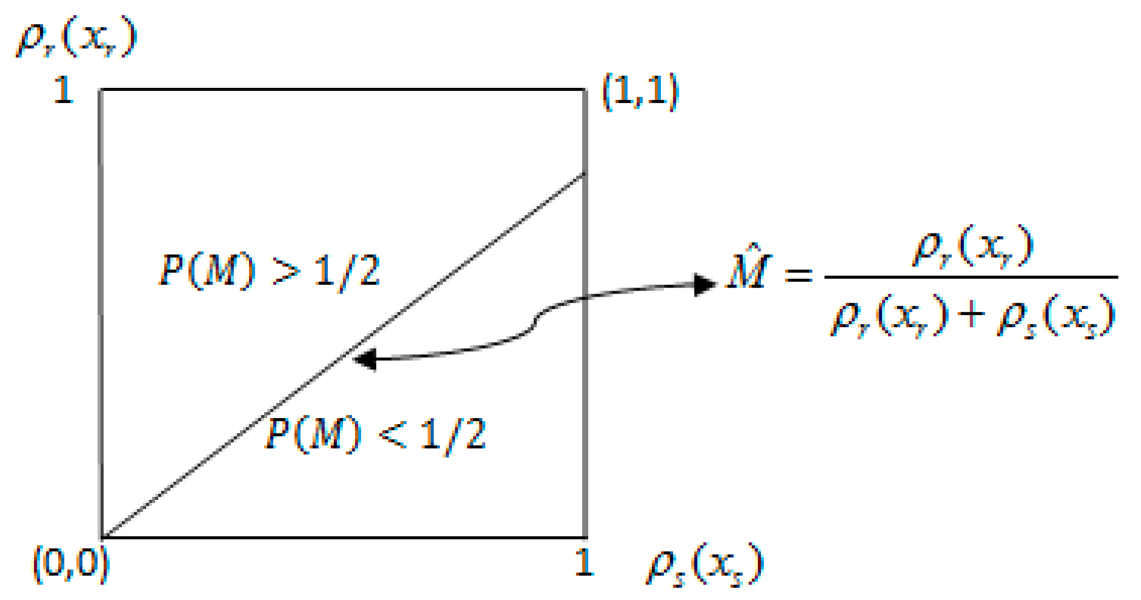
Note that P is represented as a function of and for any given , and is continuous in its arguments on the whole space . Assume that is on the vertical axis and is on the horizontal axis. Define
The equality (5) yields the line from the origin in Figure 1, which rotates counterclockwise along the origin as decreases. Also, is the region above this line; is the region below this line.
The characteristic of : The probability is decreasing in . If is equal to 1, which means there is an unanimity rule, is equal to 0. If is close to 0, is close to 1. In addition, the line in Figure 1 corresponds to , the region above the line corresponds to , and the region below the line corresponds to .
2.2. Equilibrium Characterization
Considering parties’ behavior, we start by focusing on pure-strategy Nash equilibrium.
Proposition 1 (Nash Equilibrium).
There exists a pure-strategies Nash equilibrium between parties, where the spending profileis positive, and satisfies the following two equations
where
The proof of Proposition 1 is provided in the Appendix A. There we show that and are functions of implicitly defined by
Proposition 2.
If the preference intensity of both parties is the same, and the benefit function for both groups of voters is also the same, the pure-strategies Nash equilibrium between parties exists and is unique.
Proof.
If the preference intensity of both parties is the same, and the benefit function for both groups of voters is also the same, then we have that .
Based on Equations (7) and (8), which yield
Therefore, it must be that , where solves
Because is a decreasing function in , and is the positive real numbers, an equilibrium exists, and it is unique for any B. □
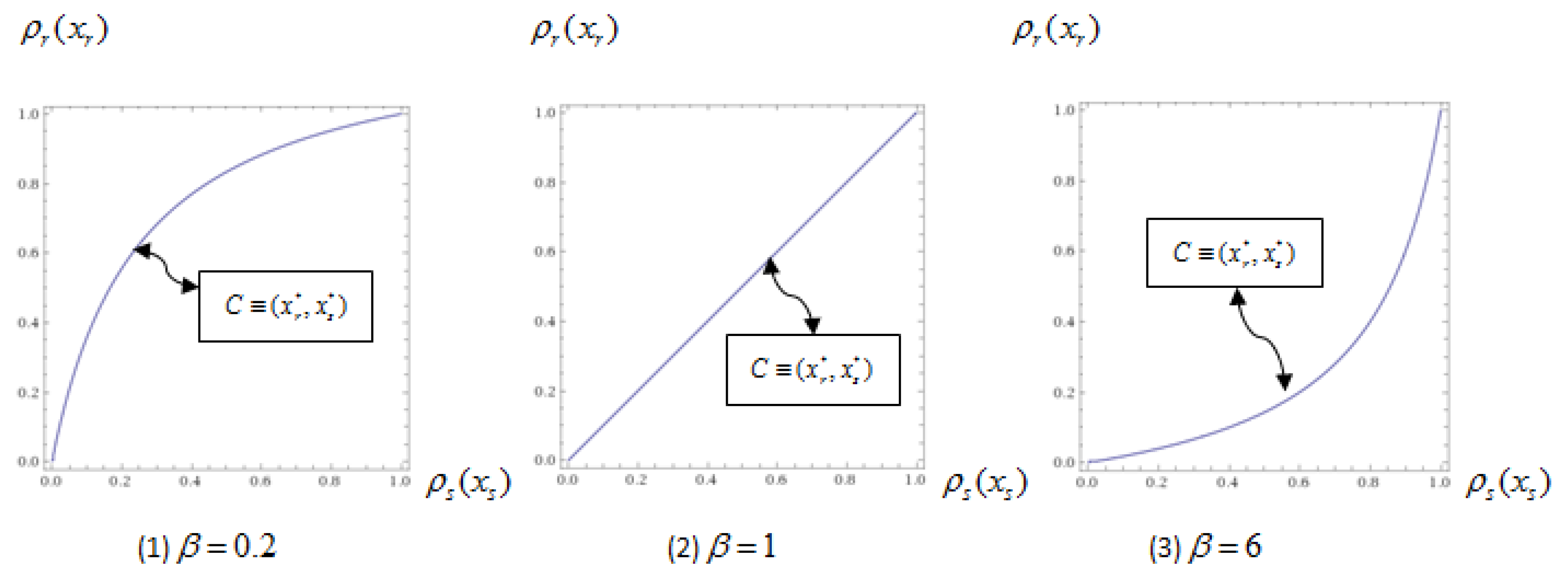
Figure 2 illustrates the pure-strategy Nash equilibrium for all values of majority rule given a specific function and specific values of . For any value of majority rule , there exists a unique corresponding pure-strategy Nash equilibrium. Typically, if the preference intensity of the status quo side is less than 1, then the best response of party r is greater than the best response of party s (); also, if , ; if , .
Proposition 3.
Given the benefit function to the voter who supports that party’s policy:, the pure-strategies Nash equilibrium between parties exists and is unique.
Proof.
Put into Equation (7), which yields
then we have
Because is a decreasing function in and because is the positive real numbers, an equilibrium exists and it is unique for any B. □
Corollary 1.
The zero spending profileis the corner pure-strategy Nash equilibrium if and only if.
The proof of Corollary 1 is provided in the Appendix A. Corollary 1 shows two extreme situations. If the majority rule close to one or zero, both the reform party and status quo party would find it optimal to not spend any funds on mobilization.
Based on (1), (2), (9), and (10), we have
- The spending of the reform party is the best response to because
- The spending of the status quo party is the best response to , because
Corollary 2.
There exists a maximum value of spending profilein the pure-strategies Nash equilibrium among all value of majority rule, where
The proof of Corollary 2 is provided in the Appendix A. In other words, among all pure-strategies Nash equilibrium, the party sides have a maximum value of spending profile for a corresponding value of majority rule . For example, there exists a point on the blue line of Figure 2 to represent the maximum value of the spending profile. Thus, there exists an upper bound of spending for parties.
In addition, is a decreasing function in , then the higher payoff of the reform party receives, the higher upper bound of spending is stipulated; and, the higher value of the preference intensity of the status quo side, the high upper bound for spending of the status quo party is stipulated.
2.3. Welfare Maximization
Now we turn to the analysis of voter welfare, which we define as the sum of the expected payoff of all voters. In other words, we adopt the ex ante utilitarian criterion in ranking outcomes.
Problem.
The maximization problem for the expected payoff of all voters
Note that represents the expected payoff of voters in favor of policy r when policy r is chosen, and represents the expected payoff of voters in favor of policy s when policy s is chosen. Here, K is a threshold point of the proportion of voters who support policy r; parameter is the preference intensity of the status quo side. Note that if , the expected payoff of voters in favor of reform is higher than the voters in favor of status quo; if , the expected payoff of voters in favor of reform is lower than the voters in favor of status quo.
Proposition 4 (Social Welfare).
The expected payoff of all voters’ reaches the maximum value if and only if the threshold value, i.e., the optimal majority rule satisfies the following equation
and the maximum value of the expected payoff of all votersis equal to.
Proof.
Solving problem
Thus, when ,
By Equation (12), we have
Then,
Note that if the preference intensity of the status quo side becomes higher, the threshold value K could become higher to obtain the higher value of the expected payoff of all voters . Specifically, if , it means there is no benefit to voters in favor of status quo, so the threshold value and a majority rule means the party in favor of status quo will not spend funds to mobilize voters. Depending on the pure-strategy Nash equilibrium, the best response of the reform party to the status quo party is also not to spend funds to mobilize voters. Thus, the pure-strategy Nash equilibrium of parties is the positive spending profile as , while the expected payoff of all voters . Please recall corollary 1.
2.4. An Example
Consider the case in which and where represents the easiness to mobilize, i.e., the larger , the easier to mobilize. As we have proved in the Proposition 1, there exists a pure-strategy Nash equilibrium between parties. In this example, the positive spending profile satisfies the following two equations
Note that we introduce parameter in the function in order to represent benefit to voters. For example, assume most young people prefer reform, while most old people prefer status quo. But younger people tend to be more urban and employed, so their voting cost is typically higher. It is therefore reasonable to assume that it is more difficult to mobilize young people than old people. Even though the party exerts the same effort, the mobilize level is different between status quo and reform. Thus, it is suitable for us to express by introducing here.
Proposition 5.
Given the benefit function to the voter who supports that party’s policy:, the pure-strategies Nash equilibrium between parties exists and is unique.
Proof.
Put into Equation (7), which yields
then we have
Because is a decreasing function in and is the positive real numbers, an equilibrium exists and it is unique for any B. □
Proposition 6 (Optimal Majority Rule).
The expected payoff of all voters reaches the maximum value if and only if the optimal majority rule
and the positive spending profile of parties
where
The proof of Proposition 6 is provided in the Appendix A. Comparative analysis for the optimal majority rule is shown as follows.
Corollary 3 (Relationship between M* and β).
There exists one critical value of
1. When
the optimal majority rule M decreases asincreases;
2. When
the optimal majority rule M increases asincreases
3. When ,
4. When ,
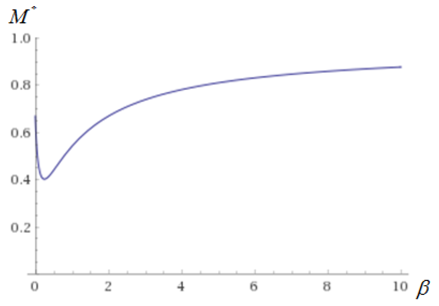
The proof of Corollary 3 is provided in the Appendix A. Note that if the preference intensity of the status quo side is close to zero, the optimal majority rule decreases from if increases a little from zero. Also, if is relatively high, the optimal majority rule increases as increases, and the value of is not more than .
It follows that if the easiness to mobilize the status quo party is relatively low, the optimal majority rule is more likely to be supermajority. In addition, there exists a minimum value of the optimal majority rule with a corresponding value of . Figure 3 illustrates the relationship between and when . The optimal majority rule decreases to the lowest point firstly, then increases as increases.
Corollary 4 (Relationship between M* and B).
There exists one critical value of
1. When, the optimal majority ruledecreases as B increases;
2. When , the optimal majority rule
which has no relation to parameter B, and equal to threshold value K.
3. When, the optimal majority ruleincreases as B increases.
4. When
5. When
The proof of Corollary 4 is provided in the Appendix A. Note that the optimal majority rule decreases from to as B increases from zero to infinite if ; increases from to as B increases from zero to infinite if ; is equal to if , and it increases as increases.
It follows that if is relatively high, the optimal majority rule is more likely to be supermajority. In addition, the optimal majority rule is not monotonic in the payoff that the reform party receives when reform passes. If , the higher optimal majority rule should be stipulated as B becomes higher.
Proposition 7 (Supermajority Requirement).
The optimal majority rule satisfies supermajority requirement if and only if
where s is a supermajority rule with s > 1/2,is the easiness to mobilize of reform party, andis the easiness to mobilize the status quo party.
The proof of Proposition 7 is provided in the Appendix A. Note that the left part of inequality is a function of the easiness to mobilize for reform and status quo, and the right part of inequality is a function of the preference intensity of the status quo side .
When ,
When ,
If ,
Thus, for supermajority requirement, this inequality also reflects the relationship between the easiness to mobilize and the payoff that the reform party receives. Note that if the easiness to mobilize the reform party is much higher than the status quo party, the optimal majority rule is more likely to be supermajority. Also, the optimal majority rule is more likely to be supermajority if the importance of the referendum is higher.
Corollary 5 (Judgment rule for supermajority requirement).
Sufficient conditions for the optimal majority rule satisfies supermajority requirement.
The proof of Corollary 5 is provided in the Appendix A.
3. Conclusions
In this paper, we characterize the optimal majority rule for referenda. To conduct our analysis, we adopt a group-turnout model of direct democracy that derives from Herrera and Mattozzi [6], who are inspired by Snyder [7] and Shachar and Nalebuff [8]. In this model, there is aggregate uncertainty about the proportion of voters who support each side.
Using comparative analysis for the optimal majority rule, we have two findings. We first investigate the relationship between the optimal majority rule and the preference intensity of the status quo side. We show that if the preference intensity of the status quo side is close to zero, the optimal majority rule is negatively related to the preference intensity of the status quo side; if the preference intensity of the status quo side is relatively high, the optimal majority rule is positively related to the preference intensity of the status quo side. For the optimal majority rule, we show that there exists a minimum value and two extreme point values, which show that the optimal majority rule is more likely to be supermajority as the easiness to mobilize the status quo party is relatively low.
We then investigate the relationship between the optimal majority rule and the payoff that the reform party receives when reform passes. We show that if the preference intensity of the status quo side is less than the ratio of easiness to mobilize two sides, the optimal majority rule is negatively related to the payoff that the reform party receives; if the preference intensity of the status quo side is greater than the ratio of easiness to mobilize two sides, the optimal majority rule is positively related to the payoff that the reform party receives; if the preference intensity of the status quo side is equal to the ratio of easiness to mobilize two sides, the optimal majority rule is a fixed value, and is positively related to the payoff that the reform party receives. The optimal majority rule is not monotonic in the payoff that the reform party receives when reform passes. Also, for the optimal majority rule, there exist two extreme point values, which show that the optimal majority rule is more likely to be supermajority as the preference intensity of the status quo side is relatively high, or the easiness to mobilize the status quo party is relatively low.
For the supermajority requirement, the inequality reflects the relationship between the easiness to mobilize and the payoff that the reform party receives. We show that the optimal majority rule is more likely to be supermajority as the easiness to mobilize the reform party is much higher than the status quo party; and the optimal majority rule is more likely to be supermajority if the importance of the referendum is higher.
We assume that both parties can rationally use the referendum funds to gain maximum benefit, and we investigate the majority rule that maximizes voters’ expected payoffs. Our analysis provides some guidance on when a supermajority rule is likely to be optimal. For example, we provide some justification for using a supermajority rule to protect minority rights. It is worth noting that our analysis abstracts from much of the realistic details and therefore should be interpreted with caution.
It is worth noting also that we take the “ex-post” approach to solving for the optimal majority rule, in that we assume the opposing sides’ preference intensities and levels of easiness to mobilize are commonly known. In contrast, Rae [5] argues that without knowing who will favour or oppose reform and how intense those preferences are, simple majority rule is welfare-maximizing. We contend that in particular classes of referenda, we are not completely ignorant about these parameters. Here, we offer two classes of cases. The first class is one where there is an intergenerational component. The outcome of the Brexit referendum would have a long-lasting impact on younger voters, much of which is negative, while it might provide short-term benefits to older voters, financial or otherwise. In the Brexit referendum, the “Leave” side campaigned heavily on the promise that the “£350m we will save” from Brexit can be used to fund the National Health System [21]. Abstracting from potential misleads in this promise, it is clearly geared towards older voters. Translating into our model setup, we believe this is the case where the status quo side have a strong preference intensity but are relatively more difficult to mobilize. An analogy can be made for referenda on (removal of) environmental protection policies. The second class is one where minority rights are concerned. A referendum on a measure that restricts minority rights should face a stronger hurdle because the intensity of the status quo side, protection of minority rights, is stronger, and it is often the case that minorities (who tend to live in the shadows for fear of persecution and lack political power or infrastructure of organization) are more difficult to mobilize. We believe these cases provide the best venue for application of our findings and are potentially what political thinkers had in mind when they referred to the “tyranny of the majority.”
In this study, we have abstracted from additional parameters of referendum design: Participation quorum requirement (as considered by Herrera and Mattozzi [6]), limit on spending by each side, length of the campaign period, to name just a few. So, in future studies, we could consider those parameters and the supermajority rule and investigate further the optimal design of referenda.
Author Contributions
Equal contribution.
Acknowledgments
We are grateful to two anonymous referees for very helpful suggestions and comments. We are also grateful to audiences at Concordia University, Society for Economic Design 2017 (York), Canadian Economics Association 51st Annual Conference 2017 (Antigonish), and China Meeting of Econometric Society 2017 (Wuhan) for their input. This paper has derived from a chapter of Cheng’s doctoral thesis at Concordia University and she is grateful to Arianna Degan, Effrosyni Diamantoudi, Szilvia Pápai, and Wei Sun for their advice and guidance. Cheng wishes to thank Canadian Economics Association and CIREQ for travel support. We also wish to thank Julia Decker for copyediting our paper.
Conflicts of Interest
The authors declare no conflict of interest.
Appendix A
Proof of Proposition 1.
The parties’ objective functions are:
The probability that alternative r is selected is:
Then,
Thus,
First order condition
Then,
Thus,
We may rewrite it as
By assumption, is strictly concave,
We have
Equation (A3) defines as a function of . We denote this function by G, and then we have
Consider Equation (A1), we have
There exists to ensure (A1) is satisfied. Thus, a pure-strategies Nash equilibrium between parties exists. □
Proof of Corollary 1.
(1) When , considering Equation (8) in Proposition 1,
we have
Put into Equation (7) in Proposition 1,
we have
For the sake of simplicity, is assumed.
Thus,
(2) When , we have
then
then
Proof of Corollary 2.
By the Implicit Function Theorem
where
There exists an extreme value of spending profile when , thus
Depending on the following two equations
we have
Put the above equation into the following equation
Put the above equation into the following equation
Proof of Proposition 6.
Let
into
then
Combining the following equations
we get
Put P, Q into the following equation
then
Put
into the result
then
Proof of Corollary 3.
Note that in order to check the relationship between and .
First derivate for ,
1. When
the optimal majority rule decreases as increases;
2. When
the optimal majority rule increases as increases.
3. When ,
4. When ,
Proof of Corollary 4.
Note that in order to check the relationship between and .
Differentiate with respect to ,
1. When , the optimal majority rule decreases as B increases;
2. When , the optimal majority rule
which has no relation to parameter B, and equal to threshold value K;
3. When , the optimal majority rule increases as B increases;
4. When ,
5. When ,
Proof of Proposition 7.
Note that in order for the optimal majority rule to exceed , we must have condition
which, after the following intermediate steps
becomes
Proof of Corollary 5.
Note that in order for the optimal rule to satisfy supermajority requirement, we must have first order condition
the critical value is
Second order condition
We have
Let
If
we have
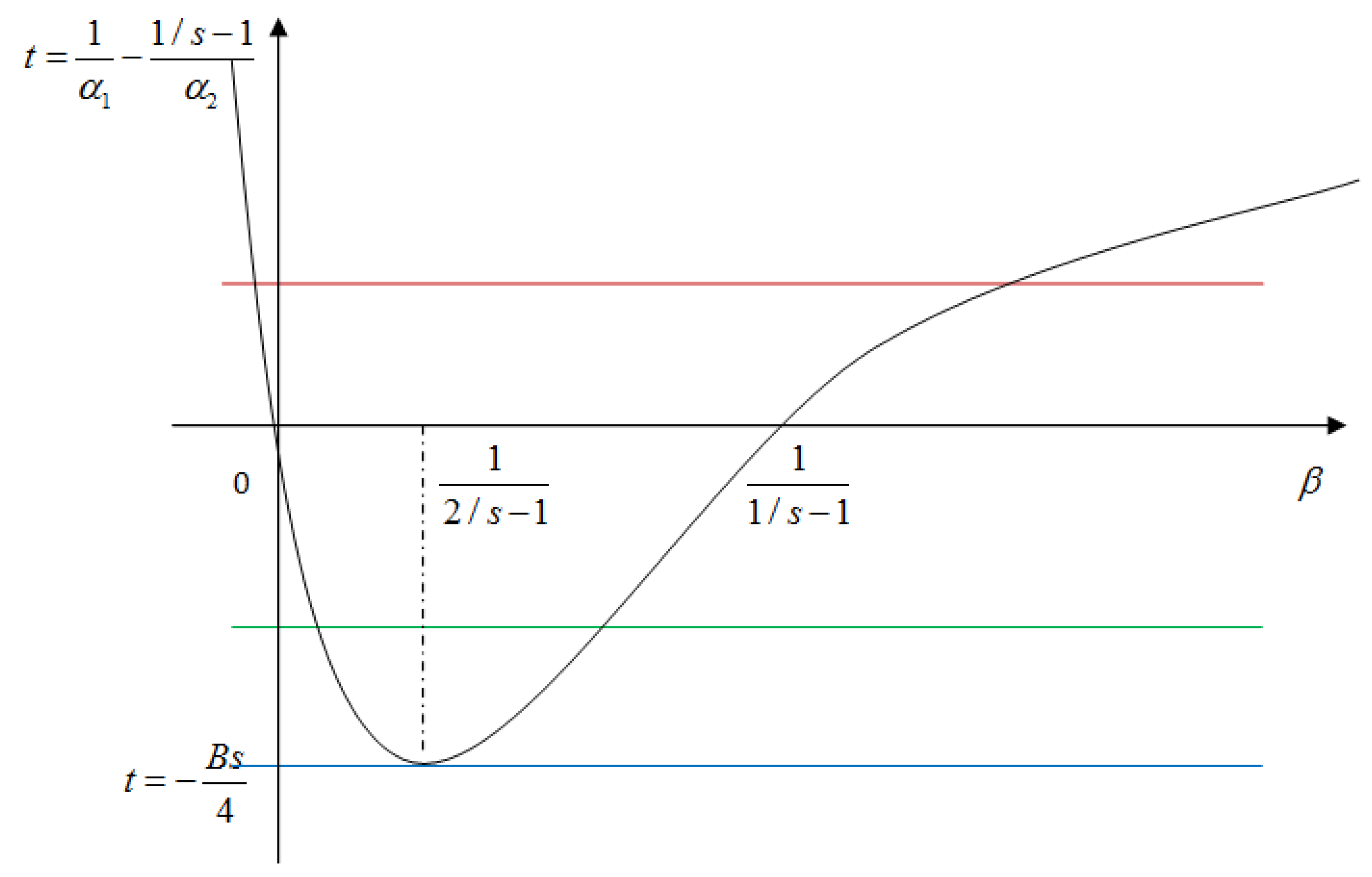
The shape of is convex first, then concave; and .
The graph of inequality is shown in Figure A1.
(1). If
Figure A1 shows that the whole curve is above the blue line; we have , which is sufficient condition for the referendum to satisfy supermajority requirement.
(2). If
Figure A1 shows that the curve above the green line is making inequality to hold, we have
which is sufficient condition for the referendum to satisfy supermajority requirement.
(3). If
Figure A1 shows that the curve above the horizontal axis is making inequality to hold, we have
which is sufficient condition for the referendum to satisfy supermajority requirement.
(4). If
Figure A1 shows that the curve above the red line is making inequality to hold, we have
which is sufficient condition for the optimal majority rule to satisfy supermajority requirement.
Figure A1.
Sufficient condition of Corollary 5.

References
- Rogoff, K. Opinion: The Brexit Vote Wasn’t Democratic at all. 2006. Available online: https://www.marketwatch.com/story/the-brexit-vote-wasnt-democratic-at-all-2016-06-27 (accessed on 30 May 2019).
- Qvortrup, M. A Comparative Study of Referendums: Government by the People, 2nd ed.; Manchester University Press: Manchester, UK, 2005; p. 171. ISBN 071907181X. [Google Scholar]
- Wicksell, K. A New Principle of Just Taxation, translated by Buchanan, James. In Classics in the Theory of Public Finance; Musgrave, R., Peacock, A., Eds.; Macmillan and Company: New York, NY, USA, 1994; pp. 72–118. [Google Scholar]
- Buchanan, J.; Tullock, G. The Calculus of Consent; University of Michigan Press: Ann Arbor, MI, USA, 1962. [Google Scholar]
- Rae, D.W. Decisions-rules and individual values in constitutional choice. Am. Political Sci. Rev. 1969, 63, 40–56. [Google Scholar] [CrossRef]
- Herrera, H.; Mattozzi, A. Quorum and Turnout in Referenda. J. Eur. Econ. Assoc. 2010, 8, 838–871. [Google Scholar] [CrossRef]
- Snyder, J.M. Election Goals and Allocation of Campaign Resources. Econometrica 1989, 89, 525–547. [Google Scholar] [CrossRef]
- Shachar, R.; Nalebuff, B. Follow the Leader: Theory and Evidence on Political Participation. Am. Econ. Rev. 1999, 57, 637–660. [Google Scholar] [CrossRef]
- Herrera, H.; Mattozzi, A. Quorum and Turnout in Referenda. SSRN Working Paper 2006. Available online: https://papers.ssrn.com/sol3/papers.cfm?abstract_id=1003803 (accessed on 30 May 2019).
- Osborne, J.M.; Turner, M.A. Cost Benefit Analyses versus Referenda. J. Political Econ. 2010, 118, 156–187. [Google Scholar] [CrossRef] [Green Version]
- Attanasi, G.M.; Corazzini, L.; Passarelli, F. Voting as a lottery. J. Public Econ. 2017, 146, 129–137. [Google Scholar] [CrossRef]
- Dal Bo, E. Committees with supermajority voting yield commitment with flexibility. J. Public Econ. 2006, 90, 573–599. [Google Scholar] [CrossRef]
- Messner, M.; Polborn, M. Voting on majority rules. Rev. Econ. Stud. 2004, 71, 115–132. [Google Scholar] [CrossRef]
- Kramer, G.H. The Effect of Precinct Level Canvassing on Voter Behavior. Public Opin. Q. 1971, 34, 560–572. [Google Scholar] [CrossRef]
- Wielhouwer, P.W.; Lockerbie, B. Party Contacting and Political Participation, 1952–1990. Am. J. Political Sci. 1994, 38, 211–229. [Google Scholar] [CrossRef]
- Spenkuch, J.; Toniatti, D. Political Advertising and Election Results. Q. J. Econ. 2018, 133, 1981–2036. [Google Scholar] [CrossRef]
- Bentley, A.F. The Process of Government: A Study of Social Pressures; Routledge: Abingdon-on-Thames, UK, 2017. [Google Scholar]
- Olson, M. The Logic of Collective Action; Harvard University Press: Cambridge, MA, USA, 2009. [Google Scholar]
- Coase, R.H. The Problem of Social Cost. J. Law Econ. 1960, 3, 1–44. [Google Scholar] [CrossRef]
- Munger, M. Kaldor-Hicks-Scitovsky Coercion, Coasian Bargaining, and the State. In Coercion and Social Welfare in Public Finance: Economic and Political Perspectives; Martinez-Vazquez, J., Winer, S., Eds.; Cambridge University Press: Cambridge, UK, 2014; pp. 117–140. [Google Scholar] [CrossRef]
- Why Vote Leave. Available online: http://www.voteleavetakecontrol.org/why_vote_leave.html (accessed on 30 May 2019).
| 1 | We thank an anonymous referee for encouraging us to add this broader discussion and suggesting the references to us. |
| 2 | Shachar and Nalebuff [8] point out, party spending is effective in driving voters to the polls in several ways: Campaign spending decreases the voters’ cost of acquiring information, it decreases the direct cost of voting, it increases the cost of abstaining, and it signals the closeness and importance of the alternatives at stake. |
| 3 | The mobilization functions should be viewed as the reduced form of more complex interactions between parties and the voters they represent. We abstract from the actual mechanism with which mobilization efforts translate into actual turnout, mindful of the caveat that turnout in a referendum itself requires justification that is beyond the scope of the paper. |
| 4 |
Figure 1.
Probability of approval.

Figure 2.
Pure-strategy Nash equilibrium for all value of majority rule .

Figure 3.
Relationship between and .


Table 1.
Majority provisions on referenda in established Western democracies *.
| Country | Majority Provisions on Referenda |
|---|---|
| Australia | Geographical requirement: Majority of votes and majority of states |
| Austria | Simple majority |
| Belgium | No provisions for referendums |
| Canada | Under debate |
| Denmark | Registered voter requirement: 30% of voters, 40% of voters on constitutional changes |
| France | Simple majority |
| Finland | Simple majority |
| Germany | No provisions for referendums |
| Iceland | Simple majority |
| Ireland | Simple majority |
| Italy | Turnout requirement: 50% of the registered voters |
| Luxembourg | Simple majority |
| Malta | Simple majority |
| Netherlands | Simple majority |
| Switzerland | Geographical requirement: Simple majority and majority of cantons |
| United Kingdom | Simple majority (40% of registered voters in 1979) |
| USA | No provisions for nationwide referendums |
* Source: Qvortrup [2], p.171.
Table 2.
Referenda with close results.
| Year | Referendum | Outcome | Turnout |
|---|---|---|---|
| 1972 | Norwegian European Communities membership referendum | 46.5–53.5% | 79% |
| 1992 | French Maastricht Treaty referendum | 49.0–51.0% | 69.7% |
| 1992 | The Danish Maastricht referendum | 49.3–50.7% | 83.1% |
| 1994 | Swedish European Union membership referendum | 52.3–47.7% | 83.3% |
| 1995 | The Quebec Secession referendum | 49.4–50.6% | 93.52% |
| 2001 | Nice I referendum | 46.1–53.9% | 34.8% |
| 2002 | Nice II referendum | 62.9–37.1% | 49.5% |
| 2005 | French European Constitution referendum | 45.3–54.7% | 69.4% |
| 2013 | San Marino-Sammarinese referendum | 50.3–49.7% | 43.38% |
| 2015 | The Danish European Union opt-out referendum | 46.9–53.1% | 72.0% |
| 2016 | The Brexit referendum | 51.9–48.1% | 72.2% |
© 2019 by the authors. Licensee MDPI, Basel, Switzerland. This article is an open access article distributed under the terms and conditions of the Creative Commons Attribution (CC BY) license (http://creativecommons.org/licenses/by/4.0/).
Share and Cite
MDPI and ACS Style
Cheng, Q.; Li, M. Optimal Majority Rule in Referenda. Games 2019, 10, 25. https://0-doi-org.brum.beds.ac.uk/10.3390/g10020025
AMA Style
Cheng Q, Li M. Optimal Majority Rule in Referenda. Games. 2019; 10(2):25. https://0-doi-org.brum.beds.ac.uk/10.3390/g10020025
Chicago/Turabian StyleCheng, Qingqing, and Ming Li. 2019. "Optimal Majority Rule in Referenda" Games 10, no. 2: 25. https://0-doi-org.brum.beds.ac.uk/10.3390/g10020025
Note that from the first issue of 2016, this journal uses article numbers instead of page numbers. See further details here.