Emotion and Knowledge in Decision Making under Uncertainty

Abstract

This paper presents four incentivised experiments analysing jointly the separate role of immediate integral emotions and knowledge in individual decision making under ambiguity. Reactions to a natural source of uncertainty (i.e., forthcoming real-world election results) were measured using both computed decision weights derived from individual choices and judgmental probabilities determined from the subjects’ estimated likelihood of election outcomes. This study used self-reports to measure emotions aroused by the prospective election victory of a party/coalition of parties, and both self-assessed and actual competence to measure knowledge of politics. This paper found evidence of both preference for ambiguity in the gain domain and of likelihood insensitivity, namely the tendency to overweight unlikely events and to underweight likely events. This paper also shows that a superior knowledge of politics was associated with a preference for ambiguity (i.e., the elevation of the decision weighting function for gains). Both stronger positive emotions and superior knowledge generally have asymmetric effects on likelihood insensitivity (i.e., the curvature of the decision weighting function), each being associated separately with higher overweighting of unlikely election outcomes.

1. Introduction

This paper presents four experiments that considered jointly the separate role of integral immediate emotions (i.e., emotions that are experienced at the time of decision and that are related to the decision at hand) and of knowledge (i.e., both self-assessed and actual knowledge of the decision context) in individual decision making under real-world ambiguity. The natural source of ambiguity was the set of possible shares of votes obtained by a party/coalition of parties in forthcoming political elections.

In the literature, the distinction between risk and uncertainty dates back to Knight (1921) [1] and Keynes (1921) [2]: Risk was associated with situations in which the likelihood of an event is known or “measurable” and uncertainty was associated with situations in which the likelihood of an event is not “measurable”. Ellsberg (1961) [3] (pp. 660–661) introduced a new definition that clarified the meaning of uncertainty: Probability may not be measurable either because the likelihood is unknown, or because there is conflicting, unreliable, vague, scanty or inexistent evidence and information on the possible occurrence of the considered event. To illustrate this effect, Ellsberg (1961) [3] used the two-colour two-urn paradox. A subject faces the simultaneous choice of a colour on which to bet and of an urn from which to draw a ball, whereby one urn contains 50 black and 50 red balls in known proportion (i.e., known probabilities), and the other urn contains 100 black and red balls in unknown proportion (i.e., unknown probabilities). Ellsberg called ambiguity aversion the preference to draw from the urn containing 50 black and 50 red balls, with the alternative showing ambiguity preference. Ellsberg’s definition does not necessarily imply that subjects use a second order probability distribution in order to represent themselves either the situation described in the urn with unknown composition or any other situation in which information is scanty or vague1. For this reason, following the literature on ambiguity (Camerer and Weber, 1992 [7]), this paper considered decision making on lottery events based on the results of political elections as an example of real-world ambiguity.

The aim of this paper was to disentangle the separate role that both emotion and knowledge can play in individual decision making under ambiguity, more specifically through their effects on the elevation and/or the curvature of the decision weighting function when ambiguity is generated by the outcome of real-world political elections. These are well-recognised, salient and powerful sources of emotional involvement (Brader and Marcus, 2013 [8]). In doing so, this paper adopted the theoretical framework of Cumulative Prospect Theory (Tversky and Kahnemann, 1992 [9] and Section 3). The paper shows that experimental student subjects exhibited a preference for ambiguity in the gain domain over lotteries based on political election outcomes and showed risk neutrality in choices under risk. Moreover, ambiguity preference was stronger when reaction to uncertainty was measured by using computed decision weights rather than judgmental probabilities. This paper also demonstrates that the difference between the sum of decision weights for complementary events and the corresponding sum of judgmental probabilities (which the paper interprets as a measure of uncertainty reaction that depends on a subject’s willingness to bet) was biased upwards by a superior knowledge of politics in two out of four experimental sessions. This result is consistent with Heath and Tversky’s (1991) [10] competence hypothesis, according to which superior knowledge of the decision context leads to more elevation of the decision weighting function for gains.

2. Review of the Literature

This section presents a review of the relevant literature, which is divided into three sub-sections: A brief review of the experimental evidence on the shape of the weighting function under ambiguity, a review on the role of emotion and, finally, a review on the role of knowledge in affecting such a shape.

2.1. The Shape of the Weighting Function under Ambiguity

In order to investigate the separate role that both emotions and knowledge can play in individual decision making under ambiguity, this paper used Cumulative Prospect Theory (CPT) as a reference model. In particular, this paper investigated the effects of these two variables on the shape of the probability weighting function, both in terms of elevation, as well as of curvature (i.e., so-called likelihood insensitivity or lower and upper subadditivity). Empirically, the shape of the probability weighting function under risk has been widely investigated (Tversky and Kahneman, 1992 [9], Wu and Gonzalez, 1996 [11], 1999 [12], Abdellaoui, 2000 [13]): The prevailing experimental finding is the inverse S-shaped weighting function, but there is wide heterogeneity at the individual level.

As far as ambiguity is concerned, Kilka and Weber (2001) [14] and Fox and Weber (2002) [15] compared reaction to ambiguity towards two sources of uncertainty, one more familiar than the other was. These authors found that subjects had a stronger reaction to ambiguity when the source was unfamiliar, and this reaction was revealed in different additivities of the probability weighting function. Using a two-stage approach in which they considered both probability judgements and decisions weights, Kilka and Weber (2001) [14] (pp. 1724–1725) concluded that “the properties of the probability weighting function were also significantly influenced by the source of uncertainty”and this influence affected the measure of additivity as well as the shape of the probability weighting function. More recently, de Lara Resende and Wu (2010) [16] provided further evidence of a knowledge effect on the elevation of the weighting function. Baillon and Bleichrodt’s (2015) [17] analysis confirmed the effect of source preference (risk vs. ambiguity), by finding a stronger violation of additivity under ambiguity relative to risk. However, their empirical results did not confirm that different sources of ambiguity (less vs. more familiar) were associated with a different elevation of the weighting function. As Abdellaoui et al. (2011) [18] pointed out, even if the prevailing empirical shape of the weighting function under ambiguity was the inverse S-shape, there was wide heterogeneity at the individual level with prevalence of ambiguity aversion, but also ambiguity seeking and insensitivity towards ambiguity, which is not surprising since ambiguity is a richer domain than risk.

2.2. Emotions

With regards to emotions, the literature on decision making makes a distinction between anticipated or expected emotions and anticipatory or immediate emotions (Loewenstein et al., 2001 [19] (pp. 267–268)). Anticipated emotions typically are emotions that people expect now to experience in the future when the outcomes will be observed, and that they perceive as expected consequences of their own decisions (such as regret and disappointment, Loomes and Sugden, 1982 [20], 1986 [21]). On the contrary, this paper considers integral immediate emotions (Rick and Loewenstein, 2008 [22] (pp. 138–139)). These are immediate visceral reactions that (i) are experienced at the time of decision and are unaffected by the choice that was made (immediate emotions), and (ii) are related to the decision at hand (integral emotions). More specifically, this paper considered people’s immediate feelings about the prospective victory of a party/coalition of parties in a forthcoming election while asking subjects to both price and assess the likelihood of different shares of votes for this party/coalition.

The role of immediate emotions in individual decision making has been overlooked in the economics literature, whereas it has played a prominent role in psychology. For example, the risk-as-feelings hypothesis (Loewenstein et al., 2001 [19]) interprets immediate emotions that may be aroused by outcomes as heuristics that motivate and determine choice directly. Building on evidence in psychology showing that the strength of immediate emotions is determined largely by both the vividness of the mental images of an outcome and by its temporal proximity to the moment of choice rather than by the likelihood of the outcome, the risk-as-feelings hypothesis posits that immediate emotions have an “all-or-none characteristic: they may be sensitive to the possibility rather than the probability” of the outcome. Therefore, one would expect that subjects dealing with affect-rich outcomes under risk would be very sensitive to probability variations at the endpoints of the probability scale but relatively insensitive at intermediate probability values. Rottenstreich and Hsee’s (2001 [23] (p. 187)) experimental evidence supports these predictions. In the gain domain, they found both more pronounced overweighting of low probabilities and more pronounced underweighting of high probabilities for risky lotteries associated with an affect-rich outcome (i.e., a coupon for a romantic trip) rather than with an affect-poor outcome (i.e., cash), other things being equal. Moreover, probability variations between 1% and 99% had a very limited impact on choice in the affect-rich case, but a big impact on choice in the affect-poor case. To explain their findings, Rottenstreich and Hsee (2001) [23] (p. 186, 189) argued that the affect-rich outcome elicited a more pronounced curvature of the decision weighting function (i.e., more likelihood insensitivity) than the affect-poor outcome, as long as it elicited hope of winning when the probability of winning was low and fear of losing when it was high. Alternatively, they argued that greater immediate emotions of savouring associated with the emotionally powerful positive outcome increased the elevation of the weighting function at each probability level, which, in their experiments, was exhibited as more overweighting of low probabilities. Ditto et al. (2006) [24] (p. 104) offered experimental evidence of the elevation effect at high probabilities for an affect-rich outcome (i.e., chocolate chip cookies) as well. More recently, Loewenstein et al. (2015) [25] (pp. 67–69) incorporated the risk-as-feelings hypothesis into a fully-fledged dual-process behavioural model of decision making. In their model, individual behaviour under risk results from the joint interaction of an affective system, which depends on the intensity of immediate emotions, and a deliberative system, which induces agents to behave as if they were Subjective Expected Utility Theory maximisers. Their model predicted that an increase in the degree of affect-richness of the outcome would lead to more likelihood insensitivity and especially, to an “excessive reaction to affectively charged but unlikely outcomes”.

It is worth noting that immediate emotions are neither necessarily associated with less than rational behaviour nor irrelevant for choice involving affect-poor money outcomes. Concerning the former issue, the valence of emotions matters (Damasio et al., 1994 [26]; Bechara, 2004 [27]; Slovic et al., 2004 [28]). On the one hand, positive emotions, by inducing subjects to rely on simpler heuristics, may signal that analytical processing is not needed. On the other hand, negative emotions, by signalling potential threats, may induce subjects to process available information more carefully (Schwarz, 2012 [29]), which facilitates rational thinking.

Regarding the role of immediate emotions when lotteries imply money outcomes, a few papers have recently shown that emotions influence the affect-richness of the decision context, hence individual choice. For example, Baillon et al. (2016) [30] found that subjects previously exposed to sad videoclips (i.e., a negative emotion) showed a more neutral attitude in choice under artificial uncertainty than subjects previously exposed to joyful (i.e., a positive emotion) videoclips. Schlösser et al. (2011) [31] (p. 37) showed that the preference for betting on an Ellsberg’s urn with unknown rather than known probabilities (hence, the preference for ambiguity vs. risk) was stronger for subjects who “felt more positive, aroused and in control about gambling”. Li et al. (2018) [32] (pp. 3234, 3237) showed that if the decision context was expected to arouse immediate positive emotions (as in their “kid charity treatment”), experimental subjects displayed lower ambiguity aversion and lower likelihood insensitivity (i.e., lower overweighting of low likelihoods and lower underweighting of high likelihoods) than when they evaluated affect-poor Ellsberg’s urn lotteries. These authors explained their results in terms of an emotion-generated elevation effect of the decision weighting function, akin to Heath and Tversky’s (1991) [10] competence-generated elevation effect (see below). They argued that positive emotions aroused by the kid-charity decision context generated extra general utility, which showed up as a more elevated decision weighting function in their data.

Similarly to the above-mentioned papers, the first aim of the current paper was to analyse the role of integral immediate emotions in individual choice under uncertainty when the decision context (i.e., forthcoming elections) is expected to arouse both positive and negative emotions, and uncertain lotteries are associated with a fixed money outcome (see Section 4 and Supplementary Materials). The idea is that although emotions elicited by the electoral decision context did not affect either the monetary outcome or likelihoods, they could affect choice and thus, the shape of the decision weighting function.

2.3. Knowledge

The second aim of the current paper was to analyse the role of knowledge in decision making under ambiguity. In particular, by using both self-reports and objective measures of the political context associated with each election (see Section 4 and Supplementary Materials), this paper attempted to investigate the role of knowledge over the value function, and in particular, over the weighting function used to evaluate lotteries under real-world ambiguity. The idea that competence may have an effect on the perception of uncertainty was first introduced by Heath and Tversky (1991) [10]. According to the competence hypothesis, when experts on a topic (e.g., football, politics), subjects may prefer to bet on an event lottery (i.e., on an ambiguous lottery) than on a risky lottery with equivalent probability, showing, in this case, ambiguity preference. In terms of decision weights, this preference can be translated into a higher elevation of the weighting function and in the fact that the sum of the decision weights for complementary events is higher under ambiguity than under risk. Fox and Tversky (1995) [33] and Tversky and Fox (1995) [34] extended this investigation to the comparison between two different sources of ambiguity, one more familiar and the other less familiar. The experimental evidence showed that in the domain of gain, subjects preferred to bet on more familiar sources of ambiguity—for which they had or felt to have more competence, and/or more knowledge or understanding of the relevant decision context—than on less familiar sources. Examples include the preference to bet on variations in stock exchange indexes, on the results of sporting or electoral contests, and on city temperatures that were more familiar relatively to less familiar or unfamiliar sources (Keppe and Weber, 1995 [35], Fox and Tversky, 1998 [36], Di Mauro and Maffioletti, 2001 [37]; but see Baillon and Bleichrodt, 2015 [17], for mixed evidence). Competence-driven source preference may be translated into a more elevated S-shaped decision weighting function at each likelihood level for the more familiar than the less familiar source (de Lara Resende and Wu, 2010, [16] (p. 128), Abdellaoui et al., 2011 [18] (p. 313)). However, since the experimental evidence showed mixed results and heterogeneity of behaviour (Abdellaoui et al., 2011 [18]), one needs more investigation on the topic. In particular, as Fox and Weber (2002) [15] (p. 495) pointed out, source preference and likelihood insensitivity (which they termed source sensitivity) are “logically independent”. Hence, it is not surprising that the experimental evidence found no clear association between these two features of behavioural reaction to uncertainty.

What is the rationale for the elevation effect associated with source preference? Heath and Tversky’s (1991 [10] (pp. 7–8) competence hypothesis posited that people considering themselves experts or being actual experts prefer betting on the familiar source as long as, beside the monetary payoffs, they derived “physic payoffs of satisfaction from correct predictions, while minimising or avoiding embarrassment from wrong predictions”. Chew et al.’s (2008 [38] (pp. 195–196) neuroimaging experiment validated the hypothesis that choosing a more familiar source of ambiguity was more rewarding, thus generating extra utility. Fox and Tversky (1995 [33]) further argued that the feeling of competence or knowledge arises from the comparative assessment subjects make between different sources (or between individuals with different knowledge). Therefore, according to this comparative ignorance hypothesis, the preference for betting on the familiar source of events should taper off when subjects evaluate different sources in isolation rather than jointly, given that, in the former case, one’s degree of competence becomes less salient for choice. However, Fox and Weber (2002) [15] (p. 479, pp. 487–488) pointed out that what matters is “the state of mind of the decision-maker rather than the experimental manipulation context”. This means that comparative assessment can operate even when the experimental context is not explicitly comparative, which is the case of the current paper.

3. Theoretical Background

This Section presents the theoretical background that may be useful to interpret this paper’s results. However, the non-interested reader can jump directly to the testable hypotheses at the end of this Section.

According to the Cumulative Prospect Theory (CPT, Tversky and Kahnemann, 1992 [9]), the value function of a risky binary lottery paying €x with probability p and paying nothing otherwise is V(z) = w(p)v(x), where z is the minimum selling price and w denotes the decision weight. Provided the value function for monetary gains is linear (see Section 5.1 below), one can use the ratio between each subject’s minimum selling price and the money outcome of the lottery to compute the weighting function for risk at each probability level: w(p) = z/v.

Under ambiguity, the value of a simple binary prospect yielding outcome x if uncertain event A occurs (here, a positive amount of money given a determined share of votes) and outcome 0 otherwise, can be represented by V(A, x) = W(A)v(x), where W denotes the decision weight (also termed capacity) associated with the occurrence of A, and v(.)—with v(0) = 0 and v’ > 0—is the value function of money x. Assuming linearity v(x) = x, the ratio between the minimum selling price and the money outcome of the lottery yields the subject’s decision weight associated with uncertain event A.

Moreover, under ambiguity, the sum of decision weights for complementary events and similarly the sum of judgemental probabilities provides a measure of reaction to ambiguity under CPT (see Section 5.3 below). Following Baillon and Bleichrodt (2015) [17], one has tertiary additivity (TA)2 when the state space is partitioned in three or more than three mutually exclusive and disjoint complementary events; whereas one has binary complementary (BC) when the state space is partitioned in two mutually exclusive and disjoint complementary events. If subjects follow the Subjective Expected Utility Theory (SEUT) or probabilistic sophistication (Machina and Schmeidler, 1992 [39]), the sum of computed decision weights—or the sum of judgemental probabilities—for complementary events, thus the corresponding additivity test, takes a value of unity. Values of the additivity test different from unity can be taken as evidence of reaction to ambiguity. More specifically, as long as subjects’ probabilities sum up to one under risk (see Section 5.2 below), one can argue that if the sum of decision weights/judgmental probabilities under ambiguity is greater than unity, a subject exhibits ambiguity preference. If the sum is less than unity, s/he exhibits ambiguity aversion instead.

Under CPT, the weighting function is also characterised by Lower and Upper Subadditivity from which one can derive the before mentioned property of likelihood insensitivity, a well-documented dimension of reaction to ambiguity (see Section 2.1). This property implies that in the gain domain, subjects simultaneously exhibit a tendency to overweight low likelihoods and to underweight high likelihoods, while being less sensitive to intermediate likelihood variations. Following Tversky and Fox (1995) [34] (p. 272), these features can be captured using the concept of bounded subadditivity (BA). BA satisfies the following properties for decision weights under ambiguity:

(i)

Lower Subadditivity (LSA):

$$\mathrm{WLSA} = \mathrm{W}\left(\mathrm{A}\right)+\mathrm{W}\left(\mathrm{B}\right)-\mathrm{W}(\mathrm{A}\cup \mathrm{B})\ge 0, \mathrm{provided} \mathrm{A}\cap \mathrm{B} = \varnothing \mathrm{and} \mathrm{W}(\mathrm{A}\cup \mathrm{B}) < 1.$$

(ii)

Upper Subadditivity (USA):

$$\mathrm{WUSA} = 1-\mathrm{W}(\mathrm{S}-\mathrm{A})-\mathrm{W}(\mathrm{A}\cup \mathrm{B})+\mathrm{W}(\mathrm{B})\ge 0, \mathrm{provided} \mathrm{A}\cap \mathrm{B} = \varnothing \mathrm{and} \mathrm{W}\left(\mathrm{B}\right) > 0$$

WLSA denotes the possibility effect, i.e., the fact that adding an event A to the null event has more impact than subtracting it from some non-null event. WUSA captures the certainty effect, i.e., the fact that subtracting an event A from the certain event S has more impact than subtracting it from some uncertain event $\mathrm{A}\cup \mathrm{B}$. If subjects behave according to SEUT, WLSA = WUSA = 0. If they are likelihood insensitive, they will overweight unlikely events, which implies that WLSA > 0 and they will underweight likely events, which implies that WUSA > 0. If these properties hold, the weighting function will be inverse S-shaped. For judgemental probabilities, BA is defined similarly (Tversky and Fox, 1995 [34] (p. 279)). These properties proved to be relevant to interpret the results of Section 5.4 below.

Borrowing from Tversky and Fox (1995) [34] and Fox and Tversky (1998) [36], we posited that subject i = 1 … N evaluates ambiguity in a two-stage process in which s/he first assesses the probability J of an uncertain event A, then transforms J into the decision weight W. Fox and Tversky (1998) assumed that W equals to W(Ai) = wR(J(Ai)), where w_R stands for risk. Following Kilka and Weber (2001), we extend the interpretation of w to ambiguity, so that w can encompass decision weights under risk as well as under ambiguity. Moreover, the judgmental probabilities J have similar properties to those of the weighting functions, namely BC, TA and BA.

In order to investigate not only reaction to ambiguity when ambiguity is represented by a real-world event, but also to allow for the influence of emotion and knowledge on decision making under ambiguity, we modified the weighting function. In particular, we adopted the following specification W(A, e_i, k_i) = W(J(A, k_i), e_i, k_i), where e_i denotes the strength of immediate emotions elicited by elections, and k_i is individual i’s degree of subjective or objective knowledge or understanding of the electoral context. Hence, the decision weight W can be decomposed into a belief component, i.e., the subjective degree of belief J, which can be affected directly by knowledge (as documented by Kilka and Weber, 2001 [14]) and a decision attitude or willingness to bet component, which is potentially affected by immediate emotions and knowledge. The belief component was measured experimentally by asking subjects to state their judged probabilities J for the uncertain event A. The decision weight W was inferred from a subject’s stated certainty equivalent for the same event and computed as the ratio between the minimum selling price and the prize of that lottery.

Based on the theoretical background, the following testable hypotheses are formulated:

Hypotesis 1 (H1).

Source preference. We expect subjects to evaluate lotteries under risk differently from lotteries under ambiguity. We expect that this difference (whichever direction it takes: ambiguity preference or aversion) will be stronger for the decision weights than for the judgemental probabilities.

We empirically measured Hypothesis 1 through binary complementarity and tertiary additivity as well as through lower and upper subadditivity. Hence, if a subject is ambiguity averse, say, the sum of her decision weights for complementary events will be less than the sum of her judgemental probabilities. This is also revealed through differences in lower and upper subadditivity when considering the decision weights and the judgemental probabilities.

Hypotesis 2 (H1).

Influence of emotion and knowledge on ambiguity reaction. We expect stronger emotion and a superior knowledge of the decision context to enhance the difference between the decision weights and the judgmental probabilities. Besides, we expect each variable to affect likelihood insensitivity, namely to change the elevation and the shape of the weighting functions and of the judgemental probabilities.

Hypothesis 2 was empirically measured in a two-fold way. First, we looked for a possible correlation between the difference between decision weights and judgemental probabilities, W-J, and the level of emotion and knowledge. For example, following Heath and Tversky 1991 [10], one would expect that a superior knowledge will increase this difference either through an increase of preference for ambiguity (i.e., increasing the willingness to bet over the ambiguous lotteries) or by reducing the distortion over the probability judgement. Besides, following the empirical result of Rottenstreich and Hsee (2001) [23], one would expect stronger emotions also to influence the difference W-J, for example by increasing ambiguity preference for positive emotions.

Second, we measured the effect of knowledge and emotion through the influence of the two variables over the elevation of the weighting function, that is through their potential effect in increasing or decreasing the lower and upper subadditivity, namely the overweighting and the underweighting of probabilities. In particular, following previous experimental results, one would expect, as in Kilka and Weber (2000) [14], that subjects became more optimistic when they felt more competent, and, as in Rottenstreich and Hsee (2001), when positive emotions were involved.

4. Experimental Design and Methods

This section presents the details of the experimental design, which followed Fox et al. (1996) [40] and Kilka and Weber (2001) [14]. We run four experiments using the same within-subject design. All the subjects had to perform four tasks: a matching task (i.e., stating the amount of money that made them indifferent between two lotteries), two pricing tasks (one for risk and the other for ambiguity), and a self-evaluation of probabilities for ambiguous lotteries (considering the same lotteries used for the pricing task). Moreover, the subjects had to assess their emotional involvement in case of ambiguity and either self-assess their knowledge in politics or answer some politics-related questions. At the end of the experiment, they filled in an anagraphical questionnaire. The experiments were conducted with pencil-and-paper. They lasted about one hour, and subjects met in a room (see Supplementary Materials).

Table A1. Experiments.

Experiment	Election	Recruitment	Subjects	Date Exper.	Incentives
Milan 1	13 May 2001 Italian general political election.	Volunteers recruited through advertisement at the Faculty of Political Science of the University of Milan.	Subjects = n. 35 Females = n. 12 Males = n. 23 Median age = 25.37 s.d. age = 3.79	10 May 2001	Show-up fee: 2000 Italian liras (about €1) instant lottery ticket. Incentive: Up to 240,000 Italian liras (about €120) if randomly selected.
Alessandria	12 and 13 June 2004 European parliamentary election.	Volunteers recruited through advertisement at the Faculty of Political Science of the University of Eastern Piedmont (IT).	Subjects = n. 31 Females = n. 14 Males = n. 17 Median age = 23.77 s.d. age = 3.68	9 June 2004	Show up fee: €3 instant lottery ticket. Incentive: Up to €120 if randomly selected.
Milan 2	23 and 24 February 2013 Italian general political election.	Volunteers attending an UG Public Economics course at the Faculty of Political, Economic and Social Sciences (SPES) of the University of Milan.	Subjects = n. 32 Females = n. 17 Males = n. 15 Median age = 24.84 s.d. age = 8.84	20 February 2013
Milan 3	4 March 2018 Italian general political election	Volunteers attending an UG Public Economics course and a Graduate Macroeconomics course at the Faculty SPES of the University of Milan.	Subjects = n. 21 Females = n. 6 Males = n. 15 Non-Italian = n. 7 Median age = 23 s.d. age = 1.43	1 March 2018 (UG) 2nd March 2018 (Graduate)

in Appendix A summarises the number and main characteristics of the subjects, the recruitment procedures and the incentives used in each experiment. We run each experiment a few days before the election contests: Milan 1 corresponded to the 2001 Italian general political election, Alessandria to the 2004 European parliamentary election, Milan 2 to the 2013 Italian general political election, and Milan 3 to the 2018 Italian general political election. All the subjects were volunteer Italian students, except for seven volunteer non-Italian students in Milan 3. Graduate students participated in Milan 3 only. Overall, 119 subjects participated to the four experimental sessions.

The first two sets of questions (i.e., the matching task and the pricing task under risk) were exactly the same in all the experiments.

Matching task: Each subject compared two pair of lotteries with different prizes and probabilities and wrote the amount of money making her/him indifferent between each pair. If the subject wrote the amount of money making the two lotteries equal in expected value, this was taken as evidence of a linear value function for this task (see Appendix A and Supplementary Materials).

Pricing task under risk: In the pricing task, each subject evaluated nine risky prospects at probability levels from 0.1 to 0.9 in increments of 0.1. These were presented as a random draw of a single ball from an opaque bag containing ten two-colour balls, with one positive outcome of 120,000 Italian liras in Milan 1, and of €60 in Alessandria, Milan 2 and 3 (see Appendix A and Supplementary Materials). The risky prospects were used for deriving decision weights under risk.

Pricing task under ambiguity: This constituted the third set of questions in each experiment and was experiment specific, as far as the subjects had to price ambiguous prospects based on political election outcomes (i.e., four experiments for four elections). The subjects reported their minimum selling price for nine lotteries. We based the lotteries on the share of votes a centre-right party/coalition of parties was expected to poll in a forthcoming election. Each uncertain lottery paid 120,000 Italian liras in Milan 1, €60 in Alessandria, Milan 2 and Milan 3, if the centre-right party/coalition of parties had obtained a given share of votes and nothing otherwise.

Table 1. Uncertain lotteries for Milan 3.

Pricing Question	Judgment of Probability Question
On Sunday the 4 March 2018, the Italian general elections will be held. You own a ticket of the following lottery: You win €60 if the Centre-Right coalition (Forza Italia-Berlusconi, Lega-Salvini premier, Fratelli d’Italia-Meloni, Noi con l’Italia-UDC) wins X% of the votes at the national level for the Chamber of Deputies, otherwise you win nothing. What is the minimum selling price at which you are willing to sell your lottery ticket? Price=	On Sunday the 4 March 2018, the Italian general elections will be held. The Centre-Right coalition (Forza Italia-Berlusconi, Lega-Salvini premier, Fratelli d’Italia-Meloni, Noi con l’Italia-UDC) wins X% of the votes at the national level for the Chamber of Deputies. Probability estimate=
The target events X% were as follows: A = less than 35% [or between 0% (included) and 35% (excluded)]; B = between 35% (included) and 38% (excluded); C = between 38% (included) and 40% (excluded); D = at least 40% [or between 40% and 100% (both included)]; E = between 35% (included) and 40% (excluded); F = less than 40% [or between 0% (included) and 40% (excluded)]; G = at least 35% [or between 35% and 100% (both included)]; H = at least 38% [or between 38% and 100% (both included)]; I = less than 38% [or between 0% and 38% (excluded)]

reports questions and shares of votes/target events for Milan 3. See the Appendix A for the other elections.

For each election, we selected nine shares of votes/target events based on the latest opinion polls published in the Italian national press. As a result, we created seven different space partitions for complementary lotteries covering the full space of events (100% of votes) for each election: A + B + C + D; A + B + H, A + E + D, C + D + I, F + D; A + G; H + I. (See Table 1 for Milan and Appendix A for Milan 1, Alessandria and Milan 2 event partition). We designed these questions to derive decision weights from individual preferences under ambiguity.

Evaluating judgemental probabilities: In each experiment, subjects also stated their probability judgments for the same prospects used in the pricing task under ambiguity. In Milan 3, for example, they had to state their judgmental probabilities for all the states of the world reported in the bottom half of Table 1 and for all partitions of the events space. Note that the state partition was the same for all the experiments, but it corresponded to different events, which were experiment specific. (See the Appendix A for the other experiments). These latter questions were aimed at eliciting the subjects’ degree of belief/subjective probability independently of the choice determinants related to the decision context and that show up in the computed decision weights (Wakker, 2004 [41]).

Scale rating: In all the experiments, we used a scale rate to measure emotional involvement. We used a single self-rating 11-point scale ranging from zero (no emotional involvement or neutral feeling) to ten (highest emotional involvement) for both positive emotions and negative emotions. Moreover, we measured in the same way the level of satisfaction related to a prospective “victory” of a centre-right party/coalition of parties. We designed these questions to capture immediate emotions associated with the decision context.

We also used a scale rating of the same type to measure self-assessed knowledge of the decision context. In particular, we used a single self-rating 11-point Likert scale ranging from zero (no expertise) to ten (very expert) in Milan 1, Milan 2, and Milan 3.

Table A2. Self-report questions in Milan 3.

Emotion

Knowledge

Consider the case in which the Centre-Right coalition (Forza Italia-Berlusconi, Lega-Salvini premier, Fratelli d’Italia-Meloni, Noi con l’Italia-UDC) polls the relative majority of votes in the Italian general political elections. On a scale between 1 and 10 state your level of positive emotional involvement* for this result, 0 showing the lowest positive emotional involvement *, 10 the highest positive emotional involvement *: 0---1---2---3---4---5---6---7---8---9—10

Do you rate yourself an expert in politics? On a scale between 1 and 10, report on the level of knowledge and expertise that you feel having as regards politics (0 not at all an expert, 10 very expert). 0---1---2---3---4---5---6---7---8---9--10

Note: * negative emotional involvement/level of of satisfaction.

in Appendix A shows the typical questions for Milan 3. In addition to self-assessed knowledge, in Alessandria, Milan 2 and Milan 3 knowledge was also measured by using a 10-question politics questionnaire: In this case the degree of objective knowledge for each agent was derived as the number of correct answers (see Appendix A for the questionnaires).

Order of presentation of tasks. In each experiment, the subjects undertook the matching task first. To avoid order effects, the sequence of the remaining tasks (pricing risky prospects, pricing and probability judgments for ambiguous prospects, emotional involvement and knowledge questions) was presented in a random order to subjects. Moreover, the order of presentation was randomised for each subject within tasks. Questionnaires were in Italian for Milan 1, Alessandria and Milan 2, whereas Milan 3′s questionnaire was in English (see Section 5.4 below for a discussion).

Incentive mechanism. At the end of each experiment, about one out of ten participants were randomly selected for real money play. A few days after each election, the selected subjects met in a room and two questions among the matching, risky and pricing questions were randomly drawn from an opaque bag. The experimenter’s offer for each lottery was generated randomly following the Becker, DeGroot and Marschak (1963) [42] procedure: If the offer was equal to or greater than the subject’s stated selling price for that lottery, the experimenter paid her offer to the subjects. Otherwise, the lottery was played for real according to the subjects’ answers. This mechanism, selecting multiple lotteries randomly, was incentive-compatible as long as subjects had no incentive to report their selling prices untruthfully. Accordingly, four subjects were selected in Milan 1, receiving an average payoff of 110,000 Italian liras (about €55); four subjects were selected in Alessandria, receiving an average payment of €104; three selected subjects received €53 on average in Milan 2, whereas each of the two selected subjects received €120 in Milan 3. We are confident that our subjects understood the incentive mechanism that was well explained with examples when reading the written instructions (see Supplementary Materials) before subjects evaluated the various scenarios. Note that, as long as the subjects’ prospective gains were independent from their self-reported levels of emotions and knowledge and from their judgemental probabilities (namely, they knew that only the matching, risky and uncertain lotteries were going to be played for real), we believe that they had no incentive to misrepresent their preferences. Hence, these questions were not incentivised.

5. Results

5.1. Matching Tasks

As we described in Section 4, the two matching tasks were designed to measure the utility of money under risk. At median values, matching tasks provided evidence of a linear value function for monetary gains. In all the experiments, but Milan 3, linearity was satisfied in both matching tasks (i.e., the median value across subjects was equal to the amount of money making the two lotteries indifferent in expected value)3. Based on this evidence, the paper shall assume a linear value function at the individual level in each experimental session. This assumption is consistent with studies showing that the utility function is approximately linear for small and moderate gains (Wakker and Deneffe, 1996 [43]; Abdellaoui et al., 2005 [44] (pp. 1390–1391), Booij et al., 2010 [45] (p. 134)), which is our case.

5.2. Decision Making under Risk

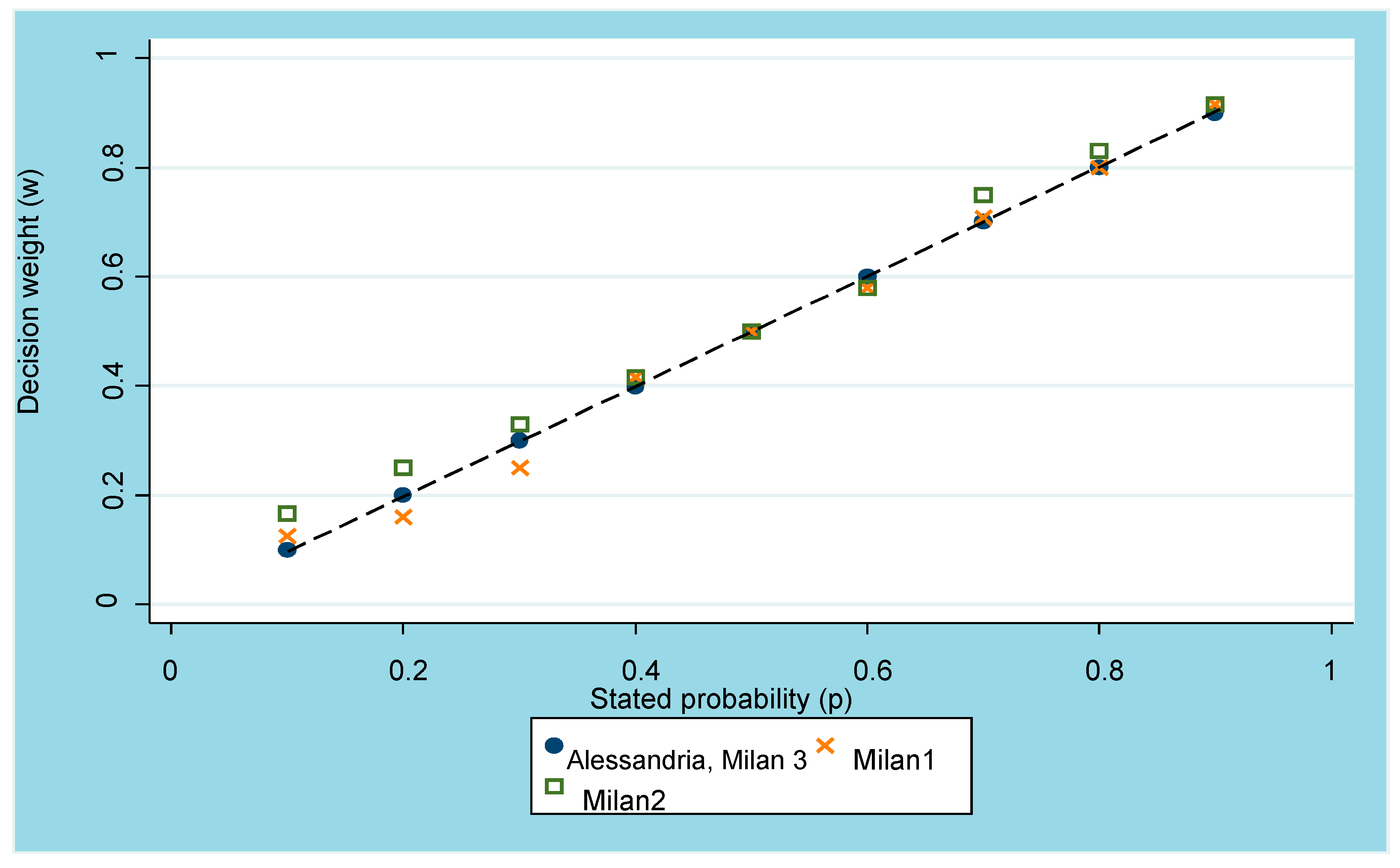
To assess subjective probability functions under risk, in each experimental session each subject had to state her/his minimum selling price for nine risky prospects, consisting in drawing a white ball from an opaque bag containing ten black and white balls in known proportions from 0.1 to 0.9 in increments of 0.1. Each lottery payed a fixed amount of money x if the white ball was drawn and payed nothing otherwise. (See Appendix A and Supplementary Materials.) Assuming linearity of the utility function (see above), we can calculate the weighting function as w (p) = z/x. Figure 1 below plots the median values at each probability level.

Median decision weights were equal to the objective probabilities in Alessandria and Milan 3 (see the dots) and very close to the objective probabilities in both Milan 1 (see the crosses) and Milan 2 (see the squares): at median values, subjective probabilities summed up to one.

These results provide evidence of a linear weighting function and allow us to conclude that in our experiments subjects are probability sophisticated under risk, showing equal sensitivity to changes in objective probabilities. Fox et al. (1996) [39] found a similar result for option traders. As a consequence, the existence of lower and upper subadditivity and the non-additivity in probabilities is sufficient to prove source preference as stated in Hypothesis 1 above.

5.3. Decision Making under Ambiguity

As we already discussed, in each experiment, corresponding to different Italian elections, each subject reported her/his minimum selling price for nine binary lotteries, each lottery paying a given amount of money if a centre-right party/coalition of parties gained a stated share of votes in a forthcoming election. This generated seven different space partitions for complementary lotteries covering the full space of events (100% votes; see Table 1 and Appendix A). We also asked subjects to report the corresponding judgement of probability for the same lotteries.

Assuming linearity, as in the case of risk, decision weights under ambiguity can be computed as w(p) = z/x. In other words, the ratio between the minimum selling price and the money outcome of the lottery provides the subject’s decision weight associated with the uncertain event. As stated in Section 5.2, given that our subjects exhibited probability sophistication under risk, the mere existence of non additivity in probabilities (i.e., sum of probabilities different from 1) can be seen as evidence of source preference according to Hypothesis 1.

We computed tertiary additivity (TA) (corresponding here to partitions: A + B + C + D, A + B + H, A + E + D, C + D + I) and binary complementary (BC, corresponding here to partitions: A + G, F + D, H + I) to investigate whether subjects showed ambiguity preference or ambiguity aversion, as defined and explained in Section 3. In fact, the sum of decision weights for complementary events, and similarly, the sum of judgemental probabilities provides a measure of reaction to ambiguity under CPT.

Table 2. Uncertain lotteries: Median values across individuals of the additivity tests.

Additivity Tests	Space Partitions	Median Sum of Decision Weights				Median Sum of Judgmental Probabilities
		(a)	(b)	(c)	(d)	(e)	(f)	(g)	(h)
		Milan 1 N = 35	Alessandria N = 31	Milan 2 N = 32	Milan 3 N = 21	Milan 1 N = 35	Alessandria N = 31	Milan 2 N = 32	Milan 3 N = 21
Tertiary additivity	A + B + C + D	1.83	2	1.63	1.7	1.7	1.75	1.5	1.7
	A + B + H	1.42	1.67	1.33	1.39	1.2	1.4	1.3	1.45
	A + E + D	1.5	1.67	1.33	1.42	1.2	1.38	1.3	1.4
	C + D + I	1.54	1.58	1.33	1.5	1.7	1.35	1.33	1.29
Binary Complementarity	A + G	1.08	1.17	1.03	1.08	0.9	1	1	1.15
	F + D	1.08	1.17	1	1	1.15	1	1	1.1
	H + I	1.17	1.33	1	1.08	1.15	1	1	1.1

Note: Each cell reports the median sum of decision weights and judgmental probabilities for each space partition across subjects. As long as subjects showed risk neutrality (see Figure 1), a median sum equal to unity, greater than unity or less than unity was taken as evidence of neutrality to, preference for, and aversion to ambiguity, respectively. See Table 2 and Appendix A for definitions of the space partitions in each experiment.

below reports the median value across subjects of the sum of decision weights and judgmental probabilities for each additivity test. In all the experiments, the median sum of decision weights exceeded unity for TA. These results support Hypothesis 1 of source preference. Table 2 also shows that the median sums generally increased in the number of space partitions. As far as BC is concerned, we can observe that it is very close to one for decision weights, while it is almost equal to one for judgemental probabilities4.

Table A3. Percentage of subjects violating additivity.

Tests	Space Partitions	Percentage of Subjects with Sum of Decision Weights Greater (Less) than Unity				Percentage of Subjects with Sum of Judgemental Probabilities Greater (Less) than Unity
		(a)	(b)	(c)	(d)	(d)	(e)	(f)	(g)
		Milan 1 N = 35	Ales_Sandria N = 31	Milan 2 N = 32	Milan 3 N = 21	Milan 1 N = 35	Ales_Sandria N = 31	Milan 2 N = 32	Milan 3 N = 21
Tertiary additivity	A + B + C + D	94 (3)	96.7 (3.3)	87.5 (12.5)	95 (5)	88.5 (3)	93.5 (6.4)	87.5 (3.1)	100 (0)
	A + B + H	88.5 (5.7)	87 (3.3)	65.6 (18.8)	80.9 (9.5)	63 (34.3)	87 (6.4)	68.7 (15.6)	95 (0)
	A + E + D	88.5 (8.5)	87 (3.3)	71.8 (18.8)	85.7 (9.5)	74.3 (8.5)	83.8 (12.9)	62.5 (28.1)	90.4 (5)
	C + D + I	85.7 (8.5)	87 (3.3)	78.1 (18.8)	90.4 (5)	88.6 (3)	80.6 (6.4)	71.8 (15.6)	95 (5)
Binary complementarity	A + G	45.7 (28.5)	64.5 (16.1)	37.5 (43.7)	43 (28)	26 (51.4)	35.4 (19.3)	25 (31.2)	57 (9.5)
	F + D	45.7 (22.8)	70.9 (12.9)	37.5 (46.8)	38 (38)	60 (20)	29 (22.5)	40.6 (18.7)	57 (14)
	H + I	54.3 (28.5)	70.9 (12.9)	34.3 (37.5)	57 (19)	57 (25.7)	42 (35.4)	34.3 (31)	47.6 (28.5)

Note: The residual in each cell (not shown) represents the proportion of subjects satisfying the additivity tests. See Table 2 in the main text and this Appendix A for definitions of the space partitions in each experiment.

in Appendix A reports the proportion of subjects violating each additivity test: these data also support the hypothesis of source preference. In fact, a large proportion of subjects exhibited preference for ambiguity (i.e., a sum greater than unity).

As previously argued, likelihood insensitivity is an important feature of the weighting function and a well-documented dimension of reaction to ambiguity (see Section 2 and Section 3): It implies a tendency to overweight low likelihoods and underweight high likelihoods, while being less sensitive to intermediate likelihood variations. In addition, we can use this dimension to test the hypothesis of source preference. In particular, as long as likelihood insensitivity can be captured using the concept of bounded subadditivity (BA, Tversky and Fox, 1995 [34] (p. 272) and Section 3 above), a different BA between decision weights under risk and under ambiguity can be interpreted as evidence of ambiguity reaction. Given that our subjects exhibited probability sophistication under risk, the mere existence of BA for the ambiguous lotteries can be taken as evidence of reaction to ambiguity in our experiments. For this reason, we computed lower subadditivity (LSA) and upper subadditivity (USA) tests, using the space partitioning of the lotteries corresponding to the experimental scenarios5.

Table 3. Lower subadditivity (LSA) and upper subadditivity (USA): Median values across subjects.

	Milan 1	Alessandria	Milan 2	Milan 3
Decision weights	wlsa = 0.42 wusa = 0.25 sw = 0.33	wlsa = 0.33 wusa = 0.17 sw = 0.42	wlsa = 0.17 wusa = 0.28 sw = 0.33	wlsa = 0.33 wusa = 0.25 sw = 0.42
Judgmental probabilities	jlsa = 0.3 jusa = 0.2 sj = 0.45	jlsa = 0.3 jusa = 0.25 sj = 0.35	jlsa = 0.24 jusa = 0.2 sj = 0.5	jlsa = 0.3 jusa = 0.2 sj = 0.57

Note: This table shows the median value of the individual medians for the index of lower subadditivity, upper subadditivity and global sensitivity for decision weights and judgmental probabilities. wlsa and jlsa: median value of each individual median lower subadditivity index; wusa and jusa: median value of each individual median upper subbaditivity index; sw = 1-wlsa-wusa, and sj = 1-jlsa-jusa, global sensitivity indexes. Bounded subadditivity is satisfied when wlsa > 0, wusa > 0, sw < 1; jlsa > 0, jusa > 0, sj < 1.

shows the median values of the individual medians across the various tests—denoted wlsa, wusa, jlsa, jusa. BA is satisfied, for example, when wlsa ≥ 0, wusa ≥ 0, whereas expected utility holds when wlsa = wusa = 0. Table 3 also reports a measure of global sensitivity, sw = 1-wlsa-wusa, computed by using the first three indexes of LSA and USA: the smaller sw, the higher likelihood insensitivity; if sw = 1, SEUT holds. A similar analysis applies to judgmental probabilities. From Table 3, it is apparent that the median values of the individual medians were all significantly greater than zero (p < 0.01)6. We can take these results as evidence of the existence of BA in the experimental data. Moreover, it turns out that the global sensitivity indexes for judgmental probabilities were higher than the corresponding indexes for decision weights in Milan 1, Milan 2 and Milan 3, supporting Hypothesis 1. The opposite was true for Alessandria.

This means that decision weights exhibited more BA than judgmental probabilities in Milan 1, Milan 2 and Milan 3, consistently with the Tversky and Fox (1995) [34] hypothesis that decision making follows a two-stage process, thereby judgmental probabilities are firstly evaluated and then transformed into decision weights (see also Wakker, 2004 [40]). Moreover, whereas in Milan 2, LSA had less impact than USA for decision weights, the opposite result was true for Alessandria, Milan 1 and Milan 3. Hence, the overweighting of low-likelihood events (the possibility effect) was stronger than the underweighting of high-likelihoods events (the certainty effect) in these latter experiments7.

The results of this section are interpreted as evidence of source preference for ambiguity in our framework, supporting Hypothesis 1. First, experimental subjects showed risk neutrality and preference for ambiguity. Second, violation of additivity was stronger when using decision weights as long as the median value of the sum of decision weights was greater than the corresponding value for the sum of judgmental probabilities: This was partly confirmed by the sign test for equal medians and the t-test for equal means (see Supplementary Materials). Strong ambiguity preference was also detected when considering likelihood insensitivity.

Risk was generated by lotteries based on chance devices. Uncertainty was generated by lotteries based on future election outcomes. Therefore, it is possible that experimental subjects showed a preference for betting on uncertain events for which they had emotional involvement and/or comparatively superior knowledge than on affect-poor risky events based on luck. Moreover, this result may depend on (positive) emotion and knowledge providing extra utility to subjects. The next sub-section will investigate these hypotheses.

5.4. Emotion, Knowledge and Decision Making under Ambiguity

This sub-section will investigate the hypothesis that emotion and knowledge had an effect on ambiguity attitudes (see Hypothesis 2 in Section 3). More specifically, this sub-section will investigate the role of emotion and knowledge in generating (i) preference for ambiguity, (ii) stronger violation of the additivity tests when using decision weights rather than judgmental probabilities, and (iii) effects on the elevation and the shape of weighting function and judgemental probabilities8.

As argued above, we can take the sum of decision weights and the sum of judgmental probabilities as a measure of reaction to ambiguity. For given subject i = 1 … N and state partition of events t = A + B + C + D, A + B + H, A + E + D, C + D + I, A + G, F + D, H + I, we covered the 0–100% election outcome space. For example, considering partition A + B + C + D, the sum of decision weights for subject i is DW_iABCD = W_i(A) + W_i(B) + W_i(C) + W_i(D), while the sum of judgmental probabilities is: JP_iABCD = J_i(A) + J_i(B) + J_i(C) + J_i(D). Assuming separability between decision weights and judgemental probabilities, we can take their difference, Y_it = DW_it − JP_it, as a measure of reaction to ambiguity that depends on a subject’s willingness to bet. Finally, Y_it was regressed on the subjects’ individual characteristics, controlling for space partitioning under a linear specification:

Y_it = α + βEmotions_i + γKnowledge_i + δIndividual_i + ζSpace partitioning_t + ε_it

(1)

Emotions and Knowledge are the subject’s self-reports (or actual questionnaire scores, when applicable). Individual is a vector of subject’s characteristics9. Space partitioning is a matrix of dummy variables for different partitions10; and ε_it is an additive normally distributed random term.

Table 4. Difference between decision weights and judgemental probabilities.

	Milan 1 (a) DW-JP	Milan 1 (b) DW-JP	Alessandria (c) DW-JP	Alessandria (d) DW-JP	Milan 2 (e) DW-JP	Milan2 (f) DW-JP	Milan3 (g) DW-JP	Milan3 (h) DW-JP
Positive emotions	0.0252 [0.0251]	--------	0.0254 [0.0304]	----------	−0.0127 [0.0442]	-----------	−0.095 [0.0578]	----------
Negative emotions	----------	−0.0266 [0.0252]	-----------	−0.0073 [0.0281]	-----------	0.0727 * [0.0440]	---------	0.05389 [0.0459]
Knowledge	0.0667 * [0.0351]	0.0788 ** [0.0387]	0.0439 [0.0419]	0.0327 [0.0452]	0.0878 ** [0.0383]	0.0925 ** [0.0460]	−0.074 ** [0.0348]	−0.0709 * [0.0379]
Age	−0.0159 [0.0152]	−0.0203 [0.0147]	−0.0387 ** [0.0170]	−0.0449 ** [0.0202]	−0.0140 [0.0120]	−0.0216 ** [0.0096]	0.076 [0.0786]	0.0544 [0.0913]
Male	−0.2830 * [0.1660]	−0.2907 * [0.1695]	0.2198 [0.1897]	0.2901 [0.2100]	−0.3797 * [0.2255]	−0.4618 ** [0.2159]	0.0187 [0.1904]	−0.0422 [0.2259]
Graduate	----------	----------	----------	----------	----------	----------	0.3916 [0.3488]	0.4805 [0.4429]
Italian	----------	----------	----------	----------	----------	----------	0.3125 * [0.1803]	0.2961 * [0.1678]
Constant	0.0691 [0.4920]	0.3645 [0.3654]	0.7862 ** [0.4441]	1.0523 * [0.4853]	0.2212 [0.3293]	−0.1032 [1.3923]	−1.7559 [1.7497]	−1.8442 [1.8403]
Space partition	YES	YES	YES	YES	YES	YES	YES	YES
N subj	35	35	31	30	32	31	21	21
N obs	245	245	217	210	224	217	147	147
R-squared	0.1955	0.1976	0.13	0.1336	0.1847	0.2775	0.262	0.225
Wald Chi2 (10)	44.83	46.05	35.95	34.13	25.35	21.68	48.39	43.59

Note: The models were estimated using the random effects GLS specification. Standard errors in parentheses were adjusted for clusters in individuals and were robust to autocorrelation and heteroscedasticity. Space partitioning dummies: the dummy is equal to one for A + B + C + D and zero otherwise; similarly for A + B + H, A + E + D, C + D + I, A + G, F + D in Milan 1, Alessandria and Milan 2; the dummy is equal to one for A + B + C + D and zero otherwise and similarly for A + B + H, A + E + D, C + D + I in Milan 3. Male dummy = 1 for males, = 0 for females; Graduate dummy = 1 for graduate and zero otherwise; Italian dummy = 1 if Italian and zero otherwise. One subject did not answer to the negative emotions question in either Alessandria or Milan 2. Knowledge: Actual knowledge in Alessandria, Milan 2 and Milan 3, self-assessed knowledge in Milan 1. ** significance at the 5% level; * significance at the 10% level. See Section 4 and Appendix A for definitions of space partitions.

below presents the results of random-effects Generalised Least Squares estimates controlling for individual unobserved heterogeneity11. The findings show that being either more confident in Milan 1 (i.e., showing higher self-assessed knowledge, see columns (a) and (b)) or more competent in Milan 2 (i.e., showing higher knowledge of politics, see columns (e) and (f)) was associated with a higher willingness to bet (p-values < 0.06 or less). This result suggests us that a superior knowledge of the decision context in these experiments enhanced the willingness to bet, consistently with Heath and Tversky (1991) [10] competence hypothesis. However, in Milan 3, controlling for other students’ characteristics (i.e., being graduate and Italian) that were specific to this experimental session only, it turned out that superior knowledge was associated with a lower willingness to bet (p-values < 0.07; see columns (g) and (h) of Table 4). A possible explanation for this finding is that a superior knowledge of Italian politics had a stronger direct effect on judgemental probabilities (i.e., Kilka and Weber’s 2001 [14] finding) than on the willingness to bet, thus lowering the gap between decision weights and judgemental probabilities in Milan 3. Finally, note that subjects in Alessandria showed no knowledge effects (but see

Table 5. Bounded Subadditivity Test: Milan 1 and Alessandria (Aless.).

	Milan 1 (a) WLSA	Milan 1 (b) WLSA	Milan 1 (c) WUSA	Milan 1 (d) JPLSA	Aless. (e) WLSA	Aless. (f) WLSA	Aless. (g) WUSA	Aless. (h) JPLSA
Positive emots	0.021 ** [0.008]	--------	0.004 [0.017]	−0.001 [0.012]	0.022 ** [0.011]	-----	−0.001 [0.017]	0.012 [0.011]
Negative emots	---------	−0.016 * [0.009]	----------	----------	----------	−0.004 [0.011]	-----------	------------
Knowled.	0.028 ** [0.012]	0.032 ** [0.013]	−0.005 [0.033]	−0.021 [0.021]	0.037 *** [0.014]	0.029 [0.020]	0.039 [0.027]	−0.006 [0.015]
Age	0.004 [0.005]	−0.000 [0.007]	0.006 [0.008]	0.006 [0.008]	−0.025 *** [0.008]	−0.032 *** [0.008]	−0.005 [0.009]	−0.006 [0.006]
Male	−0.099 * [0.056]	−0.1098 * [0.057]	0.092 [0.134]	−0.012 [0.069]	0.034 [0.067]	0.082 [0.069]	−0.090 [0.106]	−0.126 * [0.076]
Constant	0.078 [0.193]	0.327 * [0.196]	0.083 [0.280]	0.050 [0.266]	0.758 *** [0.178]	0.995 *** [0.213]	0.103 [0.237]	0.585 *** [0.169]
Test Dummies	YES	YES	YES	YES	YES	YES	YES	YES
N Subj	35	35	35	35	31	30	31	31
N obs	245	245	105	245	217	210	93	217
R-squared	0.107	0.086	0.025	0.09	0.165	0.149	0.55	0.081
Wald Chi2	21.41 [7]	15.59 [7]	2.71 [6]	39.54 [7]	40.35 [7]	28.32 [7]	5.83 [6]	8.97 [7]

Note: The models were estimated using the GLS specification. Standard errors in parentheses were adjusted for clusters in individuals and were robust to autocorrelation and heteroscedasticity. Test 1 dummy was excluded in columns (a), (b), (d), (e), (f), (h); Part 3 dummy was excluded in columns (c), (g) (see footnote 14 for definitions). Knowledge: Actual knowledge in Alessandria, self-assessed knowledge in Milan 1. *** significance at the 1% level, ** significance at the 5% level; * significance at the 10% level.

below).

Emotions, however, were not correlated with the willingness to bet but marginally in Milan 2 (p-value 0.091) for negative emotions12. A possible interpretation for this finding is that, when knowledge matters, people disregard their emotions (Schwarz, 2012 [29]). Alternatively, this finding may signal the absence of an emotion-based elevation effect, but not necessarily of a curvature effect on the decision weighting function.

To test for the effects of emotion and knowledge on LSA and USA, hence on the elevation and shape of the weighting functions and judgemental probabilities, we further ran the linear model:

I_ih = θ + λEmotions_i + μKnowledge_i + πIndividual_i + σTest + υ_ih.

(2)

I_ih is the test for either LSA or USA13, where is i = 1 … N is the individual subject and h is the specific test; Individual is a vector of individual controls (see footnote 9); Test is a matrix of dummy variables that depends on the space partitions14; finally, υ_it is an additive normally distributed random term.

Table 5 and

Table 6. Bounded Subadditivity Test: Milan 2 and Milan 3.

	Milan 2 (a) WLSA	Milan 2 (b) WLSA	Milan 2 (c) WUSA	Milan 2 (d) JPLSA	Milan 3 (e) WLSA	Milan 3 (f) WUSA	Milan 3 (g) WUSA	Milan 3 (h) JPLSA
Positive emots	−0.004 [0.012]	--------	0.044 [0.046]	−0.011 [0.013]	−0.048 * [0.0276]	0.072 *** [0.016]	-----------	−0.017 [0.018]
Negative emots	---------	0.014 [0.013]	----------	----------	----------	---------	−0.055 *** [0.0168]	------------
Knowled.	0.046 *** [0.013]	0.050 *** [0.015]	0.044 [0.046]	0.026 ** [0.013]	0.001 [0.014]	0.055 *** [0.017]	0.060 *** [0.0164]	0.0278 ** [0.012]
Age	−0.01 *** [0.003]	−0.011 *** [0.003]	0.011 [0.014]	−0.007 * [0.004]	0.025 [0.026]	−0.048 [0.043]	−0.016 [0.039]	−0.022 [0.029]
Male	−0.263 *** [0.071]	−0.273 *** [0.074]	0.125 [0.290]	−0.158 * [0.089]	−0.045 [0.082]	−0.039 [0.113]	0.061 [0.127]	−0.158 ** [0.066]
Grads	-------	------	--------	----------	0.005 [0.144]	−0.118 [0.159]	−0.292 [0.193]	−0.067 [0.131]
Italian	--------	-----------	----------	-----------	−0.057 [0.060]	−0.183 [0.140]	−0.195 [0.125]	−0.163 ** [0.072]
Constant	0.550 *** [0.128]	0.453 *** [0.124]	0.148 [0.512]	0.410 *** [0.122]	−0.130 [0.610]	1.206 [0.927]	1.066 [0.880]	1.034 [0.631]
Test Dumm	YES	YES	YES	YES	YES	YES	YES	YES
N subj	32	31	31	32	21	21	21	21
N obs	224	217	93	224	145	62	62	147
R-squared	0.205	0.223	0.11	0.086	0.119	0.248	0.226	0.246
Wald Chi2	29.43 [7]	28.7 [7]	10.09 [6]	13.98 [7]	18.89 [9]	80.32 [8]	28.02 [8]	51.99 [9]

Note: The models were estimated using the GLS specification. Standard errors in parentheses were adjusted for clusters in individuals and are robust to autocorrelation and heteroscedasticity. Test 1 dummy was excluded in columns (a), (b), (d), (e), (f), (h); Part 3 was dummy excluded in columns (c), (g) (see footnote 6 for definitions). Knowledge: actual. In Milan 3, one subject did not price one lottery. *** significance at the 1% level, ** significance at the 5% level; * significance at the 10% level.

below show the results of random-effect GLS estimates that use robust standard errors clustered by subjects. Table 5 refers to Milan 1 (columns (a)–(d)) and Alessandria (columns (e)–(h)). These findings show that, in both experiments, positive emotions and a superior knowledge of the decision context were positively correlated with the overweighting of low likelihoods for decision weights (columns (a) and (e) for WLSA, p-values < 0.05), while no correlation was detected with high likelihoods (columns (c), (g) for WUSA) in both experiments. Stronger negative emotions were associated with less overweighting of low likelihoods for decision weights in Milan 1 (column (b) for WLSA, p < 0.1). For Milan 1, these results are consistent with the hypothesis that negative emotions induce a more neutral attitude to uncertainty. No significant emotion and knowledge effects were found for judgemental probabilities (see columns (d) and (h))15. These results suggest the presence of an asymmetric curvature effect of emotion and knowledge on the decision weighting function, enhancing the willingness to bet, but at low likelihoods only (i.e., increasing lower subadditivity), supporting our Hypothesis 2.

Table 6 below (columns (a)–(d)) reports the estimates of Equation (2) for Milan 2. It turns out that a superior actual knowledge was associated with higher overweighting of low likelihoods (low subadditivity) (no correlation between knowledge and underweighting of high likelihoods was detected: column (c); the results for JPUSA are not reported), for both decision weights (column (a) and (b), p-value < 0.01) and judgemental probabilities (column (d), p-value < 0.05). This latter result suggests a direct, but asymmetric competence effect on the degree of belief. Relative to Milan 1 and Alessandria, emotions did not affect BA in Milan 2.

The picture emerging from Milan 3, however, is different. Table 6 (columns (e) and (f)) illustrates.

Table 6 shows that stronger positive emotions were associated both with lower overweighting of low likelihoods (WLSA, p-value < 0.1), and with higher underweighting of high likelihoods (WUSA, p-value < 0.01) (lower but also upper subadditivity). A possible interpretation of this result is that subjects who felt more positive about the election victory of the centre-right coalition in this election also were fearful of an electoral defeat, irrespective of the likelihood associated with each share of votes, which gave them disutility.

Alternatively, subjects who felt more positive about the victory engaged in some sort of “magical thinking” (Heath and Tversky, 1991 [10] (p. 8)). Here, this “illusion of control” might imply the belief that, by not being too optimistic in pricing lotteries, one could exercise some control over the outcome before the election by not “bringing bad luck” to the preferred party. However, note that stronger negative emotions were associated with lower underweighting of high likelihoods (WUSA, column (g)), as expected.

The positive correlation between actual knowledge of the decision context and underweighting of high likelihoods (Table 6 columns (f) and (g) for WUSA, p-value < 0.01) and between actual knowledge and overweighting of low likelihoods (column (h) for JPLSA, p-value < 0.05; no effect was detected on JPUSA, not reported) is more puzzling. Whereas the latter effect is consistent with the hypothesis that a superior knowledge boosts the degree of belief at low likelihoods (see also Table 6, column (h)), the former effect is not easily explained. A possible interpretation is that, in this sample, being more knowledgeable generated disutility from predicting the correct result, especially when the likelihood of an election victory was high. Finally, please note that Italian subjects were associated with a more rational assessment of election probabilities (which was significant only at low likelihoods, column (h), p-value < 0.05), in line with what one would expect.

The different results on the effect of emotion and knowledge on the curvature and elevation of the weighting function and judgemental probabilities could be better interpreted by considering the different political and electoral contexts. In 2001 (Milan 1), the centre-right House of Freedoms coalition won the general elections and did very well in Milan. Political scientists consider this election as a watershed: for the first time in the Italian Republic’s history, the majoritarian electoral system produced an alternation in government between the incumbent centre-left coalition and the incoming centre-right coalition (Newell and Bull, 2002 [48]). By 2004, PM Berlusconi’s Forza Italia was less popular and performed badly in the European elections, as one would expect if citizens use European elections both to express their dissatisfaction with governing parties and to signal their sincere political preferences (especially considering the proportional voting system that is in place for European Elections, Hix and Marsh, 2007 [49]).

In 2013, the political and electoral context was radically different. First, and most importantly, the new anti-establishment Five Stars Movement (5SM), completely disconnected from the bi-polar centre-right vs. centre-left division characterising the Italian political space since 1994, entered the political arena. In other words, as long as the 5SM was not in the event space before 2012, starting with this election, the assessment and emotional involvement associated with centre-right coalition parties may have changed drastically, especially among younger voters (i.e., 18–24 years old), who strongly supported 5SM in both the 2013 and 2018 general elections16. Actually, in 2013, the centre-right coalition lost both popularity and the elections (Newell, 2013 [50]); although it regained votes and popularity in 2018, when the election resulted in a hung parliament (Chiaramonte, 2018 [51]). However, this better performance was due exclusively to Lega Salvini-premier, which—despite being a component of the centre-right coalition—was able to preserve its anti-establishment features and attract the younger voters. This context may partly explain why, in the experimental data, there is a clear trend towards more negative emotional involvement (and lower emotional variability) for the centre-right coalition in Milan 2 (2013) and Milan 3 (2018) compared to Milan 1 (2001) and Alessandria (2004) (see

Table A6. Descriptive statistics for emotions and knowledge.

		N. subj	Mean	Median	Min	Max	St. Dev.
Negative Emotions	Milan 1	35	5.52	5.5	0	10	3.54
	Alessandria	30	6.13	7	0	10	3.52
	Milan 2	31	6.87	7	0	10	3.17
	Milan 3	22	8.47	10	0	10	2.56
Positive Emotions	Milan1	35	4.05	4	0	10	3.37
	Alessandria	31	3.16	3	0	10	3.09
	Milan 2	32	2.75	1.5	0	10	3.04
	Milan 3	22	0.9	0	0	5	1.7
Net affect	Milan 1	35	−1.47	0	−10	10	6.57
	Alessandria	35	−2.9	0	−10	10	5.7
	Milan 2	31	−4.22	−5	−10	10	5.57
	Milan 3	22	−7.57	−9	−10	5	4.15
Level of satisfaction	Milan 1	35	4.3	5	0	10	3.48
	Alessandria	30	3.1	2	0	10	3.1
	Milan 2	28	2.68	1.5	0	10	2.99
	Milan 3	22	0	1.43	0	10	2.52
Knowledge	Milan 1	35	6	6	1	9	1.82
	Alessandria	31	4	5.25	0	7	1.98
	Milan 2	32	5.5 (5.25)	6 (6)	1 (0)	8 (8)	1.95 (2.3)
	Milan 3	22	5 (5.9)	5 (8)	0 (0)	10 (10)	3.1 (4.03)

Notes: Self-reported emotions are scaled between 0: no involvement and 10: maximum involvement. Net affect: difference between positive and negative emotions. Missing data implies no answer. Self-assessed knowledge for Milan 1 and Milan 2 and Milan 3; actual knowledge for Alessandria, Milan 2 (in round brackets) and Milan 3 (in round brackets) are scaled between 0: No expertise and 10: Very expert.

in Appendix A). This is particularly true for Milan 3. In fact, although one would expect that emotional involvement could be lower in Milan 3, both because of the presence of non-Italian subjects and because the questionnaire was in English, the experimental data show more extreme emotional reactions, with a clear prevalence of negative involvement.

Second, the voting system for the general election was changed twice, shortly before voting. In 2013, the new electoral law was basically proportional with thresholds in the House of Commons (where 18–24 years old have the right to vote) and proportional with a majoritarian bonus at the regional level in the Senate (where younger people cannot vote). In 2018, a new electoral law introduced a mixed first-past-the-post/proportional voting system with blocked lists.

The presence of both the 5SM in the event space and the more complex mixed electoral voting systems may have contributed to a change in preferences and an increase in uncertainty, which may partly explain the different effects of emotion and knowledge on the decision weighting function in the 2018 Milan 3 experimental session.

6. Discussion

This paper investigated individual reaction to ambiguity when ambiguity is represented by event lotteries over the outcome of real-world political elections, which are well recognised, salient and powerful sources of emotional involvement (Brader and Marcus, 2013 [8]). More specifically, this paper investigated the relationships between ambiguity, emotion and knowledge of the decision context, which have been separately investigated in the economic and psychological literature so far (see e.g., Heath and Tvesky, 1991 [10] and Rottenstreicht and Hsee, 2001 [23]). In particular, emotion and knowledge were shown to influence the elevation and the curvature of the weighting function under ambiguity (see Section 2). The novelty of this paper consists in the provision of a simultaneous investigation of both emotion and knowledge, in an attempt at disentangling the role of both variables in the same context of choice, whereby ambiguity is generated by real-world political elections.

In this paper, we found strong evidence of ambiguity reaction (ambiguity preference). We also found that that both emotion and knowledge matter separately for two dimensions of ambiguity reaction: the willingness to bet (i.e., the elevation of the decision weighting function) and likelihood insensitivity (i.e., the curvature of the decision weighting function). First, stronger positive emotions and superior knowledge of the decision context were generally associated with a higher willingness to bet, while negative emotions were associated with a more neutral attitude towards uncertainty. Second, stronger positive emotions and superior knowledge were generally associated with higher overweighting of unlikely events, suggesting asymmetric effects on likelihood insensitivity.

As a consequence, our results support the idea that political elections are generally perceived as highly uncertain events, that uncertainty can be modelled as a two stage process in which decision weights are function of a judgemental probability, and that emotion and knowledge both have an impact on the elevation and the curvature of the weighting function. Besides, the asymmetric impact of emotion and knowledge on likelihood insensitivity extends to uncertainty Rottenstreicht and Hsee’s (2001) [23] finding under risk, that is to say that affect-rich outcomes and in our case affect-rich events elicited more overweighting of low probabilities. Moreover, it supports Dimmock et al.’s (2016) [52] (pp. 1371–1372) finding that perceived incompetence (i.e., lack of knowledge) of financial markets was associated with lower ambiguity-generated likelihood insensitivity, especially for unlikely events.

In our opinion, the differences in findings among the four experiments are mainly due to the different political contexts that characterised the four different elections, that is to say in the objective and perceived level of ambiguity involved. After 2013, the appearance of new political subjects in the Italian political arena (i.e., the Five Stars Movement) highly increased the perceived ambiguity of the political electoral outcome (before 2012, these subjects were not even contemplated in the space of events of the decision maker). This fact may have contributed to the different results more than any other difference (e.g., subjects’ pool or questionnaire language) in the experiments.

For this reason, we think that it is very important to investigate reaction to ambiguity over real-word events and its relation to emotion and knowledge. Of course, we are aware of the difficulty to identify the source of ambiguity correctly in such cases and to determine individual reactions to it. However, given their potential relevance, it can be worth more than one try.

References

- Knight, F.H. Risk, Uncertainty and Profit; Houghton Mifflin: Boston, MA, USA, 1921. [Google Scholar]
- Keynes, J.M. A Treatise on Probability; MacMillan and Co.: London, UK, 1921. [Google Scholar]
- Ellsberg, D. Risk, ambiguity and the Savage axioms. Q. J. Econ. 1961, 75, 643–669. [Google Scholar] [CrossRef]
- Einhorn, H.J.; Hogarth, R.M. Ambiguity and uncertainty in probabilistic inference. Psychol. Rev. 1985, 92, 433–446. [Google Scholar] [CrossRef]
- Schmeidler, D. Subjective probability and expected utility without additivity. Econometrica 1989, 57, 571–587. [Google Scholar] [CrossRef]
- Gilboa, I.; Schmeidler, D. Maxmin expected utility with non–unique prior. J. Math. Econ. 1989, 18, 141–153. [Google Scholar] [CrossRef]
- Camerer, C.F.; Weber, M. Recent developments in modeling preferences: Uncertainty and ambiguity. J. Risk Uncertain. 1992, 8, 167–196. [Google Scholar] [CrossRef]
- Brader, T.; Marcus, G.E. Emotion and political psychology. In The Oxford Handbook of Political Psychology, 2nd ed.; Huddy, L., Sears, D.O., Levy, J.S., Eds.; Oxford University Press: Oxford, UK, 2013; Chapter 6; pp. 165–205. [Google Scholar]
- Tversky, A.; Kahneman, D. Advances in prospect theory: Cumulative representation of uncertainty. J. Risk Uncertain. 1992, 5, 297–323. [Google Scholar] [CrossRef]
- Heath, F.; Tversky, A. Preference and belief: Uncertainty and competence in choice under uncertainty. J. Risk Uncertain. 1991, 4, 4–28. [Google Scholar] [CrossRef]
- Wu, G.; Gonzales, R. Curvature of the probability weighting function. Manag. Sci. 1996, 42, 1676–1690. [Google Scholar] [CrossRef]
- Wu, G.; Gonzales, R. Nonlinear decision weights in choice under uncertainty. Manag. Sci. 1999, 45, 74–85. [Google Scholar] [CrossRef]
- Abdellaoui, M. Parameter–free elicitation of utility and probability weighting functions. Manag. Sci. 2000, 46, 1497–1512. [Google Scholar] [CrossRef]
- Kilka, M.; Weber, M. What determines the shape of the probability weighting function under uncertainty? Manag. Sci. 2001, 47, 1712–1726. [Google Scholar] [CrossRef]
- Fox, C.R.; Weber, M. Ambiguity aversion, comparative ignorance, and decision context. Organ. Behav. Hum. Decis. Process. 2002, 88, 476–498. [Google Scholar] [CrossRef]
- de Lara Resende, J.G.; Wu, G. Competence effects for choices involving gains and losses. J. Risk Uncertain. 2010, 40, 109–132. [Google Scholar] [CrossRef]
- Baillon, A.; Bleichrodt, H. Testing ambiguity models through the measurement of probabilities for gains and losses. Am. Econ. J. Microecon. 2015, 7, 77–100. [Google Scholar] [CrossRef]
- Abdellaoui, M.; Baillon, A.; Placido, L.; Wakker, P.P. The rich domain of uncertainty: Source functions and their experimental implementation. Am. Econ. Rev. 2011, 101, 695–723. [Google Scholar] [CrossRef]
- Loewenstein, G.F.; Hsee, C.K.; Weber, E.U.; Weich, N. Risk as feelings. Psychol. Bull. 2001, 127, 267–286. [Google Scholar] [CrossRef] [PubMed]
- Loomes, G.; Sugden, R.F. Regret theory: An alternative theory of rational choice under uncertainty. Econ. J. 1982, 92, 805–824. [Google Scholar] [CrossRef]
- Loomes, G.; Sugden, R.F. Disappointment and dynamic consistency in choice under uncertainty. Rev. Econ. Stud. 1986, 53, 271–282. [Google Scholar] [CrossRef]
- Rick, S.; Loewenstein, G. The role of emotion in economic behaviour. In Handbook of Emotions, 3rd ed.; Lewis, M., Haviland–Jones, M., Barrett, L.F., Eds.; The Guilford Press: New York, NY, USA, 2008; Chapter 9; pp. 138–156. [Google Scholar]
- Rottenstreich, Y.; Hsee, C.K. Money, kisses, and electric shocks: On the affective psychology of risk. Psychol. Sci. 2001, 12, 185–190. [Google Scholar] [CrossRef] [PubMed]
- Ditto, P.H.; Pizarro, D.A.; Epstein, E.B.; Jacobson, J.A.; MacDonald, T.K. Visceral influences on risk–taking behavior. J. Behav. Decis. Mak. 2006, 19, 99–113. [Google Scholar] [CrossRef]
- Loewenstein, G.F.; O’Donoghue, T.; Bhatia, S. Modeling the interplay between affect and deliberation. Decision 2015, 2, 55–81. [Google Scholar] [CrossRef]
- Damasio, H.; Grabowski, T.; Frank, R.; Galaburda, A.M.; Damasio, A.R. The return of Phineas Gage: Clues about the brain from the skull of a famous patient. Science 1994, 264, 1102–1105. [Google Scholar] [CrossRef] [PubMed]
- Bechara, A. The role of emotion in decision–making: Evidence from neurological patients with orbifrontal damage. Brian Cogn. 2004, 55, 33–40. [Google Scholar] [CrossRef] [PubMed]
- Slovic, P.; Finucane, M.L.; Peters, E.; MacGregor, D.G. Risk as analysis and risk as feelings: Some thoughts about affect, reason, risk, and rationality. Risk Anal. 2004, 24, 311–322. [Google Scholar] [CrossRef] [PubMed]
- Schwarz, N. Feelings–as–information theory. In Handbook of Theories of Social Psychology; Van Lange, P., Kruglanski, A., Higgings, E.T., Eds.; Sage Publications: London, UK, 2012. [Google Scholar]
- Baillon, A.; Koellinger, P.D.; Treffers, T. Sadder but wiser: The effects of emotional states on ambiguity attitudes. J. Econ. Psychol. 2016, 53, 67–82. [Google Scholar] [CrossRef]
- Schlösser, T.; Dunning, D.; Fetchenhauer, D. What a feeling: The role of immediate and anticipated emotions in risky decisions. J. Behav. Decis. Mak. 2013, 26, 13–30. [Google Scholar] [CrossRef]
- Li, Z.; Müller, J.; Wakker, P.P.; Wang, T.V. The rich domain of ambiguity explored. Manag. Sci. 2018, 64, 3227–3240. [Google Scholar] [CrossRef]
- Fox, C.R.; Tversky, A. Ambiguity aversion and comparative ignorance. Q. J. Econ. 1995, 110, 585–603. [Google Scholar] [CrossRef]
- Tversky, A.; Fox, C.R. Weighing risk and uncertainty. Psychol. Rev. 1995, 102, 269–283. [Google Scholar] [CrossRef]
- Keppe, H.; Weber, M. Judged knowledge and uncertainty aversion. Theory Decis. 1995, 39, 51–77. [Google Scholar] [CrossRef]
- Fox, C.R.; Tversky, A. A belief–based account of decision under uncertainty. Manag. Sci. 1998, 44, 879–895. [Google Scholar] [CrossRef]
- Di Mauro, C.; Maffioletti, A. The valuation of insurance under uncertainty: Does information about probability matter? Geneva Pap. Risk Insur. Theory 2001, 26, 195–224. [Google Scholar] [CrossRef]
- Chew, S.H.; Li, K.K.; Chark, R.; Zhong, S. Source preference and ambiguity aversion: Models and evidence from behavioral and neuroimaging experiments. In Neuroeconomics: Advances in Health Economics and Health Services Research; Houser, D., McCabe, K., Eds.; Emerald Group Publishing Limited: Bingley, UK, 2008; Volume 20, pp. 179–201. [Google Scholar]
- Machina, M.J.; Schmeidler, D. A more robust definition of subjective probability. Econometrica 1992, 60, 745–780. [Google Scholar] [CrossRef]
- Fox, C.R.; Rogers, B.A.; Tversky, A. Option traders exhibit subadditive decision weights. J. Risk Uncertain. 1996, 13, 5–17. [Google Scholar] [CrossRef]
- Wakker, P.P. On the composition of risk preference and belief. Psychol. Bull. 2004, 111, 236–241. [Google Scholar] [CrossRef]
- Becker, G.M.; DeGroot, M.H.; Marschak, J. Stochastic models of choice behavior. Behav. Sci. 1963, 8, 41–55. [Google Scholar] [CrossRef]
- Wakker, P.P.; Deneffe, D. Eliciting von Neumann–Morgenstern utilities when probabilities are distorted or unknown. Manag. Sci. 1996, 42, 1131–1150. [Google Scholar] [CrossRef]
- Abdellaoui, M.; Vossmann, F.; Weber, M. Choice–based elicitation and decomposition of decision weights for gains and losses under uncertainty. Manag. Sci. 2005, 51, 1384–1399. [Google Scholar] [CrossRef]
- Booji, A.S.; van Praag, B.M.; van de Kuilen, G. A parametric analysis of Prospect Theory’s functionals for the general popolation. Theory Decis. 2010, 68, 115–148. [Google Scholar] [CrossRef]
- Fox, C.R.; Rottenstreich, Y. Partition priming in judgement under uncertainty. Psychol. Sci. 2003, 14, 195–200. [Google Scholar] [CrossRef]
- See, K.E.; Fox, C.R.; Rottenstreich, Y.S. Between ignorance and truth: Partition dependence and learning in judgment under uncertainty. J. Exp. Psychol. Learn. Mem. Cogn. 2006, 32, 1385–1402. [Google Scholar] [CrossRef]
- Newell, J.L.; Bull, M.J. Italian politics after the 2001 general election: Plus Ça Chang, Plus C'est La Même Chose? Parliam. Aff. 2002, 55, 626–642. [Google Scholar] [CrossRef]
- Hix, S.; Marsh, M. Punishment or protest? Understanding European parliamentary elections. J. Politics 2007, 69, 495–510. [Google Scholar] [CrossRef]
- Newell, J.L. Italy. Political Insight 2013, 4, 26–29. [Google Scholar] [CrossRef]
- Chiaramonte, A.; Emanuele, V.; Maggini, N.; Paparo, A. Populist success in a hung parliament: The 2018 general election in Italy. South Eur. Soc. Politics 2018, 23, 479–501. [Google Scholar] [CrossRef]
- Dimmock, S.G.; Kouwenberg, R.; Wakker, P.P. Ambiguity attitudes in a large representative sample. Manag. Sci. 2016, 62, 1363–1380. [Google Scholar] [CrossRef]