A Bayesian Method for Characterizing Population Heterogeneity

Department of Economics, University of Texas at Austin, Austin, TX 78712, USA
Games 2019, 10(4), 40; https://0-doi-org.brum.beds.ac.uk/10.3390/g10040040
Submission received: 31 August 2019
/
Revised: 20 September 2019
/
Accepted: 25 September 2019
/
Published: 9 October 2019
(This article belongs to the Special Issue The Empirics of Behaviour under Risk and Ambiguity)
Abstract
:A stylized fact from laboratory experiments is that there is much heterogeneity in human behavior. We present and demonstrate a computationally practical non-parametric Bayesian method for characterizing this heterogeneity. In addition, we define the concept of behaviorally distinguishable parameter vectors, and use the Bayesian posterior to say what proportion of the population lies in meaningful regions. These methods are then demonstrated using laboratory data on lottery choices and the rank-dependent expected utility model. In contrast to other analyses, we find that 79% of the subject population is not behaviorally distinguishable from the ordinary expected utility model.
Keywords:
Bayesian methods; population heterogeneity; identifying types; behavioral distinguishability; rank-dependent expected utilityJEL Classifications:
C11; C12; D811. Introduction
A stylized fact from laboratory experiments is that there is much heterogeneity in the subject population. How to characterize that heterogeneity is an active research area among experimentalists and econometricians. The approaches include individual parameter estimation, random coefficient models, mixture models of different types, and Bayesian methods (e.g. see [1,2,3,4,5,6,7,8]. It is not the intention of this paper to compare all the methods, but rather to present and demonstrate a computationally practical, non-parametric Bayesian method to characterize the heterogeneity in a population of subjects.1
Suppose we want to characterize the population distribution of parameter values of a model of behavior. Let f(xi | θ) denote the model; i.e., f(xi | θ) gives the likelihood of observed behavior xi for individual i ∈ {1, …, N} and θ ∈ Θ is a finite dimensional vector of parameters. Let g(θ) denote the distribution of θ in a population of individuals. How do we estimate g(θ) from observed behavior x ≡ {xi, 1, …, N}? To motivate why a new method is useful, in Section 2 we critique (i) subject-specific MLEs, (ii) random coefficient methods, (iii) mixture models, and (iv) standard Bayesian methods.
In Section 3 we present a computationally feasible non-parametric alternative within the Bayesian framework. Bayes rule is used to compute posterior distributions gi(θ | xi) for individual i based on observed behavior xi. Assuming the individuals in the data are an unbiased sample from the population, we compute g*(θ | x) which is the probability density, conditional on the observed behavior of all individuals in the dataset, that a randomly drawn individual from the population has parameter θ.2
To demonstrate this new method, we apply it to the rank-dependent expected utility (RDEU) model and one of the best datasets from laboratory experiments on lottery choices: Hey and Orme (1994; hereafter HO) [5]3. In Section 4 we describe the RDEU model and the HO experiment. In Section 5 we describe how we implement our Bayesian method for the RDEU model and the HO data, and we report basic characteristics of the resulting g*(θ | x).
We next address how g*(θ | x) can be used to answer interesting questions about population heterogeneity such as what percentage of the population has parameter values in set A ⊂ Θ; the answer being g*(A | x). Often there are specific parameter values, say θ′, that represent interesting types, and we would like to know what percentage of the population is a particular type. Unfortunately, if g*(θ | x) is absolutely continuous, the answer is zero. However, what we really want to know is what percentage is similar to θ′ in some sense.
For this purpose, in Section 6 we formally define the concept of “behavioral distinguishability”, which enables us to answer what percent of the population is behaviorally distinguishable from θ′ and conversely what percent is behaviorally indistinguishable from θ′. Our finding for the percentage that is behaviorally distinguishable from expected utility (EU) types is quite different from results reported by Conte, Hey, and Moffatt (2011; hereafter CHM) and Harrison and Rutström (2009) [1,4]. We demonstrate that this difference is not due to the different econometric methods but due to the different questions being asked. Section 7 concludes.
2. Review of Extant Methods
One approach is to find the θ that maximizes f(xi | θ) for each i, and to treat each MLE as a random sample from the population. A scatter plot of {. gives a view of the sample distribution of θi in the population. However, the uncertainty of the MLEs is not represented in such a plot. Standard kernel density estimation methods are inappropriate because they essentially assume a common variance-covariance (Σ) matrix. Estimating Σi matrices for each i entails many more parameter estimates, and still any density estimation using these Σi matrices would depend upon additional assumptions about the kernel of each i, such as normality: N(, Σi).
Random coefficient models assume a parametric form for the population distribution: g(θ | λ), where λ is a low-dimensional parameter vector. Typically, g(θ | ) is a family of unimodal distributions in which λ stands for the mean and Σ matrix. Obviously, these parametric restrictions could be very wrong. For example, the simple scatter plot of the individual MLEs { may have clusters that suggest the true distribution is multimodal.
One way to embrace the multimodal possibility is a mixture model which assumes that q(θ) is a probability-weighted sum of a finite number of unimodal distributions. That is, gk(θ | λk), where gk(θ | λk) is a unimodal distribution with parameter vector λk, and αk ≥ 0 with = 1. The econometric task is to estimate the coefficients {(αk, λk), k = 1, …, K}. Since there are uncountably many ways to specify the component distributions {gk(θ | λk), k = 1, …, K}, one must also provide identifying conditions such as that the component distributions are independent or have non-intersecting supports. Further, the component distributions should have meaningful interpretations such as describing theoretical or behavioral types. This method still suffers from potential mis-specification via the parametric restrictions on the distributions gk(θ | λk).
To review the Bayesian approach, let G denote the space of distributions g(θ), and let Δ(G) denote the space of probability measures on G. The standard Bayesian approach requires us to have a prior belief μ0 ∈ Δ(G). Note that μ0 is a probability measure on G, whereas g is a point in G and a probability measure on Θ. Given observed behavior x ≡ {xi, i = 1, …, N}, the posterior belief according to Bayes rule is Equation (1):
Since both G and Δ(G) are infinite dimensional spaces, in practice this is an impossible calculation to carry out exactly.
One method of approximating μ1(g|x) is to represent Θ by a finite grid. If, for example, there are four elements of θ and we want 50 points on each dimension of the grid, then our grid would have 504 = 6,250,000 points altogether. A probability distribution g( ) over Θ would be a point in the 6.25 million dimensional simplex.4 Next, we might represent Δ(G) by a grid with only 10 points in each dimension, so that grid would have 106,250,000 points. Obviously, this is way beyond computational feasibility.
A commonly employed alternative is to restrict G and Δ(G) to parametric forms with a small finite number of parameters [10]. For example, to allow for multiple modes in g, G might be specified as a mixture of K normal distributions each with 4 + 10 (= 14) free parameters5. Then, Δ(G) might be specified as a unimodal normal distribution in R15K − 1, with 15K-1 + (225K2 − 14K)/2 parameters.6 However, obviously these restrictions are quite likely to be wrong, seriously bias the results, and still be computationally challenging.7
3. Our Bayesian Approach
To develop our Bayesian approach recall that xi denotes the observed behavior for subject i, and f(xi | θ) denotes the probability of xi given parameter vector θ ∈ Θ. Given a prior g0 on θ, by Bayes rule, the posterior on θ is
g(θ | xi) ≡ f(xi | θ)g0(θ)/∫f(xi | z)g0(z)dz
However, Equation (2) does not use information from the other subjects even though those subjects were randomly drawn from a common subject pool. Let N be the number of subjects in the data set. When considering subject i, it is reasonable to use as a prior, not g0, but
In other words, having observed the choices (x-i) of the N-1 other subjects, gi(θ | x-i) is the probability that the Nth random draw from the subject pool will have parameter vector θ. We then compute
where x denotes the entire N-subject data set. Finally, we aggregate these posteriors to obtain
We can interpret g*(θ | x) as the probability density that a randomly drawn individual from the subject pool will have parameter vector θ. Note that Equation (5) puts equal weight on each xi, so we are using each individual’s data effectively only once, in contrast to empirical Bayes methods. In addition, note that while MCMC methods could be used to simulate random draws from each g(θ | xi), since Equation (5) requires that each (θ | x) be properly normalized, MCMC methods cannot be used to simulate random draws from g*(θ | x).
When implementing this approach, we construct a finite grid on the parameter space Θ and we replace the integrals by summations over the points in that grid. However, we do not need to integrate over the space of distributions Δ(G), so we avoid the need for a grid on Δ(G), which would be computationally infeasible.
Since Equation (4) uses a prior that is informed by the data of N − 1 other individuals, the influence of g0 in the first step is overwhelmed by the influence of the data. Thus, the specification of g0 is much less an issue and can be chosen based on computational ease.
4. The Rank-Dependent Expected Utility Model and the HO Data
4.1. The Behavioral Model
The rank-dependent expected utility (RDEU) model8 was introduced by Quiggin (1982, 1993) [12,13]. A convenient feature is that it nests EU and expected monetary value. RDEU allows subjects to modify the rank-ordered cumulative distribution function of lotteries as follows. Let Y ≡ {y0, y1, y2, y3} denote the set of potential outcomes of a lottery, where the outcomes are listed in rank order from worst to best. Given rank-ordered cumulative distribution F for a lottery on Y, it is assumed that the individual transforms F by applying a monotonic function H(F). From this transformation, the individual derives modified probabilities of each outcome:
h0 = H(F0), h1 = H(F1) − H(F0), h2 = H(F2) − H(F1), and h3 = 1 − H(F2)
A widely used parametric specification of the transformation function, suggested by Tversky and Kahneman (1992) [14], is
where β > 0.9 Obviously, β = 1 corresponds to the identify transformation, in which case the RDEU model is equivalent to the EU model.
H(Fj) ≡ (Fj)β/[(Fj)β + (1 − Fj)β]1/β
Given value function v(yj) for potential outcome yj, the rank-dependent expected utility is
U(F) ≡ ∑j v(yj)hj(F)
To confront the RDEU model with binary choice data (FA versus FB), we assume a logistic choice function:
where γ ≥ 0 is the precision parameter. Prob(FA) gives the probability that lottery FA is chosen rather than lottery FB.
Prob(FA) = exp{γU(FA)}/[exp{γU(FA)} + exp{γU(FB)}
As in CHM, we use the constant relative risk aversion (CRRA) specification in which
where ρ ≤ 1 is the CRRA measure of risk aversion. Since outcomes in the HO experiment vary only in money (mi), w.l.o.g. we define yi = (mi − m0)/(m3 − m0), so v(y0) = 0 and v(y3) = 1. Hence, the empirical RDEU model entails three parameters: (γ, ρ, β). Note that ρ = 0 implies risk neutrality, so with ρ = 0 and β = 1, the model is equivalent to expected monetary value.
v(yi) = (yi)1 − ρ
Next, to specify the likelihood function for our data, let xi ≡ {xi1, …, xiT} denote the choices of subject i for T lottery pairs indexed by t ∈ {1, … T}, where xit = 1 if lottery A was chosen, and xit = 0 otherwise. Then, the probability of the T observed choices of subject i is the product of the probability of each choice given by Equation (9).10 For notational convenience, let θi ≡ (γi, ρi, βi). Then, in log-likelihood terms:
Then, we define the total log-likelihood of the data as
where θ ≡ {θi, i = 1, …, N}, and x ≡ {xi, i = 1, …, N}.
LL(x, θ) ≡ ∑i LL(xi, θi)
4.2. The HO Data
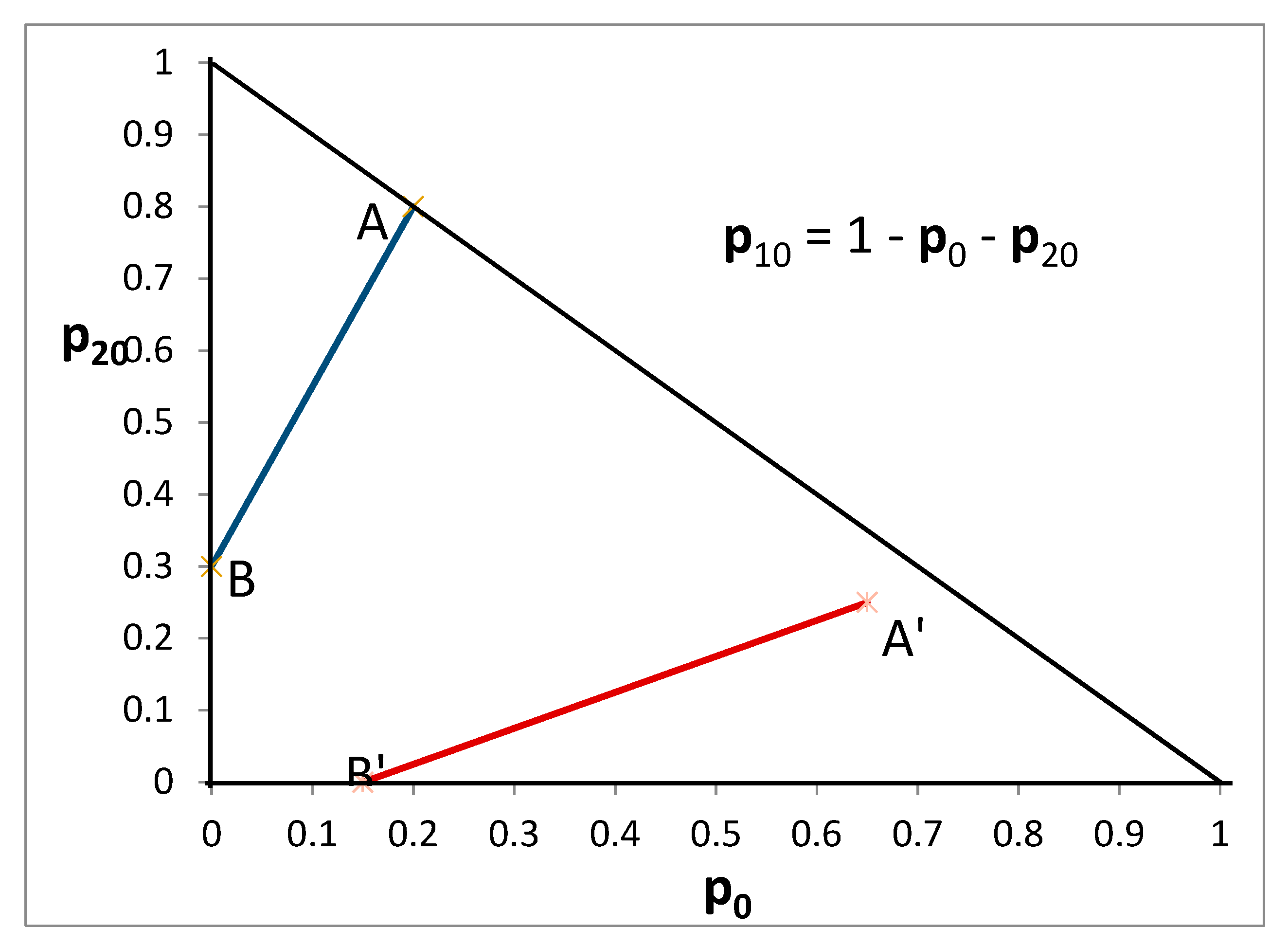
The HO dataset contains 100 unique binary choice tasks.11 Each task was a choice between two lotteries with three prizes drawn from the set {0£, 10£, 20£, 30£}. A crucial design factor was the ratio of (i) the difference between the probability of the high outcome for lottery A and the probability of the high outcome for lottery B to (ii) the difference between the probability of the low outcome for lottery A and the probability of the low outcome for lottery B. It is insightful to represent this choice paradigm in a Machina (1982) [18] triangle, as shown in Figure 1 for the case when the prizes are {0£, 10£, 20£}.
The ratio for the A-B pair is the slope of the line connecting A and B, which is greater than one. The ratio for the A′-B′ pair is the slope of the line connecting A′ and B′, which is clearly less than one. According to EU indifference curves are parallel straight lines with positive slope in this triangle, and the indifference curves of a risk neutral subject would have slope equal to one.12 A wide range of ratios was used in order to identify indifference curves and to test the implications of EU (as well as alternative theories). After all choices were completed, one task was randomly selected and the lottery the subject chose was carried out to determine monetary payoffs.13
One can estimate these parameters for each subject in the HO data set. That approach entails (3 × 80 = 240) parameters, even without the corresponding variance-covariance matrices. Table 1 gives the population mean and standard deviation of the point estimates.14 The last column “LL” gives the sum of the individually maximized log-likelihood values. Note that there is substantial heterogeneity across subjects in the parameter estimates for ρ and β.
These comparisons involve estimates of a large number of parameters. For each individual subject, we obtain point estimates of the parameters, but no confidence interval. One could use a bootstrap procedure to obtain variance-covariance matrices for each individual, but that would be a computationally intense task and entail six additional parameters per subject. Further, the estimates for each subject would ignore the fact that the subjects are random draws from of a population of potential subjects and that therefore the behavior of the other subjects contains information that is relevant to each subject. In contrast, the Bayesian approach is better suited to extract information from the whole sample population. Consequently, we now turn to the Bayesian approach.16
5. Implementing Our Bayesian Approach
When implementing our Bayesian approach we specify the prior g0 as follows. For the logit precision parameter, we specify γ = 20ln[p/(1 − p)] with p uniform on [0.5, 0.999]. In this formulation, p can be interpreted as the probability an option with a 5% greater value will be chosen. Since the mean payoff difference between lottery pairs in the HO data set is about 5%, this is a reasonable scaling factor.17 ρ is uniform on [−1, 1], and ln(β) is uniform on [−ln(3), ln(3)].18 These three distributions are assumed to be independent. For computations, we use a grid of 41 × 41 × 41 = 68,921 points.
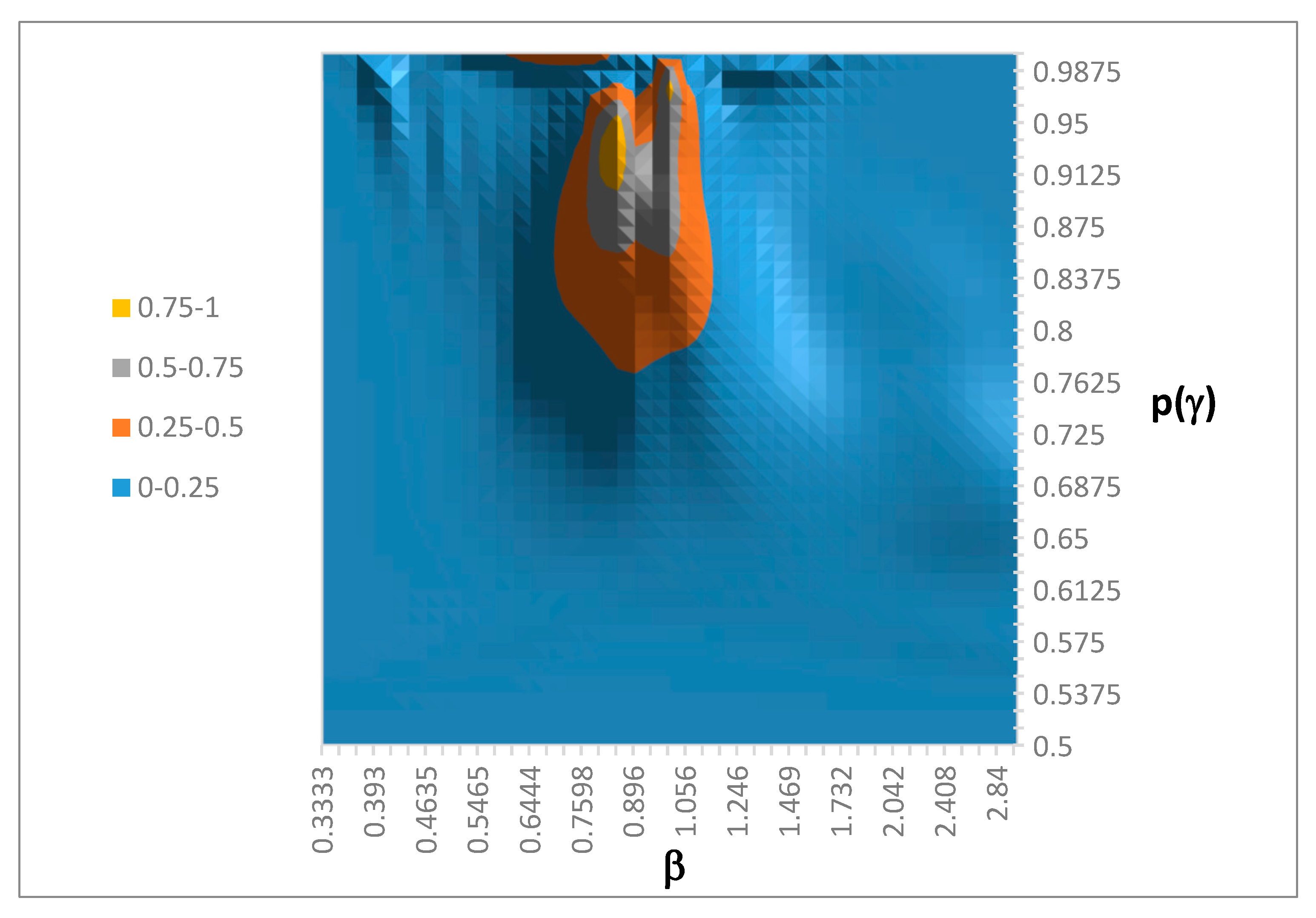
Since we cannot display a three-dimensional distribution, we present two two-dimensional marginal distributions. Figure 2 shows the marginal on (p(γ), β). From Figure 2 we see that the distribution is concentrated around β = 0.95, and that the precision values are large enough to imply that a 5% difference in value is behaviorally significant (i.e., p(γ) > 0.75).
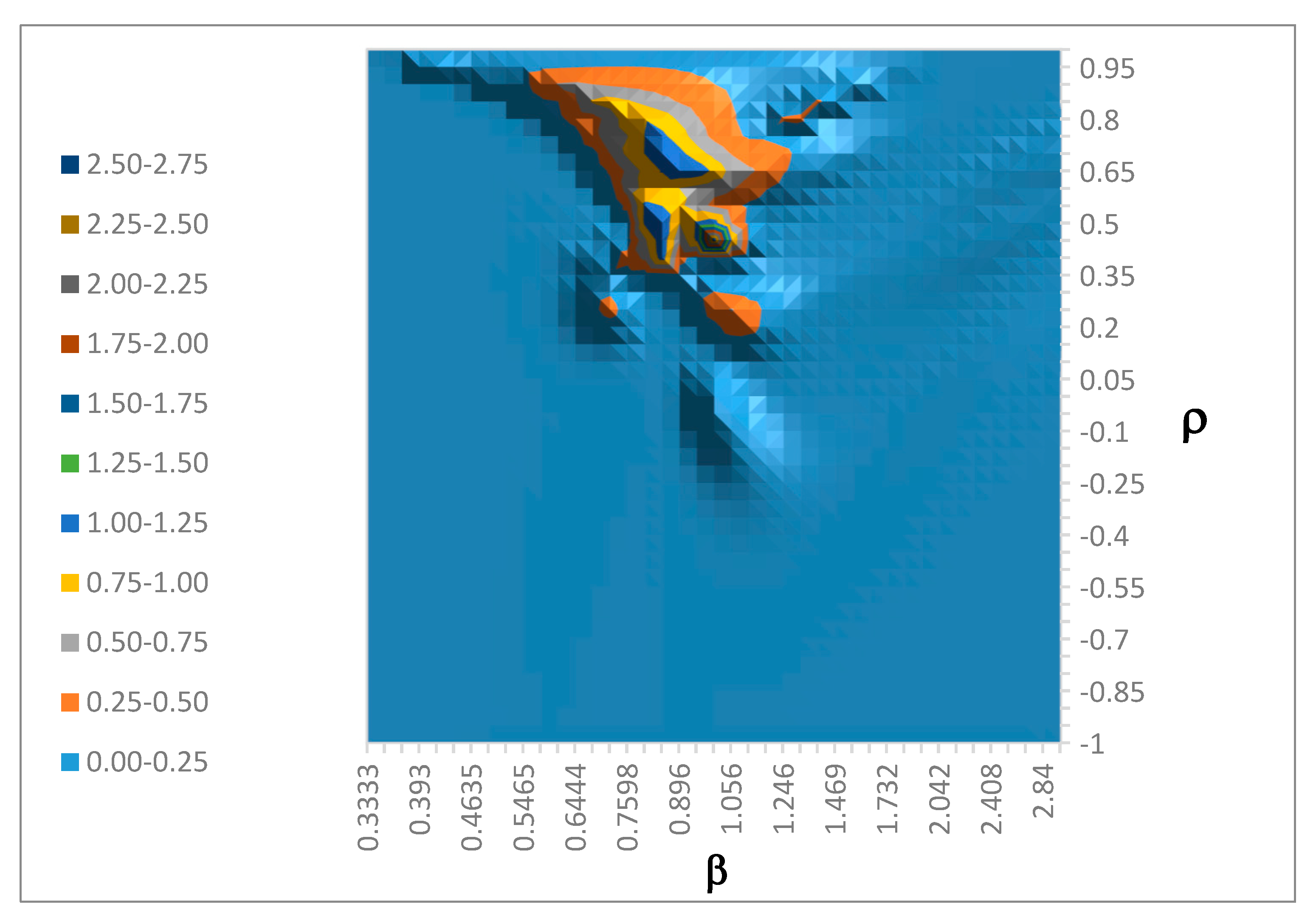
Figure 3 shows the marginal on (ρ, β).
Given g*(θ | x) we can compute several statistics. First, the log-likelihood of the HO data is LL(g*) = −3335.29. In contrast, the log-likelihood of the three-parameter RDEU representative-agent model is −4472.85. Obviously, the heterogeneity implicit in g* fits the data much better than a representative-agent model.19 Compared to −3007.38 (Table 1), the log-likelihood from the Bayesian method appears to be much worse. However, the direct comparison is inappropriate. LL(g*) is computed as if each subject were drawn independently from g*. In contrast, −3007.38 is the sum of individually computed log-likelihoods using the subject-specific estimated parameters.
The g*-weighted mean of the parameter space is = (0.8556, 0.5815, 1.010). Note that ≈ 1, meaning that on average H(F) is the identity function. Table 2 displays the variance-covariance matrix.
However, these means and covariances are much less informative when g* is multimodal.
Indeed, we find evidence for multiple modes. A grid point θ is declared a mode if and only if it has the highest value of g* in a 7 × 7 × 7 cube of nearest neighbors of θ in the grid. The most prominent mode is at p(γ) = 0.999, ρ = 0.85, and β = 0.681. The next most prominent mode is at p(γ) = 0.975, ρ = 0.45, and β = 1.00. The third most prominent mode is at p(γ) = 0.999, ρ = 0.85, and β = 1.47. Numerous other modes exist but are best described as shallow bumps.
Maximum likelihood values are non-decreasing in the number of model parameters, but the additional parameters could be fitting noise, in which case forecasting using a parameter intensive model may be unreliable due to the unobservable noise in the future; this is called over-fitting. To test for over-fitting, we compute g* based only on the first 50 tasks in the HO data, and use this g* to predict the behavior for the second 50 tasks. We find that the log-likelihood of the latter is −1567.39. In contrast, using individual parameter estimates from just the first 50 tasks, the log-likelihood of the second 50 tasks is −1774.01. This result suggests that the approach of individual parameter estimates is more susceptible to over-fitting and less reliable than the Bayesian approach.
6. Behaviorally Distinguishable Parameter Vectors
6.1. Definition
The most productive use of g*(θ | x) is to test hypotheses. For example, we can ask what percent of the subject pool has β = 1. The answer is 10.4%; however, this number is an artifact of the discrete grid used for computation. Assuming g* is absolutely continuous, as the grid becomes finer and finer, we would expect the percentage with β = 1 to approach zero. On the other hand, β = 0.999 is not meaningfully different. What we want to know is the percentage of the population that is behaviorally indistinguishable in some sense from EU (i.e., β = 1).
The behavior is simply the choice data for a random subject xi. To assess whether this data was generated by θ or θ′, we typically compute the log of the likelihood ratio (LLR): ln[f(xi | θ)/f(xi | θ′)]. A positive LLR means xi is more likely to have been generated by θ than θ′. However, it is well-known that likelihood-ratio tests are subject to type-I and type-II errors. To compute the expected frequency of these errors, let X1 ≡ {xi | ln[f(xi | θ)/f(xi | θ′)] < 0}. If the data in fact was generated by θ and xi ∈ X1, then a test of LLR > 0 would yield a type-I error. Similarly, if the data in fact was generated by θ′ and xi ∈ X2 (the complement of X1), then a test of LLR < 0 would yield a type-II error. Hence, the expected frequencies of type-I and type-II errors are respectively:
er1 ≡ ∫X1 f(xi | θ)dxi and er2 ≡ ∫X2 f(xi | θ′)dxi
If either of these error rates is too large, we would say that θ and θ′ are behaviorally indistinguishable. Classical statistics suggests that a proper test statistic would have these error rates not exceed 5%; to be conservative we will use 10% as our threshold.20
Of course, by increasing the number of observations in xi, we can drive these error rates lower and lower. However, practical considerations often limit the number of observations. In laboratory experiments, boredom, time limitations and budget constraints place severe upper bounds on the number of observations. The HO dataset with 100 tasks is unusually large.21 Moreover, to test for overfitting22 we would select a subset, say 50, to use for estimation, and the remaining 50 to assess parameter stability and prediction performance. We believe that 50 distinct choice tasks are a reasonable benchmark because such an experiment will have a duration of about one hour beyond which fatigue sets in. Therefore, for the illustrative purposes of this paper, we use 50 as the sample size upon which to judge behavioral distinguishability.
With 50 binary choices, there are 250 (≈ 1030) possible xi vectors. Generating all these possible xi vectors and computing er1 and er2 is obviously not feasible. Instead, we generate 1000 xi vectors from f(xi | θ) and 1000 from f(xi | θ′).23 Then, er1 is approximated by the proportion of xi generated by f(xi | θ) that lie in X1, and er2 is approximated by the proportion of xi generated by f(xi | θ′) that lie in X2. To ensure robustness to the selection of 50 tasks we randomly selected 25 sets of 50 HO tasks and we averaged max{er1, er2} over these 25 sets of 50 tasks to determine behavioral distinguishability for each (θ, θ′) of interest (see next subsection).
In summary, we define θ and θ′ to be behaviorally distinguishable if both of the simulated type-I and type-II error rates are less than or equal to 10%, and to be behaviorally indistinguishable otherwise.
6.2. Application to RDEU Model and HO Data
Many questions of interest can be framed in terms of our behaviorally indistinguishable relationship on the parameters. To begin, we may want to know what percent of the population is behaviorally indistinguishable from 50:50 random choices (hereafter referred to as Level-0 behavior). Since the latter entails the simple restriction that γ = 0, we can compute whether θ = (γ, ρ, β) is behaviorally distinguishable from (0, ρ, β), and then sum g*(γ, ρ, β) over all the grid points (γ, β, ρ) that are behaviorally distinguishable from (0, ρ, β). The answer is 99.0% (0.5%), which leaves only 1.0% that are behaviorally indistinguishable from Level-0.
The question of most interest is what percent are behaviorally indistinguishable from EU. To answer this, we ask how much mass g* puts on the set of parameters (γ, ρ, β) that are behaviorally distinguishable from Level-0 but indistinguishable from (γ, ρ, 1)? The answer is 79.0% (1.7%). The remainder (99.0 − 79.0) = 20.0% are RDEU types that are behaviorally distinguishable from Level-0 and EU types.
6.3. Comparison with the CHM Mixture Model Approach
This conclusion stands in stark contrast to that of CHM who report 20% EU types and 80% RDEU types. Such a discrepancy requires an explanation. Since CHM used a mixture model, while we used a Bayesian approach, perhaps the different econometric method is the underlying cause of the discrepancy.
To investigate this possibility, we applied our method for measuring the probability mass that is behaviorally indistinguishable from EU (i.e., β = 1) to the CHM mixture model on the same data set [9] (Hey (2001); hereafter H01). That mixture model consists of two types: An RDEU type exactly similar to our specification, and an EU type (RDEU with β restricted to be exactly one). Using the exact same mixture model and parameter estimates as reported in CHM, we computed the implied probability distribution over the RDEU parameters, call it ϕRDEU(ρ, β).24 We find that ϕRDEU puts 0.877 probability mass on parameters (ρ, β) that are behaviorally indistinguishable from EU. The CHM mixture coefficient for the EU type is 0.197, implying that 80.3% are RDEU types. Therefore, we have (0.877*80.3% + 19.7%) = 90.1% of the population that are behaviorally indistinguishable from EU. Thus, when we ask the same question of the H01 data as we do for the HO data, we find similar answers (90.1% and 79.0%, respectively). In other words, both our Bayesian approach and the CHM mixture model approach applied to the H01 data produce similar answers to the same question: What percentage of the population are behaviorally indistinguishable from EU.
To rule out the possibility that this explanation applies only for the H01 data, we confronted the CHM mixture model with the HO data. We implemented the same mixture model as CHM, and found maximum-likelihood estimates for the parameters. As above, we computed the implied probability distribution over the RDEU parameters. We found that ϕRDEU puts 0.844 probability mass on parameters (ρ, β) that are behaviorally indistinguishable from EU. In addition, the mixture coefficient for the EU type was 0.281, implying that 71.9% are RDEU types. Therefore, we have (0.844*71.9% + 28.1%) = 88.8% that are behaviorally indistinguishable from EU, which is larger than the 79.0% we obtained using the Bayesian method but more alike than the mixture coefficient (28.1%).
Thus, it appears that the discrepancy between our conclusions and that of CHM reflects the difference not in the Bayesian versus mixture model approaches but instead reflects the difference in the questions being asked. We ask what proportion of the population are behaviorally distinguishable from Level-0 but not EU types, while CHM ask what is the MLE of the mixture coefficient for the EU type in a specific parametric mixture model.
A way to understand why these questions are substantively different is to realize that the mixture proportion is just a means of creating a general probability distribution. In principle, there are uncountably many ways to represent a given distribution as a mixture of component distributions. Therefore, a crucial step in estimating a mixture model is the provision of identifying restrictions. Since the RDEU model nests the EU model, we need to specify what region of the parameter space should be identified as the EU region even though those parameters also represent an RDEU model. Surely, just the one-dimensional line in (ρ, β) space with β = 1 is far too narrow, but that is the implicit identifying restriction when interpreting the mixture parameter as the percentage of EU types. However, when we ask what proportion of the population are EU types, we want to know what proportion are behaviorally indistinguishable from EU types, and not what weight is given to the EU component in a mixture of two parametric distributions that represents the population distribution.
7. Conclusions and Discussion
This paper has demonstrated the feasibility and usefulness of Bayesian methods when confronting laboratory data, especially when addressing heterogeneous behavior. Specifically, we have presented a nonparametric25 computationally feasible approach. To extend our approach to models with more parameters, statistical sampling techniques can be employed to tame the curse of dimensionality (e.g. see [21]).
We further defined the concept of behavioral distinguishability as a way to answer questions about what proportion of the population behaves similarly to interesting theory-based types.
To demonstrate our method, we applied it to the RDEU model and the HO dataset on lottery choices. Our Bayesian analysis characterized substantial heterogeneity in the subject population. Moreover, it revealed that 79% of the population is behaviorally distinguishable from Level-0 but indistinguishable from EU behavior.
The difference between this finding and the opposite finding by others is not due to the econometric methods but due to the question being asked, or equivalently to what we mean by a behavioral type. When asking what proportion of the population are EU types, we argue that we typically want to know what proportion are behaviorally indistinguishable from EU behavior rather than what weight is given to the EU type in one of infinitely many specifications of a mixture model. A corollary is that we should be cautious when interpreting the weights of a mixture model.
Funding
This research received no external funding.
Conflicts of Interest
The authors declare no conflict of interest.
Appendix A
CHM assume that absent trembles, the probability of choice A is given by P(A | ν, ρ, β) ≡ Φ{[U(FA; ρ, β) − U(FB; ρ, β)]/ν}, where Φ{ } is the standard normal cumulative distribution. Hence, the empirical RDEU model entails three main parameters: (ν, ρ, β). In addition, CHM assume a multivariate normal distribution on (r, b), where r ≡ ln(1 − ρ) and b ≡ ln(β − 0.2791) with mean (, ) and variance-covariance parameters (σr, σb, σrb) that are estimated. The empirical EU model is similar but with β = 1. Finally, the CHM mixture model assumes that a subject is a RDEU type with probability α and an EU type with probability 1 − α, and draws one parameter vector θ ≡ (ν, ρ, β) from the RDEU (or EU) parameter distribution which is used for all lottery choices.
To generate the empirically implied distribution on (r, b) we created a uniform 41 × 41 grid in which r ranges over [ − 2.5, + 2.5] and b ranges over [ − 3, + 3], where and are the MLEs of CHM and also the midpoint of the grid. We then compute the probability density of the Gaussian distribution (given the CHM variance-covariance parameter estimates) for each point in the grid. Let ϕ(r, b) denote this discretized distribution26, and for ease of translation let g(ρ, β) ≡ ϕ[ln(1 − ρ), ln(β − 0.2791)].
When generating simulated data sets for the purpose of computing the probability of type I and type II errors, we fix the variance parameter ν at the CHM estimate for the RDEU type. To generate a simulated data set, for task t ∈ {1, …, 50} we generate a pseudo-random number zt on [0, 1], and if zt ≤ Pt(A |, ρ, β), the choice is A, otherwise the choice is B. The likelihood of this simulated data is f(x |, ρ, β) = ∏t Pt(xt|, ρ, β) given choice xt ∈ {A, B}. Then, this f(x |, ρ, β) is used to determine type-I and type-II errors in accordance with Equation (1).
To ensure robustness to the tasks used, we randomly selected 25 sets of 50 H01 tasks, and we applied the 10% threshold to the average of max{er1, er2} over these 25 sets of 50 tasks to determine behavioral distinguishability of (ρ, β) versus (ρ, 1).
Since the RDEU model nests the EU model, the question of interest for the CHM mixture model is what percentage of the RDEU type is behaviorally indistinguishable from the EU type. The EU type is nested within the RDEU type as the restriction β = 1. Hence, for each point in our 41 × 41 grid, we compute whether (ρ, β) is behaviorally distinguishable from (ρ, 1). Then, using the estimated g(ρ, β), we sum g(ρ, β) over just the grid points (ρ, β) that are not behaviorally distinguishable from (ρ, 1). To this we add the estimated coefficient for the percentage that are pure EU types.
References
- Conte, A.; Hey, J.; Moffatt, P. Mixture Models of Choice under Risk. J. Econom. 2011, 162, 79–88. [Google Scholar] [CrossRef]
- Fox, J.; Kim, K.; Ryan, S.; Bajari, P. A Simple Estimator for the Distribution of Random Coefficients. Quant. Econ. 2011, 2, 381–418. [Google Scholar] [CrossRef]
- Harrison, G.W.; Rutström, E. Risk Aversion in the Laboratory. In Research in Experimental Economics; Cox, J.C., Harrison, G.W., Eds.; Emerald Group Publishing Limited: Bingley, UK, 2008; Volume 12, pp. 41–196. [Google Scholar]
- Harrison, G.W.; Rutström, E. Expected Utility and Prospect Theory: One Wedding and Decent Funeral. Exp. Econ. 2009, 12, 133–158. [Google Scholar] [CrossRef]
- Hey, J.; Orme, C. Investigating Generalizations of Expected Utility Theory Using Experimental Data. Econometrica 1994, 62, 1291–1326. [Google Scholar] [CrossRef]
- Stahl, D. Heterogeneity of Ambiguity Preferences. Rev. Econ. Stat. 2014, 96, 609–617. [Google Scholar] [CrossRef]
- Wilcox, N. Stochastic models for binary discrete choice under risk: A critical primer and econometric comparison. In Research in Experimental Economics; Cox, J.C., Harrison, G.W., Eds.; Emerald Group Publishing Limited: Bingley, UK, 2008; Volume 12, pp. 197–292. [Google Scholar]
- Wilcox, N. Stochastically more risk averse: A contextual theory of stochastic discrete choice under risk. J. Econom. 2011, 162, 89–104. [Google Scholar] [CrossRef]
- Hey, J. Does Repetition Improve Consistency? Exp. Econ. 2001, 4, 5–54. [Google Scholar] [CrossRef]
- Bolstad, W. Understanding Computational Bayesian Statistics; Wiley, ProQuest Ebook Central: Hoboken, NJ, USA, 2012; Available online: http://0-ebookcentral-proquest-com.brum.beds.ac.uk/lib/utxa/detail.action?docID=698546 (accessed on 30 September 2019).
- Kahneman, D.; Tversky, A. Prospect Theory: An Analysis of Decision under Risk. Econometrica 1979, 47, 263–291. [Google Scholar] [CrossRef]
- Quiggin, J. A Theory of Anticipated Utility. J. Econ. Behav. Organ. 1982, 3, 323–343. [Google Scholar] [CrossRef]
- Quiggin, J. Generalized Expected Utility Theory: The Rank-Dependent Model; Kluwer Academic Publishers: Dordrecht, The Netherlands, 1993. [Google Scholar]
- Tversky, A.; Kahneman, D. Cumulative Prospect Theory: An Analysis of Decision Under Uncertainty. J. Risk Uncertain. 1992, 5, 297–323. [Google Scholar] [CrossRef]
- Prelec, D. The Probability Weighting Function. Econometrica 1998, 66, 497–527. [Google Scholar] [CrossRef]
- Stahl, D. Assessing the Forecast Performance of Models of Choice. J. Behav. Exp. Econ. 2018, 73, 86–92. [Google Scholar] [CrossRef]
- Harrison, G.W.; Swarthout, J.T. Experimental Payment Protocols and the Bipolar Behaviorist. Theory Decis. 2014, 77, 423–438. [Google Scholar] [CrossRef]
- Machina, M. Non-expected Utility Theory. In The New Palgrave Dictionary of Economics, 2nd ed.; Durlauf, S.N., Blume, L.E., Eds.; Palgrave Macmillan: Basingstoke, UK, 2008. [Google Scholar]
- Loomes, G.; Sugden, R. Testing Alternative Stochastic Specifications for Risky Choice. Economica 1998, 65, 581–598. [Google Scholar] [CrossRef]
- Bruhin, A.; Fehr-Duda, H.; Epper, T. Risk and Rationality: Uncovering Heterogeneity in Probability Distortion. Econometrica 2010, 78, 1375–1412. [Google Scholar] [CrossRef]
- Rubinstein, B.; Kroese, D. Simulation and the Monte Carlo Method, 3rd ed.; Wiley & Sons: Hoboken, NJ, USA, 2016. [Google Scholar]
| 1 | |
| 2 | In Section 2 we will comment on why MCMC methods cannot be used to generate samples from g*. |
| 3 | Similar analysis was done on the data of [9] and similar results were obtained. |
| 4 | Note that almost all the volume of such a high dimensional simplex is very near the boundaries, so a uniform prior would put essentially zero probability on interior points. Therefore, the amount of data and time for Bayesian updating to converge is likely to be longer than the lifetime of the Milky Way galaxy. |
| 5 | The variance-covariance matrix in four dimensions has 10 degrees of freedom subject also to being positive semi-definite. |
| 6 | The mixture over K modes entails K − 1 mixture parameters, so there are 14K + K − 1 = 15K − 1 dimensions of G. The variance-covariance matrix in 15K − 1 dimensions has (15K − 1)15K/2 = (225K2 − 15K)/2 free parameters. |
| 7 | The number of variance-covariance parameters could be drastically reduced by assuming zero covariance and even symmetry, but at the potential cost of serious mis-specification. |
| 8 | This model is the same as the Cumulative Prospect model [11] restricted to non-negative monetary outcomes. |
| 9 | Alternative specifications are (i) symmetric Quiggin [12], and (ii) Prelec [15]. However, the effect of alternative specifications of H( ) is orthogonal to the purpose of this paper, which is the econometric method. For evidence that our results would be the same under the Prelec [15] specification, see [16]. |
| 10 | As pointed out by [17], this specification implicitly assumes the “compound independence axiom”. Since we view EU and RDEU as behavioral models, we are comfortable with this implicit assumption. |
| 11 | These 100 tasks were presented to the same subjects again one week later. We do not consider that data here because the test that the same model parameters that best fit the first 100 choices are the same as those that best fit the second 100 choices fails. Possible explanations for this finding are (i) that learning took place between the sessions, (ii) preferences changed due to a change in external (and unobserved) circumstances, and (iii) the subjects did not have stable preferences over this time period. Therefore, we focus our attention on the first 100 choice tasks. |
| 12 | A risk neutral decision maker would be indifferent between lottery A and B if and only if both yield the same expected monetary value. Letting H denote the high prize, M the middle prize and L the low prize for a pair of lotteries, equating expected utility yields that the slope ≡ (pAH − pBH)/(pAL − pBL) = (H − M)/(M − L), which in Figure 1 is identically one. For other lottery pairs in the HO experiment, the slope of risk neutral indifference can be 0.5, one, or two. |
| 13 | Loomes and Sugden [19] is a similar study as [5]), except that their analysis of the data is based on non-parametric tests involving the number of “reversals” and violations of dominance. Hey [9] reports a similar study with 100 binary tasks repeated over five days. Harrison and Rutström [4] replicate HO and also run a similar experiment using 30 unique tasks. Bruhin et al. [20] also explore heterogeneity, but they elicit certainty equivalents, so the task is arguably different from binary choices as in the other studies. |
| 14 | This is the square root of the variance of the point estimates across subjects; it is not the standard error of individual point estimates. |
| 15 | Note that p(γ) is the probability the subject will choose the option with the greater value whenever that value is 5% higher than that of the other option, thereby providing a behavioral interpretation of γ. |
| 16 | For another application, see [6]. |
| 17 | Our results are robust to this specification of the prior on γ. |
| 18 | 95% of the individual MLEs for β lie in this range. Using a wider interval for the prior on β has no noticeable effect on the Bayesian posterior at the cost of more grid points and computational time. |
| 19 | One can consider this Bayesian approach as an alternative random parameter model as used by [7]. However, in contrast to Wilcox, we assume that each subject draws from this distribution once and uses those parameters for all choice tasks, rather than drawing for each choice task. |
| 20 | Note that setting limits on these error rates is similar to setting lower and upper test thresholds on LLR. |
| 21 | See footnote 12. |
| 22 | On the dangers of overfitting see [16]. |
| 23 | We also made these computations with only 100 simulated xi vectors, and found virtually the same results. Therefore, we are confident that 1000 simulated xi vectors are adequate for our purposes. |
| 24 | See Appendix A for details. Note that this distribution is an estimate of the population distribution of parameter values, and so comparable to the Bayesian estimate g*. Since the CHM mixture model is bimodal, while our Bayesian estimate revealed three prominent modes, the estimated distributions are obviously different. However, it could still be the case that the probability masses for a specific subset of parameter values turn out to be similar. |
| 25 | That is, the Bayesian posterior is a non-parametric function of the data, albeit the RDEU model is obviously parametric. |
| 26 | Since we use a bounded range for these parameters, it is important to verify that we are not excluding a non-negligible probability mass. To do so, we simply sum ϕ(r, b) over our grid. The result is 99.9996%. |
Figure 1.
Example of lottery choice pairs.

Figure 2.
Marginal of g* on (p(γ), β).

Figure 3.
Marginal of g* on (ρ, β).


Table 1.
Population mean and standard deviation of individual parameter estimates and the aggregated Log-likelihood(LL), Equation (12).
Table 1.
Population mean and standard deviation of individual parameter estimates and the aggregated Log-likelihood(LL), Equation (12).
| p(γ) a | ρ | Β | LL |
|---|---|---|---|
| 0.8826 (0.0921) | 0.4465 (0.4405) | 1.028 (0.637) | - 3007.38 |
a p(γ) ≡ 1/[1 + exp(−0.05γ)].15
Table 2.
Variance-covariance of g*.
| p(γ) | ρ | Β | |
|---|---|---|---|
| p(γ) | 0.0085 | −0.0054 | −0.0150 |
| ρ | 0.0851 | 0.0335 | |
| β | 0.1638 |
© 2019 by the author. Licensee MDPI, Basel, Switzerland. This article is an open access article distributed under the terms and conditions of the Creative Commons Attribution (CC BY) license (http://creativecommons.org/licenses/by/4.0/).
Share and Cite
MDPI and ACS Style
Stahl, D.O. A Bayesian Method for Characterizing Population Heterogeneity. Games 2019, 10, 40. https://0-doi-org.brum.beds.ac.uk/10.3390/g10040040
AMA Style
Stahl DO. A Bayesian Method for Characterizing Population Heterogeneity. Games. 2019; 10(4):40. https://0-doi-org.brum.beds.ac.uk/10.3390/g10040040
Chicago/Turabian StyleStahl, Dale O. 2019. "A Bayesian Method for Characterizing Population Heterogeneity" Games 10, no. 4: 40. https://0-doi-org.brum.beds.ac.uk/10.3390/g10040040
Note that from the first issue of 2016, this journal uses article numbers instead of page numbers. See further details here.