Taxation with Mobile High-Income Agents: Experimental Evidence on Tax Compliance and Equity Perceptions


1
Department of Economics and Management, University of Trento, via Inama 5, 38122 Trento, Italy
2
Department of Economics, University of Erlangen-Nuremberg, Lange Gasse 20, 90403 Nürnberg, Germany
*
Author to whom correspondence should be addressed.
Games 2019, 10(4), 42; https://0-doi-org.brum.beds.ac.uk/10.3390/g10040042
Submission received: 9 September 2019
/
Revised: 1 October 2019
/
Accepted: 4 October 2019
/
Published: 11 October 2019
(This article belongs to the Special Issue Empirical Tax Research and Application)
Abstract
:In a laboratory experiment on tax compliance, we model a situation in which high-income taxpayers can leave a tax system that finances a public good. We compare low-income taxpayers’ compliance decisions and equity perceptions across treatments in which they are informed or not informed about the mobility option of high-income taxpayers. This allows us to test if low-income taxpayers regard the mobility option as a rationale for implementing a regressive tax schedule. To investigate if a potential ‘justification effect’ of the mobility option depends on the causes of income heterogeneity, we also varied whether income was allocated based on relative performance in a prior ability task or at random. Interestingly, although the performance-based allocation itself was judged to be fairer, we observed higher compliance under the random allocation mechanism. However, compliance and equity perceptions did not significantly differ by the information treatment variation, regardless of the source of income inequality. The results indicate that the threat of losing high-income taxpayers’ contributions does not lead low-income taxpayers to view the regressive tax schedule more favorably. This suggests that taking the differential mobility options as given and altering tax schedules accordingly may not be perceived as an adequate policy response.
Keywords:
tax compliance; mobility; heterogeneous income; optimal taxation; fairness perceptions; laboratory experimentJEL Classification:
C91; H261. Introduction
In a world in which high-income taxpayers are more responsive to taxation than low-income taxpayers, governments are compelled to lower taxes on high-income taxpayers compared to what would otherwise be seen as a socially desirable tax schedule. One response margin that may underlie ‘higher responsiveness’ is actual relocation of the taxpayer to a different jurisdiction. While mobility for labor is typically not as high as for capital, there is evidence that individual mobility increases with skill [1] and is sensitive to tax rates [2], especially for top professionals [3,4]. Countries may then perceive competitive pressures to attract or retain mobile high-income individuals and effectively be compelled to lower taxes on them [5,6]. Denmark, for example, offers new immigrants with high income a preferential tax rate of nearly half the rate for domestic workers, a scheme which [7] found to be very effective at attracting highly paid workers. According to an OECD report from 2011, 15 other OECD countries had introduced tax concessions for high-skilled workers. Although ‘obvious’ tax concessions are often confined to foreigners, similar competitive pressures exist for domestic high-income taxpayers. As [8] write in their survey article on international tax competition, ‘the reduction in top marginal rates of personal taxation (…) [is] reflecting the mobility of high earners and (…) tax avoidance opportunities (…)’.
At the same time, a widely held normative belief is that those who can afford to carry a higher share of the tax burden should do so.1 Such equity principles may be in conflict with the logic of lowering taxes on mobile high-income taxpayers. The OECD report, for instance, states that ‘tax concessions will create equity concerns by treating differently high-skilled and less-skilled workers’ ([9], p. 124).2 Equity perceptions, in turn, are believed to influence tax compliance [10,11], raising the possibility that compliance is adversely affected by a preferential tax treatment of high-income taxpayers. In what follows, we generically refer to the possibility of legally avoiding taxation (e.g., by relocating abroad) as ‘outside option’.3 Because reliable information on tax compliance and equity perceptions is difficult to obtain simultaneously with exogenous variation in outside options, we conducted a laboratory experiment.
In this experiment, we focus on a closely related situation. In our set-up, high-income taxpayers are offered a preferential tax rate so that they do not leave the ‘domestic’ tax system. We investigate if low-income taxpayers’ equity perceptions and compliance behavior are susceptible to the logic of offering high-income taxpayers preferential tax treatment because of their outside options. We are particularly interested in this situation because it may create a conflict of interest among low income-taxpayers who are better off if the high-income taxpayers do not opt out but may resent the preferential tax rate. Thus, we compare the tax compliance and tax equity perceptions of experimental participants with low income and high tax rates across conditions in which they do or do not know about an outside option for participants with high income and a low tax rate.4 Because we suspected that a potential ‘justification effect’ of an outside option might depend on the perceived equity of the initial income inequality, we conducted this treatment comparison under two different allocation conditions: one in which high and low incomes were allocated at random and one in which they were allocated according to relative performance in a prior cognitive ability task, with the latter allocation arguably carrying some connotation of ‘desert’ or ‘merit’.
Our main result is that regardless of the source of income inequality, compliance and perceptions do not react favorably to the exogenously provided reason for preferential tax treatment of high-income taxpayers. In terms of policy, this suggests that governments would find it difficult to increase (but also would not harm) tax compliance by communicating the existence of outside options as rationale for taxing high-income taxpayers at lower rates. It may also be taken to suggest that taking differential outside options as given and altering tax schedules accordingly is not perceived as an adequate policy response. Our second finding shows that random allocation of advantages led to higher tax contributions than the performance-based allocation mechanism. A possible interpretation is that being in the position of a low-income taxpayer through worse cognitive performance is particularly unpleasant and thereby not conducive to cooperative behavior.
The remainder of this chapter is organized as follows. In the next section, we review the literature that the present study relates to. Section 3 explains the experimental design. Section 4 briefly states predictions and hypotheses. The results are presented and discussed in Section 5. The final section concludes.
2. Related Literature
Our study thematically relates to the experimental literature on tax compliance and in particular the nexus between tax compliance and equity perceptions. As we construe taxation and compliance as a cooperative endeavor, it also connects with certain experimental studies of general aspects of other-regarding behavior and cooperation, i.e., studies that are not specifically motivated and framed in the context of taxation. We begin by giving a brief overview of the experimental literature on tax compliance and point out connections to other experimental studies at the end of this section.
The experimental literature on tax compliance owes its existence and breadth largely to the fact that with observational data, tax compliance is difficult to measure and exogenous variation in independent variables of interest can be hard to find (see [14], for an overview of methods to measure tax non-compliance). In contrast, laboratory experiments offer a way to easily measure compliance and induce exogenous variation by design, although at the cost of raising concerns with regards to the external validity of the results.5 Some, in particular earlier studies, have directly implemented simple experimental analogues of Allingham and Sandmo’s [16] influential [1972] model of tax compliance as an individual decision under risk. While some of its main comparative static results—higher audit probabilities and fines increase compliance—have by and large been confirmed (see e.g., [17,18]), several authors have argued that observed levels of compliance are too high to be explained only by aversion to the risk of being fined (e.g., [19,20,21]).6 Partially in response to the debate about the merits and demerits of the Allingham-Sandmo model, partially as independent efforts to understand the determinants of tax compliance, experimental designs have tended to become more involved, introducing inter alia public good elements (e.g., [17,19,23,24]), heterogeneous and earned income [23,25,26], richer tax schedules [26,27,28] or endogenous audit rules [29,30]. Other studies haven taken up psycho-social factors like the role of persuasion [31], moral constraints [32,33] and emotions [33,34], and still others investigated design factors such as the role of framing (e.g., [19,25,35]) or income source [25,36].7 Importantly for the current investigation, several studies found that equity concerns affect the compliance decision [10,11,37]. Interpreting taxation as a cooperative endeavor and non-compliance as free-riding, such influence of equity concerns is reminiscent of ‘conditionally cooperative’ behavior, as it has been observed in public good experiments [38]. We are, however, not aware of a study that addresses the potential equity-mediated interaction between outside options, tax schedules and tax compliance. Our study specifically tests whether an outside option is accepted as a rationale for tax concessions by comparing equity perceptions and compliance behavior across treatments in which participants do and do not know about the existence of this outside option.8 In other words, within the experimental literature on tax compliance, our study appears to be the first to investigate if constraints to more equitable taxation—through their potential effects on equity perceptions—affect compliance behavior. Prima facie evidence for the possibility of such a ‘justification effect’ of constraints that might induce a change in cooperative behavior through a change in perceptions comes from ultimatum game experiments: [39] and [40] report that outside options affected the distribution of offers and rejections by changing the fairness perception of a given offer. Ref. [40], for instance, finds that when responders had an outside option, offers were higher and given offers were also rejected more often. While the tax game of the present study is different from an ultimatum game, the underlying idea in common is that outside options influence how players perceive and evaluate a given situation and that this evaluation could ultimately affect behavior. The next section describes how we implemented this idea in the context of the tax compliance experiment.
3. Experimental Design
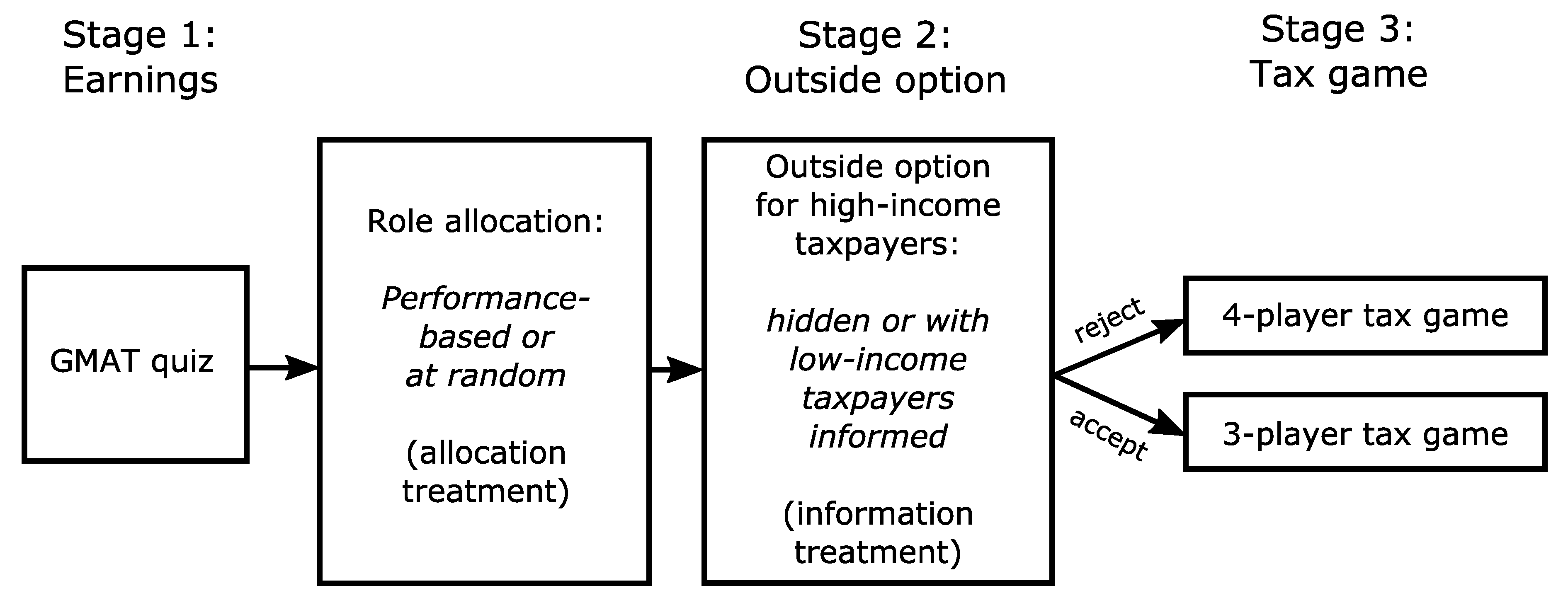
We study the compliance decisions and tax equity perceptions of taxpayers in a laboratory environment with heterogeneous income, differential outside options and a regressive tax schedule. The main dependent variable of interest was compliance behavior of low-income taxpayers in a one-shot multi-player tax game, which we will describe in detail below. One treatment variation lay in the knowledge low-income taxpayers had about the existence of an outside option for high-income taxpayers. The idea behind this treatment variation was to test if knowledge about the outside option leads low-income taxpayers to view a reduced tax rate for high-income taxpayers less negatively and if such ‘justification by constraints’ (i.e., the outside option threat) materializes in higher compliance behavior by low-income taxpayers. Because we suspected that such an effect might depend on the causes of income heterogeneity, we also varied whether roles were allocated based on relative performance or at random. In the first six experimental sessions, a prior cognitive performance contest motivated the allocation of different roles and in particular incomes: high-income taxpayer positions were given to those participants with the highest relative performance in the earnings stage. In the six remaining experimental sessions, role allocation was random (but the earnings stage was retained for comparability).9 Table 1 displays the four treatment conditions that result from the between-subjects combination of outside option information and role allocation mechanism treatments. Figure 1 provides a visual overview of the main stages and features of the experimental design.
We proceed now in chronological manner, explaining first the earnings stage, then an intermediate stage in which the outside option information treatment variation occurred, and then the tax game. All elements except the intermediate stage containing the outside option were explained in the instructions that were read aloud before the experiment started.10 These instructions were using tax language, but were otherwise framed as neutrally as possible.11 The experiment concluded with a questionnaire on tax equity perceptions and risk preferences.
Stage 1: Earnings stage.
Participants had 15 min to answer nine multiple choice questions taken from the Graduate Management Admission Test (GMAT).12 In the performance-based role allocation condition, relative performance on these GMAT questions determined role allocation, with the best-performing participants being granted ‘role A’ (high income) and the remainder being allocated to ‘role B’ (low income).13 In the randomized role allocation condition, role allocation was random and hence independent of GMAT performance. Participants in role A earned 500 experimental points as their initial income in the tax game. Participants in role B earned 100 points. Each participant was privately informed about his or her resulting role on the computer screen immediately after stage 1.
Stage 2: Outside option decision by high-income taxpayers.
After stage 1, participants in role A were given the opportunity to opt out of the succeeding tax game. More precisely, they could either participate in the tax game or take a fixed fraction (95%, i.e., 475 points) of their earned income as final earnings instead. The fraction was chosen such that given the tax rates and compliance rules in the following tax game, it would always be weakly profitable for them not to opt out.14 This ensured that an interpretation that the tax rate was low enough to prevent the flight of high-income taxpayers was independent of beliefs.15 If a participant in role A decided to participate, she would form a group of four players with three participants in role B in the following tax game. If a role A participant opted out instead, the three participants in role B would form a group of three players in the tax game.
The information treatment difference lay in the information that low-income taxpayers were given about the outside option. In treatments with no information, low-income participants were unaware about the existence of the outside option. They had only been instructed that they could be in a group of three low-income taxpayers or a group of three low-income and one high-income taxpayer in the subsequent tax game.16 In treatments with information, low-income taxpayers were informed about the outside option of high-income taxpayers and that the composition of their group depended on the high-income taxpayer’s decision.17
During this stage, all taxpayers had to calculate the minimum and maximum earnings for high-income taxpayers in the tax game explained next. In addition, low-income taxpayers had to calculate the minimum and maximum earnings for high-income taxpayers under a counterfactual tax rate of 50% for both high and low-income taxpayers. While for all participants these questions may have appeared like standard control questions, their purpose was to make it explicit to informed low-income participants that the outside option for high-income taxpayers was not profitable under the given tax rates, but would be under a counterfactual tax schedule with a higher rate on high income. To gain information on whether participants had understood this connection between the tax rate for high-income taxpayers and the outside option, we also asked informed low-income taxpayers about their belief as to whether the high-income taxpayer in their group would opt out, and if they themselves would opt out if they were in the situation of a high-income taxpayer under the given and under the counterfactual tax rate regime.18
Stage 3: Tax game.
In stage 3, the actual tax game interaction, participants’ income from stage 1 was subject to tax. High-income (‘role A’) taxpayers were taxed at rate and low-income (‘role B’) taxpayers at rate . Taxes paid amounted to a public good: collected taxes were multiplied by 2 and shared equally among the members of a group. While group members had the possibility to contribute less than their due amount—namely any integer between 0 and their tax liability of 50 points—paying less entailed the risk of being audited and fined. More precisely, high-income participants were audited with certainty while for low-income participants, the audit probability was 5%. For high-income participants, non-compliance within the tax game was hence not a viable option.19 If audited and found to have contributed less than the due amount, participants had to pay their full tax liability and additionally a fine in the amount of their tax contribution gap.20
As explained above, participants could either be in a group of one high-income and three low-income participants or in a group of three low-income participants only. With denoting pre-audit contributions, an indicator function for the occurrence of an audit, post-audit contributions and group size, the following payoff functions summarize the tax game:
Further details. After the instructions were read out aloud, participants had to answer control questions about payoffs and the rules of the game. Stage 1 began when all participants had answered these correctly. We also asked participants for their beliefs about others’ compliance decisions.21
The experiment was computerized using z-Tree [42] and conducted at the Laboratory for Experimental Research at the University of Erlangen-Nuremberg. Participants were recruited from the laboratory’s student participant pool using ORSEE [43]. In total, 348 students participated in 12 sessions.22 Participants were paid a show-up fee of 4 Euro, plus the points from the experiment, converted at a rate of 25 experimental points = 1 Euro. On average, participants earned 12.75 Euro for a session of 65 min. Experimental sessions were run between May and November 2015. Table 2 shows that while the average earnings for different session types were very similar, participants in role A (high-income taxpayers) earned substantially more than participants in role B (low-income taxpayers): across all sessions, the mean earnings were 24.46 Euro for high-income taxpayers and 9.38 Euro for low-income taxpayers respectively.
4. Predictions
It can easily be verified that low-income taxpayers maximize their expected payoff by contributing zero and high-income taxpayers by contributing in full.23 Furthermore, given the low enforcement threats for low-income taxpayers, risk aversion is an unlikely explanation for positive compliance levels.24 In other words: a standard expected utility model of behavior would predict zero tax contributions for low-income taxpayers. Conversely, observed positive tax compliance choices can be interpreted to reveal preferences over ‘something else’ than the financial stakes involved for the decision-maker herself—where ‘something else’ could be anything from social preferences along the lines of [44] to a perceived ‘duty-to-comply’ in taxation contexts [45] or with social norms more generally. Furthermore, it is worth noting that because the financial incentives are the same for informed and uninformed taxpayers, any model of utility based purely on financial outcomes (including outcome-based social preference models) predicts no treatment difference with regards to information. Alternatively, if compliance depends on equity perceptions and the low tax rate for high-income taxpayers is seen as more acceptable when ‘justified’ by the outside option, one would expect more contributions in the treatment conditions with information. Because we conjectured the performance-based allocation to be viewed as more fair than the random type allocation, we expected less of a ‘justification effect’ of information in the treatments with performance-based allocation compared to the effect in the random allocation conditions.25 We state these two predictions with regards to the role of information about the outside option as hypotheses:
Hypothesis 1 (Justification effect):
Compliance of low-income taxpayers in groups of four is higher when they are informed about the outside option of high-income taxpayers.
Hypothesis 2 (Justification effect interaction with allocation type):
The justification effect is smaller in treatments with performance-based allocation of taxpayer types (compared to treatments with random allocation).
5. Results
Before the analysis of compliance choices and equity perceptions, we first establish that participants understood the basic incentive structure of the experiment. We then analyze the effect of the information and the allocation treatment dimension on compliance choices. The lack of a positive effect of information about the outside option on compliance and the negative effect of performance-based allocation are then further interpreted in light of the stated equity perceptions and tax preferences.
5.1. Manipulation Checks
Over 90% of high-income taxpayers (72 out of 78) chose the weakly dominant strategy of not opting out and then contributing fully in the tax game interaction.26 More than 80% of informed low-income taxpayers (93 out of 114) stated the corresponding rational belief that high-income taxpayers would in fact not take their outside option. Moreover, over 70% of informed low-income taxpayers (81 out of 114) also stated they would not opt out themselves if they were in the position of a high-income taxpayers under the prevailing tax structure, but would do so under a counterfactual tax rate of 50% for high-income taxpayers. Hence most participants seemed to understand the basic incentive structure of the experiment; in particular the majority of informed participants understood that the outside option was not financially attractive for high-income taxpayers under the prevailing tax scheme, but would become attractive if the tax rate on high-income taxpayers were as high as the factual tax rate for low-income taxpayers. The subsequent results on compliance choices are qualitatively robust to excluding the participants who, based on their stated beliefs and intentions, appear to have been ‘confused’ about the incentive structure.27
5.2. Compliance Choices and Treatment Effects
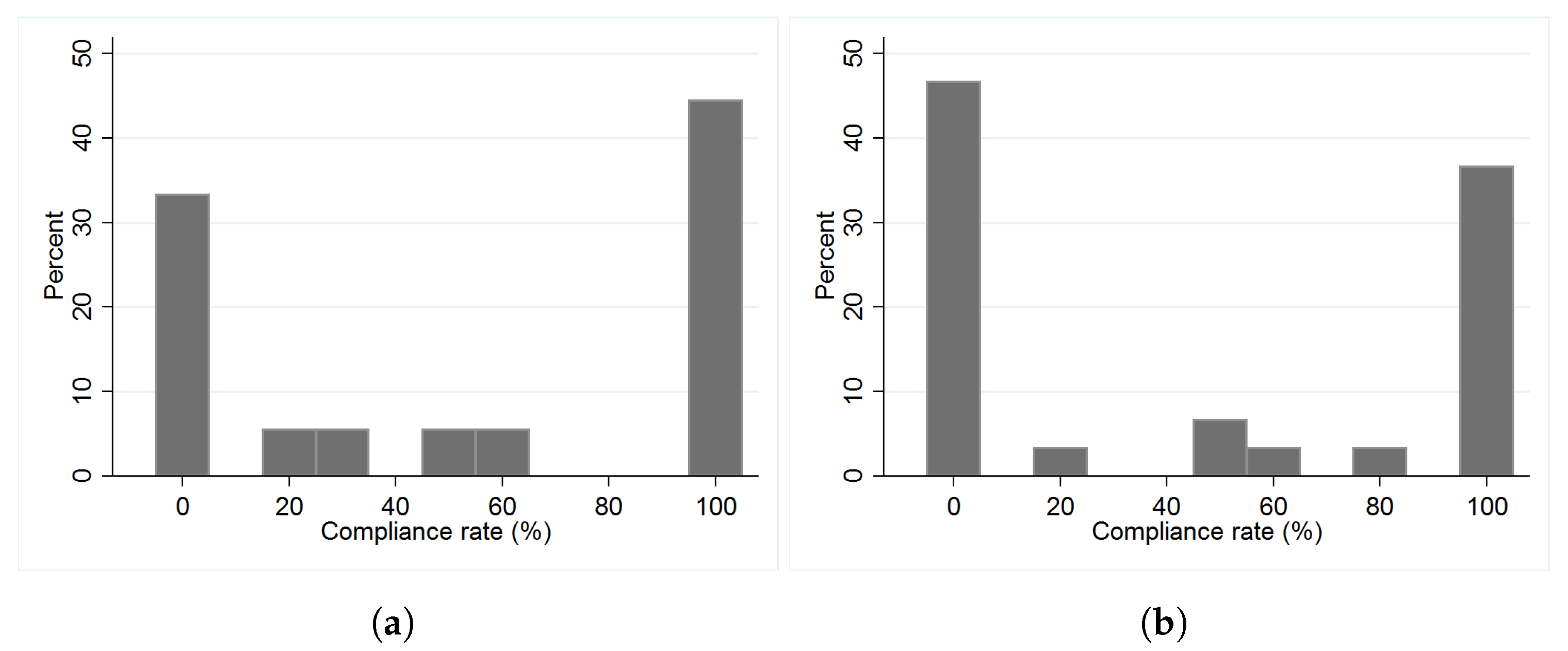
We now proceed to analyzing compliance choices, focusing on the compliance choices of low-income taxpayers in groups of four.28 Figure 2 plots the corresponding distributions of compliance rates by treatment.29
We briefly take note that across all treatments, a majority of low-income taxpayers (62%) chose positive contribution levels, i.e., did not make an expected payoff-maximizing choice. This suggests that their compliance choices were not exclusively guided by financial considerations.30 This is also consistent with the fact that contributions strongly correlate with stated beliefs about others’ contributions (see Appendix A Table A3, Table A4, Table A13 and Table A14), in line with the public goods structure of the tax game and prior evidence of ‘conditionally cooperative behavior’ in such situations [38]. We also note that compliance choices were concentrated at the boundaries of zero and full compliance.31 This bipolar distribution of compliance rates is consistent with prior experimental evidence and available field data on compliance rates for taxpayers with self-reported income [15].
The compliance choice distributions displayed in Figure 2 reveal that there is no indication at all that being informed about the outside option increased compliance levels. Table 3 shows the corresponding statistical results of OLS regressions of compliance choices on the treatment indicator for information.32 Whether collapsing the two allocation conditions or analyzing them separately: the coefficient on the information treatment indicator does not even come close to reaching a 10-percent significance level (and in case of the performance-based allocation, its sign is even negative).33 This pattern does not change if ‘confused’ participants are excluded from the analysis (see columns (4)–(6) in Table 3). The results are also qualitatively robust to adding stated risk preferences, beliefs about others’ contributions and GMAT performance as covariates to the regressions (see Table A3 and Table A4 in the Appendix A). Moreover, the coefficient on the information treatment indicator is also not significantly different between performance-based and random role allocation (see Table A10 and Table A11 in the Appendix A). If the true effect of being aware of the outside option is indeed negative and small as in the data, many more observations would be needed to ‘confirm’ this statistically (i.e., reach conventional statistical significance).34 Bayesian updating of the prior probability of Hypothesis 1 lead us to believe that this does likely not hold given the data observed. We essentially conclude that the true effect must be small and may even be negative.
Looking at participants’ post-experimentally stated equity perceptions (Figure 3), we note that awareness of the outside option did not affect these perceptions. In particular, whether knowledgeable about the outside option or not, low-income taxpayers rated the tax schedule as equally unfair and the lower tax rate for high-income taxpayers as not justified.35 Moreover, informed low-income taxpayers expressed a preference for non-regressive tax rates in spite of the outside option, for increasing the tax rate for high-income taxpayers, and limited agreement to a statement that the risk of the high-income taxpayers opting out ‘justifies’ the lower tax rate (see Table A5 in the Appendix A).36 The hypotheses that the existence of an outside option might provide a compliance-enhancing ‘justification’ for the low tax rate on high-income taxpayers (Hypothesis 1) and that this effect would be larger in treatments with performance-based allocation (Hypothesis 2) are therefore not confirmed in the experimental set-up and data.
Result 1 (Irrelevance of outside option):
Being informed about the outside option of high-income taxpayers did not affect low-income taxpayers’ compliance choices nor their expressed equity perceptions.
The distributions displayed in Figure 2 do suggest, however, that compliance is higher when player types are allocated randomly rather than based on relative performance. In fact, this visual impression bears out in nonparametric and parametric statistical tests. Table 4 presents the results of OLS regressions of compliance rates on an indicator for performance-based player type allocation, with and without controlling for performance in the earnings stage itself. Compliance rates are significantly lower under the performance-based player type allocation.37 Restricting the analysis to participants who do not exhibit signs of confusion yields very similar results (see Table A7). The overall difference appears to stem chiefly from informed taxpayers, but the coefficient on the performance-based allocation indicator is not significantly different between informed and uninformed taxpayers (see Table A10 and Table A11 in the Appendix A).
It should be noted that by construction, the composition of low-income taxpayers differs between random and performance-based allocation treatments in terms of their performance on the GMAT questions in the earnings stage. Because performance in the earnings stage itself is negatively correlated with compliance (see Table A12) and performance-based allocation treatments have worse-performing low-income taxpayers than random allocation treatments by construction (, Mann-Whitney U test), it is unsurprising that the allocation type effects become somewhat larger when GMAT scores from the earnings stage are added as a covariate to the regressions. The results are also qualitatively robust to the inclusion of further covariates such as stated risk preferences (Table A13 and Table A14). We therefore conclude that the random allocation of taxpayer types increased compliance compared to the performance-based mechanism.
Result 2 (Main effect of allocation type):
Compliance levels were higher in treatment conditions with random rather than performance-based allocation of taxpayer types.
This occurred despite the fact that participants (including low-income participant) judged the performance-based mechanism to be fairer than random allocation in the post-experimental questionnaire, consistent with the meritocratic element of performance-based allocation.38 If compliance behavior is positively influenced by fairness perceptions, this would raise the question why contributions were not lower in the random allocation. One plausible interpretation is that the competitive element of our performance-based allocation treatment reduced participants’ pro-social orientation.39 Such an explanation appears consistent with studies on giving behavior [53,54,55]. Ref. [53] found that providing information about relative ability decreased the amount of giving to unknown recipients.40 Ref. [54], in turn, documented that participants gave more to third-parties when their income was uniform and independent of prior absolute performance on GMAT questions, with the difference stemming from the ‘increased generosity of low performers’ under the ‘egalitarian’ vis-à-vis the ‘meritocratic’ treatment.41 While in the first study by Riyanto and Zhang the difference in pro-social behavior appears to be driven exclusively by social comparisons of ability, in the second study it apparently stemmed from the different allocation rules themselves. We also note that negative feedback about one’s relative performance on a cognitive ability task (rather than ‘pure’ spontaneous effort), in combination with the allocation of advantages based on this performance, may have been particularly unpleasant.42 Precisely because the performance-based allocation mechanism contains elements of ‘desert’, it may have created enhanced feelings of envy or inferiority among the lower performers.43 An alternative interpretation places the result in the context of ‘house money’ or entitlement effects: having earned the income in the performance-based allocation condition may also have contributed to decreased compliance (cf. Footnote 39). Although plausible, there is no full consesus in the literature on the effect of income sources on tax compliance decisions. As pointed out by [56], ‘research on the impact of effort on decisions under uncertainty allows for directly opposed predictions’. For a more recent review on earned income and increased vs. decreased compliance in laboratory environments see [25], who themselves do not find a significant impact of income source on compliance.
Either way, the performance-based allocation mechanism was not conducive to cooperative compliance behavior. Disentangling the precise cognitive and emotional mechanisms underlying the behavioral differences in performance-based versus random allocation treatments could be an interesting topic for future research.
6. Discussion and Conclusions
In the experimental tax compliance game, we did not find evidence that an outside option for high-income taxpayers provides a justification for low-income taxpayers to accept low tax rates for high-income taxpayers, neither on the level of stated equity perceptions and tax preferences, nor on the level of compliance behavior. The lack of judgmental and behavioral differences is particularly noteworthy given that the experiment had been designed so as to maximize the saliency of the relation between the outside option and the correspondingly large tax concession. While it could be that equity considerations did not affect participants’ compliance choices at all, precluding the hypothesized mechanism from equity perceptions to compliance behavior in the first place, this explanation for the lack of a compliance response is unlikely in face of the evidence that the player type allocation mechanism did influence perceptions and behavior. In fact, the lack of a compliance response to the information about the outside option seems more readily explainable by the observation that the participants’ equity perceptions seemed unaffected by the information about the outside option.
In light of the evidence that participants in fact understood that a higher tax rate for high-income taxpayers would render the outside option financially attractive, this leaves us with the question why information about the outside option did not affect equity perceptions and tax preferences. For one thing, one might note that upholding one’s viewpoint about what is desirable (e.g., as to what constitutes a fair tax schedule) even in the face of alleged or real constraints on feasibility, is a sensible normative position. One model of tax competition makes this explicit by considering equity norms as a constraint on tax competition and finding empirical support for the importance of such constraints [57]. On the other hand, anecdotal and prior experimental evidence (e.g., [40]) suggest that people do modulate their normative viewpoints and other-regarding behavior in accordance with what is feasible. Besides, it also appears questionable that normative viewpoints be completely disconnected from the constraints encountered in reality.
The question, then, appears to be at what costs differential constraints and freedoms can be brought to a level playing field. It is possible that the experimental participants questioned that the lower tax rate on high-income taxpayers is an adequate policy response to the latters’ outside option by asking themselves why an outside option existed in the first place. In terms of public policy, this leads us to a debate about what ‘outside options’ exist for different taxpayers, why, and to what extent and at what cost these could be modified. Pointing to their existence alone does not seem to make taxpayers accepting of preferential tax treatment. Future research could incorporate voting and deliberation mechanisms on the tax rate as a means of capturing policy preferences. Laboratory environments can also be used to assess the potentially important dynamic aspects and convergence properties of the behavioral, perceptional and policy outcomes. These aspects constitute interesting starting points for future research on how income-graded freedoms and constraints affect tax policy and behavior in an international environment, both positively and normatively.
Author Contributions
Conceptualization: S.C., V.G., and S.S.; Formal analysis: S.S.; Software: S.C. and S.S.; Supervision: V.G.; Writing—original draft: S.C. and S.S.; Writing—review and editing: S.C., V.G., and S.S.
Funding
This research has been supported by funding from the Emerging Field Initiative (EFI) of Friedrich-Alexander-Universität Erlangen-Nürnberg through the project Taxation, Social Norms, and Compliance.
Conflicts of Interest
The authors declare no conflict of interest.
Sample Availability
The manuscript has associated data in Open Science Framework data repository. The data can be downloaded from the repository, using following link: https://osf.io/24btg/.
Abbreviations
The following abbreviations are used in this manuscript:
| GMAT | Graduate Management Admission Test |
| PBA | Performance-based allocation |
| RA | Random allocation |
Appendix A. Figures and Tables
Appendix A.1. Figures
Figure A1.
Distribution of low-income taxpayers’ compliance choices by treatment (groups of three). Only the compliance choice distributions for uninformed low-income taxpayers are displayed. These distributions do not differ significantly between performance-based and random allocation (Mann-Whitney U test: , Kolmogorov-Smirnov test: ). There were no or few observations with informed low-income taxpayers in groups of three (two groups or six observations under the random allocation (RA) condition, zero observations under the performance-based allocation (PBA)). (a) PBA, without information (N = 18); (b) RA, without information (N = 30).

Appendix A.2. Tables

Table A1.
Overview of experimental sessions.
| Session Number | # Participants (A/B) | Information Condition | Allocation Mechanism |
|---|---|---|---|
| 1 | 31 (7/24) | with information | performance-based (PBA) |
| 2 | 31 (7/24) | without information | performance-based (PBA) |
| 3 | 31 (7/24) | with information | performance-based (PBA) |
| 4 | 31 (7/24) | without information | performance-based (PBA) |
| 5 | 31 (7/24) | with information | performance-based (PBA) |
| 6 | 31 (7/24) | without information | performance-based (PBA) |
| 7 | 31 (7/24) | with information | random (RA) |
| 8 | 31 (7/24) | without information | random (RA) |
| 9 | 27 (6/21) | with information | random (RA) |
| 10 | 23 (5/18) | without information | random (RA) |
| 11 | 19 (4/15) | with information | random (RA) |
| 12 | 31 (7/24) | without information | random (RA) |
l‘A-participants’ refers to participants with high-income. ‘B-participants’ refers to participants with low-income. In a full session of 31 participants, the number of players allocated to role A was seven (in general: ). Due to subject pool depletion, the number of participants fell short of the full capacity of 31 participants in three random allocation treatment sessions.
Table A2.
Information treatment regressions (Tobit).
| DV: Compliance Rate | (1) | (2) | (3) | (4) | (5) | (6) |
|---|---|---|---|---|---|---|
| Pooled | PBA | RA | Pooled | PBA | RA | |
| Informed | −15.72 | −40.20 | 24.51 | −3.40 | −32.78 | 50.88 |
| (28.06) | (33.02) | (50.55) | (31.78) | (35.91) | (63.06) | |
| Constant | 60.81 *** | 44.73 * | 89.89 ** | 61.12 *** | 44.76 ** | 93.96 ** |
| (19.85) | (22.68) | (36.75) | (20.43) | (22.42) | (41.25) | |
| N | 216 | 126 | 90 | 184 | 107 | 77 |
Robust standard errors in parentheses. * , ** , *** . Columns (1)–(3): All low-income taxpayers in groups of four. Columns (4)–(6): Excluding participants classified as ‘confused’ (compare Footnote 27). PBA = Performance-based allocation, RA = Random allocation.
Table A3.
Information treatment regressions (OLS) with covariates.
| DV: Compliance Rate | (1) | (2) | (3) | (4) | (5) | (6) | (7) | (8) | (9) | (10) | (11) | (12) |
|---|---|---|---|---|---|---|---|---|---|---|---|---|
| PBA | RA | PBA | RA | PBA | RA | PBA | RA | |||||
| Informed | −4.10 | −13.09 * | 7.60 | −8.93 * | −8.30 | −9.75 | −3.35 | −9.14 | 6.43 | −8.86 ** | −11.09 * | −3.76 |
| (5.80) | (7.16) | (9.05) | (4.77) | (6.10) | (7.97) | (6.19) | (7.94) | (9.78) | (4.47) | (5.83) | (7.39) | |
| Risk pref. | −6.13 *** | −7.15 *** | −6.07 *** | −4.89 *** | −4.85 *** | −5.68 *** | ||||||
| (1.01) | (1.24) | (1.51) | (0.86) | (1.21) | (1.20) | |||||||
| Belief | 1.52 *** | 1.49 *** | 1.51 *** | 1.43 *** | 1.34 *** | 1.44 *** | ||||||
| (0.11) | (0.15) | (0.19) | (0.12) | (0.16) | (0.19) | |||||||
| GMAT | −2.46 | -1.74 | −5.02 * | −0.24 | 0.85 | −2.40 | ||||||
| (1.90) | (2.63) | (2.55) | (1.34) | (1.75) | (2.01) | |||||||
| Constant | 79.85 *** | 81.34 *** | 84.26 *** | 13.94 *** | 12.24 ** | 17.45 ** | 64.96 *** | 57.36 *** | 84.44 *** | 40.34 *** | 34.02 ** | 59.07 *** |
| (6.13) | (7.54) | (9.76) | (4.47) | (5.76) | (7.57) | (11.64) | (16.13) | (15.15) | (10.52) | (13.94) | (16.72) | |
| N | 216 | 126 | 90 | 216 | 126 | 90 | 216 | 126 | 90 | 216 | 126 | 90 |
| 0.13 | 0.19 | 0.13 | 0.39 | 0.42 | 0.32 | 0.0094 | 0.014 | 0.037 | 0.47 | 0.50 | 0.44 |
Robust standard errors in parentheses. * , ** , *** .
Table A4.
Information treatment regressions (OLS) with covariates—excluding ‘confused’.
| DV: Compliance Rate | (1) | (2) | (3) | (4) | (5) | (6) | (7) | (8) | (9) | (10) | (11) | (12) |
|---|---|---|---|---|---|---|---|---|---|---|---|---|
| PBA | RA | PBA | RA | PBA | RA | PBA | RA | |||||
| Informed | −0.11 | −10.41 | 13.28 | −7.99 | −7.65 | −8.48 | 0.38 | −6.25 | 12.74 | −7.41 | −10.45 | 0.65 |
| (6.49) | (8.20) | (9.54) | (5.28) | (6.75) | (8.88) | (6.89) | (8.86) | (11.29) | (4.97) | (6.45) | (8.33) | |
| Risk pref. | −5.91 *** | −6.93 *** | −6.04 *** | −4.73 *** | −4.86 *** | −5.52 *** | ||||||
| (1.10) | (1.32) | (1.65) | (0.96) | (1.32) | (1.35) | |||||||
| Belief | 1.53 *** | 1.50 *** | 1.53 *** | 1.45 *** | 1.36 *** | 1.44 *** | ||||||
| (0.12) | (0.16) | (0.21) | (0.13) | (0.17) | (0.21) | |||||||
| GMAT | −2.19 | −0.94 | −5.51 * | 0.36 | 2.18 | −2.60 | ||||||
| (2.10) | (3.06) | (2.92) | (1.58) | (2.22) | (2.22) | |||||||
| Constant | 78.83 *** | 80.27 *** | 84.16 *** | 13.53 *** | 12.02 ** | 16.77 ** | 63.47 *** | 52.87 *** | 87.18 *** | 35.58 *** | 25.98 | 59.39 *** |
| (6.42) | (7.83) | (10.19) | (4.67) | (6.02) | (7.90) | (12.75) | (18.50) | (16.97) | (11.73) | (16.19) | (18.39) | |
| N | 184 | 107 | 77 | 184 | 107 | 77 | 184 | 107 | 77 | 184 | 107 | 77 |
| 0.12 | 0.18 | 0.12 | 0.39 | 0.41 | 0.33 | 0.0057 | 0.0057 | 0.048 | 0.46 | 0.49 | 0.44 |
Robust standard errors in parentheses. * , ** , *** . Estimations exclude participants classified as ‘confused’. These are the informed participants who indicated a belief that the high-income taxpayer will opt out, or a hypothetical intention to do so themselves (compare Footnote 27).
Table A5.
Informed low-income taxpayers’ judgements and stated tax preferences regarding the outside option (groups of four).
Table A5.
Informed low-income taxpayers’ judgements and stated tax preferences regarding the outside option (groups of four).
| RA (median/mean) | PBA (median/mean) | |
|---|---|---|
| Would you favor a tax increase for participants in role A (even if this could make it more likely that they take the outside option)? (1 = Yes, 0 = No) | 1 / 0.58 | 1 / 0.59 |
| The low tax for participants in role A is justified because a higher tax rate would increase the likelihood of participants taking the outside option (1 = Do not agree at all, …, 7 = Completely agree) | 4 / 3.6 | 5 / 4.5 |
| If it were not for the outside option, tax rates on participants in role A should be at least as high as those for participants in role B (1 = Do not agree at all, …, 7 = Completely agree) | 6 / 5.2 | 6 / 5.5 |
| Despite potential outside options participants with higher income should not pay a lower tax rate than participants with low income (1 = Do not agree at all, …, 7 = Completely agree) | 7 / 5.5 | 6 / 5.3 |
Table A6.
Nonparametric tests for allocation effects on compliance choices.
| DV: Compliance Rate | KS | MW | KS | MW | KS | MW |
|---|---|---|---|---|---|---|
| All | Informed | Uninformed | ||||
| p-value | 0.053 | 0.0136 | 0.052 | 0.0100 | 0.497 | 0.3439 |
| N | 216 | 216 | 108 | 108 | 108 | 108 |
KS = Kolmogorov-Smirnov test, MW = Mann-Whitney U test. p-values refer to two-sided tests. Only low-income taxpayers in groups of four are included.
Table A7.
Allocation treatment regressions (OLS)—excluding ‘confused’.
| DV: Compliance Rate | (1) | (2) | (3) | (4) | (5) | (6) |
|---|---|---|---|---|---|---|
| All | Informed | Uninformed | ||||
| PBA | −14.17 ** | −15.46 ** | −22.07 ** | −23.73 ** | −8.60 | −8.76 |
| (6.79) | (6.75) | (10.43) | (11.01) | (8.99) | (8.81) | |
| GMAT | −2.85 | −1.60 | −4.54 | |||
| (2.01) | (3.14) | (2.78) | ||||
| Constant | 59.22 *** | 76.44 *** | 63.44 *** | 74.02 *** | 56.22 *** | 81.77 *** |
| (5.25) | (12.89) | (7.82) | (22.30) | (7.08) | (16.39) | |
| N | 184 | 184 | 76 | 76 | 108 | 108 |
| 0.024 | 0.033 | 0.057 | 0.059 | 0.0088 | 0.032 | |
Robust standard errors in parentheses. * , ** , *** . Estimations exclude participants classified as ‘confused’. These are the informed participants who indicated a belief that the high-income taxpayer will opt out, or a hypothetical intention to do so themselves (compare Footnote 27).
Table A8.
Allocation treatment regressions (Tobit).
| DV: Compliance Rate | (1) | (2) | (3) | (4) | (5) | (6) |
|---|---|---|---|---|---|---|
| All | Informed | Uninformed | ||||
| PBA | −72.72 ** | −78.54 *** | -105.99 ** | −113.97 ** | −40.08 | −40.89 |
| (29.39) | (29.68) | (43.79) | (45.12) | (39.86) | (39.55) | |
| GMAT | −15.04 * | −10.84 | −23.04 * | |||
| (8.76) | (11.73) | (13.46) | ||||
| Constant | 95.77 *** | 185.07 *** | 106.42 *** | 173.25 ** | 84.55 *** | 215.59 ** |
| (22.35) | (57.90) | (32.05) | (80.75) | (31.04) | (84.67) | |
| N | 216 | 216 | 108 | 108 | 108 | 108 |
Standard errors in parentheses. * , ** , *** .
Table A9.
Allocation treatment regressions (Tobit)—excluding ‘confused’.
| DV: Compliance Rate | (1) | (2) | (3) | (4) | (5) | (6) |
|---|---|---|---|---|---|---|
| All | Informed | Uninformed | ||||
| PBA | −73.67 ** | −80.84 ** | −125.83 ** | −137.18 ** | −40.08 | −40.89 |
| (32.87) | (33.43) | (58.51) | (62.15) | (39.86) | (39.55) | |
| GMAT | −15.56 | −10.84 | −23.04 * | |||
| (10.12) | (16.23) | (13.46) | ||||
| Constant | 103.15 *** | 197.72 *** | 130.95 *** | 202.44 * | 84.55 *** | 215.59 ** |
| (25.25) | (68.19) | (43.40) | (118.19) | (31.04) | (84.67) | |
| N | 184 | 184 | 76 | 76 | 108 | 108 |
Robust standard errors in parentheses. * , ** , *** . Estimations exclude participants classified as ‘confused’. These are the informed participants who indicated a belief that the high-income taxpayer will opt out, or a hypothetical intention to do so themselves (compare Footnote 27).
Table A10.
Treatment interaction regressions (OLS).
| DV: Compliance Rate | (1) | (2) | (3) | (4) |
|---|---|---|---|---|
| All | Excl. Confused. | |||
| PBA | −8.60 | −8.72 | −8.60 | −8.72 |
| (8.99) | (8.84) | (9.01) | (8.85) | |
| Informed | 3.42 | 5.41 | 7.22 | 10.51 |
| (9.70) | (9.65) | (10.54) | (10.80) | |
| PBA x Informed | −12.31 | −14.78 | −13.47 | −16.76 |
| (12.52) | (12.52) | (13.76) | (14.02) | |
| GMAT | −3.32 * | −3.29 | ||
| (1.83) | (2.10) | |||
| Constant | 56.22 *** | 74.89 *** | 56.22 *** | 74.71 *** |
| (7.08) | (12.03) | (7.09) | (13.27) | |
| N | 216 | 216 | 184 | 184 |
| 0.032 | 0.045 | 0.029 | 0.041 | |
Robust standard errors in parentheses. * , ** , *** . Columns (1) and (2) estimate the treatment effects and their interaction on the full sample of low-income taxpayers in groups of four (without and with controlling for GMAT performance). Columns (3) and (4) exclude taxpayers classified as ‘confused’ (compare Footnote 27). The coefficient on the treatment interaction is never significant.
Table A11.
Treatment interaction regressions (Tobit).
| DV: Compliance Rate | (1) | (2) | (3) | (4) |
|---|---|---|---|---|
| All | Excl. Confused | |||
| PBA | −40.32 | −40.80 | −41.33 | −41.95 |
| (39.89) | (39.71) | (41.14) | (41.01) | |
| Informed | 21.28 | 29.13 | 41.33 | 57.31 |
| (43.19) | (43.23) | (49.39) | (50.28) | |
| PBA x Informed | −65.00 | −76.44 | −78.47 | −96.23 |
| (56.64) | (56.84) | (64.73) | (65.63) | |
| GMAT | −16.20 * | −17.86 * | ||
| (8.81) | (10.31) | |||
| Constant | 84.77 *** | 176.85 *** | 85.69 *** | 187.29 *** |
| (30.99) | (59.88) | (31.98) | (68.08) | |
| N | 216 | 216 | 184 | 184 |
Standard errors in parentheses. * , ** , *** . Columns (1) and (2) estimate the treatment effects and their interaction on the full sample of low-income taxpayers in groups of four (without and with controlling for GMAT performance). Columns (3) and (4) exclude taxpayers classified as ‘confused’ (compare Footnote 27). The coefficient on the treatment interaction is never significant.
Table A12.
Association between Graduate Management Admission Test (GMAT) performance and compliance.
Table A12.
Association between Graduate Management Admission Test (GMAT) performance and compliance.
| Pooled | RA, Uninformed | RA, Informed | PBA, Uninformed | PBA, Informed | |
|---|---|---|---|---|---|
| Spearman’s rho (p-value) | −0.10 (0.15) | −0.38 (0.01) | −0.00 (0.99) | 0.04 (0.75) | −0.18 (0.15) |
| N | 216 | 45 | 45 | 63 | 63 |
Only low-income taxpayers in groups of four are included. RA = random allocation, PBA = performance-based allocation.
Table A13.
Allocation treatment regressions (OLS) with covariates.
| DV: Compliance Rate | (1) | (2) | (3) | (4) | (5) | (6) | (7) | (8) | (9) | (10) | (11) | (12) |
|---|---|---|---|---|---|---|---|---|---|---|---|---|
| Pooled | Inf. | Uninf. | Pooled | Inf. | Uninf. | Pooled | Inf. | Uninf. | Pooled | Inf. | Uninf. | |
| PBA | −18.28 *** | -28.93 *** | −7.99 | −5.12 | −4.05 | −5.67 | −16.02 ** | −22.71 ** | −8.76 | −8.94 * | −13.26 * | −5.57 |
| (5.77) | (7.62) | (8.54) | (5.15) | (7.76) | (7.08) | (6.17) | (8.78) | (8.81) | (4.81) | (6.85) | (6.88) | |
| Risk pref. | −6.46 *** | −6.77 *** | −6.61 *** | −5.07 *** | −6.13 *** | −4.20 *** | ||||||
| (0.97) | (1.34) | (1.39) | (0.87) | (1.08) | (1.38) | |||||||
| Belief | 1.47 *** | 1.52 *** | 1.48 *** | 1.36 *** | 1.45 *** | 1.33 *** | ||||||
| (0.12) | (0.17) | (0.16) | (0.12) | (0.18) | (0.18) | |||||||
| GMAT | −3.11 * | −2.31 | −4.54 | −0.77 | −1.59 | 0.14 | ||||||
| (1.82) | (2.41) | (2.78) | (1.32) | (1.71) | (2.09) | |||||||
| Constant | 90.00 *** | 95.58 *** | 86.79 *** | 13.64 *** | 7.35 | 18.20 ** | 76.37 *** | 74.03 *** | 81.77 *** | 46.82 *** | 52.02 *** | 40.54 ** |
| (6.34) | (7.96) | (9.37) | (5.18) | (7.55) | (7.04) | (11.40) | (16.05) | (16.39) | (11.10) | (14.25) | (16.91) | |
| N | 216 | 108 | 108 | 216 | 108 | 108 | 216 | 108 | 108 | 216 | 108 | 108 |
| 0.17 | 0.21 | 0.16 | 0.38 | 0.39 | 0.39 | 0.038 | 0.059 | 0.032 | 0.47 | 0.53 | 0.44 |
Robust standard errors in parentheses. * , ** , *** . Inf. = Informed, Uninf. = Uninformed.
Table A14.
Allocation treatment regressions (OLS) with covariates—excluding ‘confused’.
| DV: Compliance Rate | (1) | (2) | (3) | (4) | (5) | (6) | (7) | (8) | (9) | (10) | (11) | (12) |
|---|---|---|---|---|---|---|---|---|---|---|---|---|
| Pooled | Inf. | Uninf. | Pooled | Inf. | Uninf. | Pooled | Inf. | Uninf. | Pooled | Inf. | Uninf. | |
| PBA | −17.75 *** | −31.91 *** | −7.99 | −5.49 | −4.32 | −5.67 | −15.46 ** | −23.73 ** | −8.76 | −9.09 * | −15.37 * | −5.57 |
| (6.32) | (8.94) | (8.54) | (5.55) | (9.40) | (7.08) | (6.75) | (11.01) | (8.81) | (5.25) | (8.40) | (6.88) | |
| Risk pref. | −6.25 *** | −6.51 *** | −6.61 *** | −4.95 *** | −6.35 *** | −4.20 *** | ||||||
| (1.05) | (1.54) | (1.39) | (0.97) | (1.32) | (1.38) | |||||||
| Belief | 1.48 *** | 1.57 *** | 1.48 *** | 1.38 *** | 1.56 *** | 1.33 *** | ||||||
| (0.13) | (0.21) | (0.16) | (0.13) | (0.21) | (0.18) | |||||||
| GMAT | −2.85 | −1.60 | −4.54 | −0.38 | −1.22 | 0.14 | ||||||
| (2.01) | (3.14) | (2.78) | (1.56) | (2.50) | (2.09) | |||||||
| Constant | 90.72 *** | 100.03 *** | 86.79 *** | 14.75 ** | 6.88 | 18.20 ** | 76.44 *** | 74.02 *** | 81.77 *** | 45.03 *** | 51.27 ** | 40.54 ** |
| (7.01) | (8.85) | (9.37) | (5.69) | (9.55) | (7.04) | (12.89) | (22.30) | (16.39) | (12.84) | (19.83) | (16.91) | |
| N | 184 | 76 | 108 | 184 | 76 | 108 | 184 | 76 | 108 | 184 | 76 | 108 |
| 0.16 | 0.20 | 0.16 | 0.38 | 0.39 | 0.39 | 0.033 | 0.059 | 0.032 | 0.46 | 0.53 | 0.44 |
Robust standard errors in parentheses. * , ** , *** . Inf. = Informed, Uninf. = Uninformed. Estimations exclude participants classified as ‘confused’. These are the informed participants who indicated a belief that the high-income taxpayer will opt out, or a hypothetical intention to do so themselves (compare Footnote 27).
Appendix B. Calibration Exercise with CRRA Utility
Consider the tax game from the perspective of a low-income taxpayer with wealth level (converted into experimental points) who maximizes expected utility, i.e., the maximization problem
where satisfying () denotes the (Bernoulli) utility function representing preferences over money and , denote financial outcomes when the taxpayer is not audited and when she is audited respectively, i.e.,
Because the objective function is concave, is necessary and sufficient for a strictly positive optimal contribution .44 Imposing CRRA utility and setting , we have
which is positive iff the relative risk aversion coefficient r satisfies
Even if we assume participants consider the experimental decision in complete isolation from their wealth outside the laboratory () and other low-income taxpayers contribute zero, the decision-makers relative risk aversion r would have to exceed 2.4 for a positive contribution to be optimal.45 As estimates of r typically fall within (e.g., [58]), standard risk aversion with respect to financial wealth is an unlikely explanation for positive compliance.
Appendix C. Instructions (Translated from German)
Appendix C.1. General Instructions
Thank you for taking part in this experiment. In addition to a show-up fee (4 Euro), you will receive an amount of money that will depend on the decisions made in the experiment. During the experiment, ECU (Experimental Currency Units) will be used. At the end of the experiment, these will be converted into Euros at the following rate: 25 ECU = 1 Euro. Immediately after the experiment is over, you will be paid out your total earnings from this experiment in private.
Please note that your decisions are anonymous in the sense that other participants will not be able to link them to your identity. The data generated will only be used for scientific purposes.
During the experiment, you are not allowed to talk to other participants. Please also turn off your mobile phone. Violations of these rules will lead to your exclusion from the experiment and all payments. Whenever you have a question, please raise your hand and an experimenter will come to answer your question in private.
Today’s experiment consists of two parts. The first part determines your role for the second part of the experiment. Some of the participants will assume “Role A” and some “Role B”. Participants in Role A will start the second part of the experiment with higher incomes than participants in Role B.
Please read carefully through the following instructions for both parts of the experiment.
Appendix C.2. Part 1
In part 1, each participant will be given the same nine multiple choice questions. You will have to answer them one by one on your computer screen: for each question, please mark the correct answer (each question has only one correct answer). If you want, you can use pen and paper provided on your desk (but please do not take them with you after the experiment).
A sample question is given below:
Harriet wants to put up fencing around three sides of her rectangular yard and leave a side of 20 m unfenced. If the yard has an area of 680 square meters, how many meters of fencing does she need?
- (a)
- 34
- (b)
- 40
- (c)
- 68
- (d)
- 88
- (e)
- 102
In this case, answer (d) would be correct.
You have a total of 15 min to complete the nine questions.
ONLY FOR PBA treatments: The participants with the highest number of correct answers will be assigned to Role A and the other participants will be assigned to Role B (in case of a tie in terms of correct answers, the participants who answered the questions faster will be assigned to Role A). If you are assigned to Role A, your income is 500 ECU; if you are assigned to Role B, your income is 100 ECU.
ONLY FOR RA treatments: Independent of the number of correct answers, each participant will earn 100 ECU. Some participants will be randomly selected and they will receive in addition other 400 ECU: these participants are assigned to Role A and they will have a total income of 500 ECU. The others are assigned to Role B with an income of 100 ECU.
Appendix C.3. Part 2
At the beginning of part 2, groups are formed. Groups either consist of four members (1 participant with Role A and 3 participants with Role B) or of three members (3 participants with Role B). You will be informed about your role and the composition of your group on your computer screen.
Appendix C.3.1. Group of four members (ABBB)
In this case, the group is composed of one participant in Role A and three participants in Role B. The members’ final payoffs will depend on the decisions taken by the four members.
All members of the group are required to pay taxes on their earned income from part 1. The tax rate for participants in Role A is 10%. The tax rate for participants in Role B is 50%.
Each group member has to declare her taxes by entering the amount in a form on her screen. We call this amount the participant’s tax contribution. The tax contributions by all members of a group are put into a common account. The sum in this common account is multiplied by a factor of 2 and redistributed equally among the four group members.
With a certain probability, a member’s tax contribution will be audited. If this happens and the participant is found to have declared less than her tax duty, she will be forced to contribute the full tax requirement to the common account and in addition pay a fine equal to the difference between her tax duty and her actual contribution. The fines will not be redistributed among group members.
For participants in Role A, the probability of a tax audit is 100%, i.e., their tax contributions will be audited for sure. For participants in Role B, the probability of a tax audit is 5%.
Summarizing a participant’s final payoff will be equal to:
- if she is audited:Income—Tax Contribution+(Common Account)—Fine
- if she is not audited:Income—Tax Contribution+(Common Account)
where ‘Common Account’ includes both the tax contributions and the detected unpaid amounts of all group members.
Appendix C.3.2. Group of three members (BBB)
In this case, the group is composed of three participants in Role B. The members’ final payoffs will depend on the decisions taken by the three members.
All members of the group are required to pay taxes on their earned income from part 1. The tax rate for participants in Role B is 50%.
Each group member has to declare her taxes by entering the amount in a form on her screen. We call this amount the participant’s tax contribution. The tax contributions by all members of a group are put into a common account. The sum in this common account is multiplied by a factor of 2 and redistributed equally among the four group members.
With a certain probability, a member’s tax contribution will be audited. If this happens and the participant is found to have declared less than her tax duty, she will be forced to contribute the full tax requirement to the common account and in addition pay a fine equal to the difference between her tax duty and her actual contribution. The fines will not be redistributed among group members.
For participants in Role B, the probability of a tax audit is 5%.
Summarizing a participant’s final payoff will be equal to:
- if she is audited:Income—Tax Contribution+(Common Account)—Fine
- if she is not audited:Income—Tax Contribution+(Common Account)
where ‘Common Account’ includes both the tax contributions and the detected unpaid amounts of all group members.
Appendix C.4. Before we start…
Before the experiment starts, you will be given the chance to check your correct understanding of the rules by answering some control questions on your screen. The experiment will start only when all participants have correctly answered the questions.
If you have questions at this point, please do not hesitate to ask one of the experimenters by raising your hand.
Otherwise please now press the start button on your screen.
References
- Grogger, J.; Hanson, G.H. Income maximization and the selection and sorting of international migrants. J. Dev. Econ. 2011, 95, 42–57. [Google Scholar] [CrossRef]
- Egger, P.; Radulescu, D.M. The Influence of Labour Taxes on the Migration of Skilled Workers. World Econ. 2009, 32, 1365–1379. [Google Scholar] [CrossRef]
- Kleven, H.J.; Landais, C.; Saez, E.; Schultz, E.A. Taxation and International Migration of Top Earners: Evidence from European Football Market. Am. Econ. Rev. 2013, 103, 1892–1924. [Google Scholar] [CrossRef]
- Moretti, E.; Wilson, D. The Effect of State Taxes on the Geographical Location of Top Earners: Evidence from Star Scientists. Am. Econ. Rev. 2017, 107, 1858–1903. [Google Scholar] [CrossRef] [Green Version]
- Lehmann, E.; Simula, L.; Trannoy, A. Tax Me if You Can! Optimal Nonlinear Income Tax Between Competing Governments. Q. J. Econ. 2014, 129, 1995–2030. [Google Scholar] [CrossRef]
- Simula, L.; Trannoy, A. Optimal income tax under the threat of migration by top-income earners. J. Public Econ. 2010, 94, 163–173. [Google Scholar] [CrossRef]
- Kleven, H.J.; Landais, C.; Saez, E.; Schulz, E. Migration and wage effects of taxing top earners: Evidence from the foreigners’ tax scheme in Denmark. Q. J. Econ. 2014, 129, 333–378. [Google Scholar] [CrossRef]
- Keen, M.; Konrad, K.A. The Theory of International Tax Competition and Coordination. In Handbook of Public Economics; Auerbach, A.J., Chetty, R., Feldstein, M., Saez, E., Eds.; Elsevier: Amsterdam, The Netherlands, 2013; Volume 5, pp. 257–328. [Google Scholar]
- OECD Taxation and Employment. In OECD Tax Policy Studies, No. 21; OECD Publishing: Paris, France, 2011.
- Fortin, B.; Lacroix, G.; Villeval, M.-C. Tax evasion and social interactions. J. Public Econ. 2007, 91, 2089–2112. [Google Scholar] [CrossRef] [Green Version]
- Spicer, M.W.; Becker, L.A. Fiscal inequity and tax evasion: An experimental approach. Natl. Tax J. 1980, 33, 171–176. [Google Scholar]
- Genschel, P.; Schwarz, P. Tax Competition: A Literature Review. Soc.-Econ. Rev. 2011, 9, 339–370. [Google Scholar] [CrossRef]
- Zodrow, G.R. Capital Mobility and Capital Tax Competition. Natl. Tax J. 2010, 63, 865–902. [Google Scholar] [CrossRef]
- Slemrod, J.; Weber, C. Evidence of the invisible: Toward a credibility revolution in the empirical analysis of tax evasion and the informal economy. Int. Tax Public Financ. 2012, 19, 25–53. [Google Scholar] [CrossRef]
- Alm, J.; Bloomquist, K.M.; McKee, M. On the external validity of laboratory tax compliance experiments. Econ. Inq. 2015, 53, 1170–1186. [Google Scholar] [CrossRef]
- Allingham, M.G.; Sandmo, A. Income Tax Evasion: A Theoretical Analysis. J. Public Econ. 1972, 1, 323–338. [Google Scholar] [CrossRef]
- Alm, J.; Jackson, B.R.; McKee, M. Estimating the determinants of taxpayer compliance with experimental data. Natl. Tax J. 1992, 45, 107–114. [Google Scholar]
- Friedland, N.; Maital, S.; Rutenberg, A. A simulation study of income tax evasion. J. Public Econ. 1978, 10, 107–116. [Google Scholar] [CrossRef]
- Alm, J.; McClelland, G.H.; Schulze, W.D. Why do people pay taxes ? J. Public Econ. 1992, 48, 21–38. [Google Scholar] [CrossRef]
- Feld, L.P.; Frey, B.S. Tax compliance as the result of a psychological tax contract: The role of incentives and responsive regulation. Law Policy 2007, 29, 102–120. [Google Scholar] [CrossRef]
- Torgler, B. Speaking to theorists and searching for facts: Tax morale and tax compliance in experiments. J. Econ. Surv. 2002, 16, 657–683. [Google Scholar] [CrossRef]
- Slemrod, J. Cheating Ourselves: The Economics of Tax Evasion. J. Econ. Perspect. 2007, 21, 25–48. [Google Scholar] [CrossRef] [Green Version]
- Becker, W.; Büchner, H.-J.; Sleeking, S. The impact of public transfer expenditures on tax evasion: An Experimental Approach. J. Public Econ. 1987, 34, 243–252. [Google Scholar] [CrossRef]
- Sutter, M.; Weck-Hannemann, H. On the effects of asymmetric and endogenous taxation in experimental public goods games. Econ. Lett. 2003, 79, 59–67. [Google Scholar] [CrossRef]
- Durham, Y.; Manly, T.S.; Ritsema, C. The effects of income source, context, and income level on tax compliance decisions in a dynamic experiment. J. Econ. Psychol. 2014, 40, 220–233. [Google Scholar] [CrossRef]
- Heinemann, F.; Kocher, M.G. Tax compliance under tax regime changes. Int. TaxPublic Financ. 2013, 20, 225–246. [Google Scholar] [CrossRef]
- Abeler, J.; Jäger, S. Complex tax incentives. Am. Econ. J. Econ. Policy 2015, 7, 1–28. [Google Scholar] [CrossRef]
- Anderhub, V.; Giese, S.; Güth, W.; Hoffmann, A.; Otto, T. Tax Evasion with Earned Income—An Experimental Study. FinanzArchiv 2001, 58, 188–206. [Google Scholar]
- Alm, J.; Cronshaw, M.B.; McKee, M. Tax compliance with endogenous audit selection rules. Kyklos 1993, 46, 27–45. [Google Scholar] [CrossRef]
- Alm, J.; McKee, M. Tax compliance as a coordination game. J. Econ. Behav. Organ. 2004, 54, 297–312. [Google Scholar] [CrossRef]
- Chung, J.; Trivedi, V.U. The Effect of Friendly Persuasion and Gender on Tax Compliance Behavior. J. Bus. Ethics 2003, 47, 133–145. [Google Scholar] [CrossRef]
- Bosco, L.; Mittone, L. Tax Evasion and Moral Constraints: Some Experimental Evidence. Kyklos 1997, 50, 297–324. [Google Scholar] [CrossRef]
- Dulleck, U.; Fooken, J.; Newton, C.; Ristl, A.; Schaffner, M.; Torgler, B. Tax compliance and psychic costs: Behavioral experimental evidence using a physiological marker. J. Public Econ. 2016, 134, 9–18. [Google Scholar] [CrossRef] [Green Version]
- Calvet Christian, R.; Alm, J. Empathy, sympathy, and tax compliance. J. Econ. Psychol. 2014, 40, 62–82. [Google Scholar] [CrossRef] [Green Version]
- Baldry, J.C. Tax evasion is not a gamble. A Report on Two Experiments. Econ. Lett. 1986, 22, 333–335. [Google Scholar] [CrossRef]
- Boylan, S.J. Prior Audits and Taxpayer Compliance: Experimental Evidence on the Effect of Earned Versus Endowed Income. J. Am. Tax. Assoc. 2010, 32, 73–88. [Google Scholar] [CrossRef]
- Moser, D.V.; Evans, J.H.; Kim, C.K. The Effects of Horizontal and Exchange Inequity on Tax Reporting Decisions. Account. Rev. 1995, 70, 619–634. [Google Scholar]
- Fischbacher, U.; Gächter, S.; Fehr, E. Are people conditionally cooperative ? Evidence from a public goods experiment. Econ. Lett. 2001, 71, 397–404. [Google Scholar] [CrossRef]
- Knez, M.; Camerer, C. Outside Options and Social Comparison in Three-Player Ultimatum Game Experiments. Games Econ. Behav. 1995, 10, 65–94. [Google Scholar] [CrossRef]
- Schmitt, P.M. On Perceptions of Fairness: The Role of Valuations, Outside Options, and Information in Ultimatum Bargaining Games. Exp. Econ. 2004, 7, 49–73. [Google Scholar] [CrossRef]
- List, J.; Cherry, T.L. Learning to Accept in Ultimatum Games: Evidence from an Experimental Design that Generates Low Offers. Exp. Econ. 2000, 3, 11–29. [Google Scholar] [CrossRef]
- Fischbacher, U. Z-Tree: Zurich toolbox for ready-made economic experiments. Exp. Econ. 2007, 10, 171–178. [Google Scholar] [CrossRef]
- Greiner, B. Subject pool recruitment procedures: organizing experiments with ORSEE. J. Econ. Sci. Assoc. 2015, 1, 114–125. [Google Scholar] [CrossRef]
- Fehr, E.; Schmidt, K.M. A theory of fairness, competition, and cooperation. Q. J. Econ. 1999, 114, 817–868. [Google Scholar] [CrossRef]
- Dwenger, N.; Kleven, H.; Rasul, I.; Rincke, J. Extrinsic and Intrinsic Motivations for Tax Compliance: Evidence from a Field Experiment in Germany. Am. Econ. J. Econ. Policy 2016, 8, 203–232. [Google Scholar] [CrossRef] [Green Version]
- Isaac, R.M.; Walker, J.M. Group size effects in public goods provision: The voluntary contributions mechanism. Q. J. Econ. 1988, 103, 179–199. [Google Scholar] [CrossRef]
- Clark, J. House Money Effects in Public Good Experiments. Exp. Econ. 2002, 5, 223–231. [Google Scholar] [CrossRef]
- Harrison, G.W. House money effects in public good experiments: Comment. Exp. Econ. 2007, 10, 429–437. [Google Scholar] [CrossRef]
- Spraggon, J.; Oxoby, R.J. An experimental investigation of endowment source heterogeneity in two-person public good games. Econ. Lett. 2009, 104, 102–105. [Google Scholar] [CrossRef] [Green Version]
- Cherry, T.L.; Kroll, S.; Shogren, J.F. The impact of endowment heterogeneity and origin on public good contributions: evidence from the lab. J. Econ. Behav. Organ. 2005, 57, 357–365. [Google Scholar] [CrossRef]
- Kroll, S.; Cherry, T.L.; Shogren, J.F. The impact of endowment heterogeneity and origin on contributions in best-shot public good games. Exp. Econ. 2007, 10, 411–428. [Google Scholar] [CrossRef]
- Antinyan, A.; Corazzini, L.; Neururer, D. Public good provision, punishment, and the endowment origin: Experimental evidence. J. Behav. Exp. Econ. 2015, 56, 72–77. [Google Scholar] [CrossRef] [Green Version]
- Riyanto, Y.E.; Zhang, J. The Impact of Social Comparison of Ability on Pro-Social Behavior. J. Soc.-Econ. 2013, 47, 37–46. [Google Scholar] [CrossRef]
- Riyanto, Y.E.; Zhang, J. An egalitarian system breeds generosity: The impact of redistribution procedures on pro-social behavior. Econ. Inq. 2014, 52, 1027–1039. [Google Scholar] [CrossRef]
- Rustichini, A.; Vostroknutov, A. Merit and justice: An experimental analysis of attitude to inequality. PLoS ONE 2014, 9, e114512. [Google Scholar] [CrossRef] [PubMed]
- Kirchler, E.; Muehlbacher, S.; Hoelzl, E.; Webley, P. Effort and aspirations in tax evasion: Experimental evidence. Appl. Psychol. 2009, 58, 488–507. [Google Scholar] [CrossRef]
- Plümper, T.; Troeger, V.E.; Winner, H. Why is There No Race to the Bottom in Capital Taxation? Int. Stud. Q. 2009, 53, 761–786. [Google Scholar] [CrossRef]
- Chetty, R. A New Method of Estimating Risk Aversion. Am. Econ. Rev. 2006, 96, 1821–1834. [Google Scholar] [CrossRef]
| 1. | Of course even among those subscribing to this view, the precise meaning of ‘a higher share of the tax burden’ may be highly contested. Answers could range from (mildly) regressive to very progressive tax schedules. |
| 2. | This may be a reason why obvious tax concessions such as rate cuts often apply only to foreigners, as in the Danish example above. |
| 3. | Strictly speaking, the experimental design we introduce below models situations in which high-income individual taxpayers’ ‘responsiveness’ consists of leaving the tax jurisdiction. If one is willing to disregard differences in entities, income type or between actual relocation and avoiding taxation without relocation, one may consider alternative motivations and a broader applicability. For instance, capital income may not only be more concentrated and more mobile than labor income, but also easier to avoid or evade taxes on, which at times has been the explicit rationale for lowering tax rates (e.g., the introduction of the capital income withholding tax in Germany in 2009). Tax competition for businesses (see [8,12,13], for literature surveys) may also be a source of public concern, although the link with equity issues is not as direct. |
| 4. | We deliberately implemented a regressive tax schedule that many participants would perceive as ‘unfair’. |
| 5. | See [15] for an attempt to rebut external validity concerns regarding tax compliance experiments. |
| 6. | Allingham and Sandmo recognized that non-financial factors such as stigma costs or social norms could enter the decision-makers problem and in fact incorporated a reduced-form representation of such elements in one version of their model. Ref. [22] points out that when audit risks are appropriately considered, e.g., a very high detection risk for misreporting third-party reported income, the simple model of deterrence goes a long way in explaining real-world tax compliance. |
| 7. | Ref. [35] found a lower proportion of evaders in a taxation context than when the compliance task was represented as a pure gamble. In contrast, neither [19] nor [25] found an overall difference in compliance between taxation and neutral framing, although [25] reports that the interaction of tax framing and income source affected compliance dynamics. Ref. [36] reports that income source (earned vs. endowed income) affected post-audit compliance dynamics. |
| 8. | At first glance, it may appear odd to vary knowledge about the outside option instead of directly varying its existence. It will become clear that in our experimental design, notably given the particular parametrization of the tax schedule, this makes no difference. We chose the former variant with a view to potential policy implications: knowledge about outside options seems more readily addressable by policy interventions than the existence of outside options itself. |
| 9. | Note that low-income taxpayers in the performance-based allocation differ from low-income taxpayers in the random allocation treatment in performance by construction. This will be taken into account in the analysis in Section 5 below. Note also that unlike in the performance-bases allocation treatment, the random allocation did not involve feedback about relative performance. |
| 10. | Reading out the instructions renders them common knowledge. The outside option could not be mentioned to those for whom not knowing about it was the intended treatment. |
| 11. | A translated version of the instructions (originally in German) is available in Appendix C. |
| 12. | The questions were taken from [41] and translated to German. |
| 13. | In a full session of 31 participants, the number of players allocated to role A was seven (in general: ). |
| 14. | That is, the minimum earnings for a fully compliant high-income taxpayer in the tax game were also 475 points. |
| 15. | With a higher tax rate on high-income taxpayers, the financial attractiveness of the outside depends on the beliefs about low-income taxpayers contributions and hence on higher order beliefs about social preferences. The parametrization also ensured that most high-income taxpayers would in fact not take the outside option, facilitating the collection of four-player group observations. |
| 16. | To avoid deception with regards to group size, each session exogenously contained at least one group of three players in the tax game, independent of the outside option decisions of the high-income taxpayers. This exogenous group of three players remained uninformed about the outside option. As a result, the number of participants per session had to be a multiple of four plus three. Table A1 in the Appendix A presents the actual number of participants and their partition into roles A and B in each session. |
| 17. | Except for the exogenous group of three low-income taxpayers, which always remained uninformed about the outside option (compare footnote 16). |
| 18. | Beliefs and hypothetical actions were elicited without monetary incentives. |
| 19. | Setting the audit risk for high-income taxpayers to 100% made it unambiguous that the tax rate on high-income taxpayers was just low enough to make the outside option unattractive. Interior audit probabilities for the high-income taxpayer would have meant that reasoning about the attractiveness of the outside option requires assumptions about high-income taxpayers’ risk preferences. |
| 20. | Unlike the tax liability payments, the fine was not added to the public account. This prevents participants—in particular high-income taxpayers—from non-complying for fairness or efficiency reasons. |
| 21. | In particular, all participants had to indicate their beliefs about others’ average contributions in the tax game (after they had made their own decision). As mentioned previously, informed low-income taxpayers also had to indicate their beliefs about the opt out decision of the high-income taxpayer in their group (while this decision was made). All beliefs were elicited without monetary incentives. |
| 22. | See Table A1 in the Appendix A for an overview of the number of participants in each session. Due to subject pool depletion, the number of participants fell short of the full capacity of 31 participants in three random allocation treatment sessions. |
| 23. | For low-income taxpayers, for instance, the expected value function reads . The relevant coefficient on is and therefore negative for both and . |
| 24. | With CRRA utility functions, risk aversion must exceed 2.4 for an individual who maximizes expected utility to contribute a positive amount. See Appendix B for a calibration exercise with CRRA utility. |
| 25. | If relative performance-based role allocation per se already makes differences in income and tax rates acceptable, there is no more room for a ‘justification effect’ of the outside option. |
| 26. | Six high-income taxpayers in the random allocation sessions instead chose to opt out despite the fact that this lowered their own payoffs as well as those of the low-income taxpayers in their group. |
| 27. | Informed low-income taxpayers are classified as ‘confused’ if they indicate a belief that the high-income taxpayers opt out, or a hypothetical intention to do so themselves if they were in the position of high-income taxpayers. Of the 114 informed low-income taxpayers, 34 are classified as ‘confused’ according to this definition. For uninformed taxpayers, no corresponding classification is available because the existence of an outside option, by design, could not be mentioned to them. Of the 216 observations of main interest (low-income taxpayers in groups of four), ‘confused’ participants make up 15%. |
| 28. | The compliance choice distributions for taxpayers in groups of three (available in Figure A1 in Appendix A) are few in number (54 observations) and of minor interest. A direct comparison of compliance choices between three- and four-player groups is affected by the fact that the marginal per capita return of tax compliance is higher in groups of three. This may lead to higher contributions [46]. Because of the certainty of being audited, high-income taxpayers always contributed in full when participating in the tax game interaction, as mentioned in Section 5.1. |
| 29. | Compliance rates are defined as pre-audit contributions relative to the tax liability, i.e., . In light of the public good incentive structure of the experimental tax game, we use the terms ‘compliance’ and (pre-audit) ‘contributions’ interchangeably. |
| 30. | Two alternative interpretations exist. First, participants may have been confused about the financial incentives. This is an unlikely explanation in the light of the evidence that most informed low-income taxpayers understood the incentive structure (see Section 5.1). In fact, in the subset of informed low-income taxpayers classified as ‘confused’, a smaller share than overall chose positive contributions (56% vs. 62%). Second, positive contribution levels may arise in a standard expected utility maximization framework due to risk aversion. As mentioned in Section 4, however, aversion to the financial risk of being fined would have to be implausibly high to rationalize positive contributions. |
| 31. | Across all treatments, 38% of low-income taxpayers (in groups of four) chose zero contributions and 40% contributed fully. |
| 32. | For ease of interpretation, we focus on OLS results in the main text. Tobit regressions that account for the fact that possible compliance rates are censored at 0 and 100—available in the appendix—generally yield qualitatively similar results, as do non-parametric tests. |
| 33. | The p-values on two-sided Mann-Whitney tests of differences in the compliance rate by information are (overall), (PBA) and (RA). The corresponding p-values on Kolmogorov-Smirnov tests are , and respectively. |
| 34. | For example, with an effect of the size observed empirically (≈0.08 standard deviations), the empirical standard deviation approaching 46 in both the information and no-information condition, test size 0.05 (one-tailed) and desired power of 0.8, around 3000–4000 new observations would be needed (depending on the underlying distribution). This constitutes an upper limited compared to OLS with controls. |
| 35. | See Subfigures (c) and (d) of Figure 3. Median ratings of agreement (1 = “Do not agree at all”, …, 7 = “Completely agree”) to the statement “Taxing participants in role A at 10% and participants in role B at 50% is fair” were 1 (for random allocation treatments) and 2 (for performance allocation treatments), respectively, regardless of information about the outside option. The median rating of agreement (1 = “Do not agree at all”, …, 7 = “Completely agree”) to the statement “It is not justified that participants in role A have to pay a lower tax rate” was 7 in all treatments except the random treatment without information about the outside option (were the median rating was 6, but the distribution not significantly different from the random treatment with information, , Mann-Whitney U test). |
| 36. | Such preferences were elicited as statements of agreement or disagreement to certain propositions. As such, we can of course not rule out that participants were responding to perceived social desirability of agreement or disagreement rather than revealing their true judgments or preferences. |
| 37. | The corresponding nonparametric tests for differences in compliance choices, available in Table A6 in the appendix, yield the same pattern of an overall significant difference between performance-based and random allocation stemming from the subset of informed taxpayers. Tobit regressions, which like the OLS regressions can control for performance in the earnings stage, also yield similar results (see Table A8 and Table A9). |
| 38. | See Figure 3a, which shows low-income participants’ agreement to the statement that the ‘role allocation and resulting income differential are fair’, separately for performance-based and random allocation treatments. This difference in agreement between random and performance-based allocation is also statistically significant overall (Mann-Whitney U test: ) as well as within information treatments ( uninformed, informed). Some participants also explicitly appraised the performance-based player type allocation in open questions of the questionnaire. |
| 39. | Alternatively, feelings of entitlement (‘house money effect’), i.e., the idea that participants value earned money more than money provided without any effort, may also be on board in the PBA treatments. However, as all participants had to complete the earnings stage regardless of treatment, income was in some sense always ‘earned’. Moreover, prior evidence in this context is not clear-cut. In particular, there has been disagreement about the existence of ‘house money effects’. In a repeated linear public goods game, Ref. [47] reported the absence of a ‘house money effect’ on contributions, a finding that was later disputed by [48] on serial correlation arguments. Ref. [49] reported an ‘inverse found money effect’: participants who had to earn their income based on absolute performance on GMAT questions contributed more in a one-shot linear public goods game (compared to participants who were endowed with incomes of the same amount). Other studies found no statistically significant differences in overall contributions between random and GMAT performance-based income allocation in public goods games [50,51]. Ref. [51], however, noted that with earned income, low-income participants contributed more and high-income participants less than with randomly allocated endowments. Ref. [52], the only of these studies to consider relative performance, report the absence of significant differences in contributions between subjects who had to earn their participation rights in an effort tournament and those who participated without any prior effort in a repeated linear public goods game task. Their study differs in several other dimensions from the present one, however, e.g., in that the worst-performing subjects were excluded from participation while income was kept homogeneous and the game was repeated. |
| 40. | In their experiment, all participants that were randomly assigned to the role of a dictator had to answer GMAT questions and earned income according to their absolute performance. Treatment variation lay in the feedback that was provided about relative performance. |
| 41. | In this experiment, participants received feedback about both absolute and relative performance in both allocation treatments. |
| 42. | To the extent that the performance differences actually depend on ‘circumstances’ that are beyond the individual’s control (e.g., genetic differences in cognitive ability), such an allocation mechanism may also be considered unfair. |
| 43. | Indirect evidence for such an emotional mechanism comes from the study on taking behavior by [55]. Consistent with the idea that random income inequalities are considered undeserved, they report that participants subtracted more from each other when they had earned their income in a prior game of luck rather than a prior game of skill. However, they also indicate that only in the skill game condition did subtractions increase with a relative performance gap, arguing that “a larger size of the unfavorable gap from the others increased the unpleasantness of poor performance, which in turn motivated larger subtraction”. |
| 44. | For simplicity, we treat as continuous. |
| 45. | 2.4 is the threshold value for groups of four players where it is assumed that only the high-income taxpayers rationally contributes fully, i.e., . For three-player groups, with , the corresponding threshold value in r is 1.6. If we consider the belief that all other taxpayers contribute fully ( for and for ), the threshold values increase to 4.0 and 3.6 respectively. With out-of-lab wealth considered and assumed to amount to €1000, the thresholds exceed 100 in all cases. |
Figure 1.
Experimental design overview.

Figure 2.
Distribution of low-income taxpayers’ compliance choices by treatment. Only the 216 observations of low-income taxpayers in groups of four are displayed. PBA = Performance-based allocation, RA = Random allocation. (a) PBA, without information (N = 63); (b) PBA, with information (N = 63); (c) RA, without information (N = 45); (d) RA, with information (N = 45).

Figure 3.
Equity judgements. Each subplot shows the CDF of low-income taxpayers’ ratings of agreement (1 = “Do not agree at all”, …, 7 = “Completely agree”) to statements related to aspects of fairness and adequacy of the experimental tax game. Red and blue lines indicate the CDFs for informed and uninformed taxpayers respectively. Observations are restricted to low-income taxpayers in groups of four and plotted separately for random and performance-based allocation treatments. (a) Statement “The role allocation and the resulting income differences in the experiment are fair”; (b) Statement “The role allocation in the experiment is fair but income differences are too large”; (c) Statement “Taxing participants in role A at 10 percent and participants in role B at 50 percent is fair”; (d) Statement “It is not justified that participants in role A have to pay a lower tax rate”.

Table 1.
Treatment overview (2 × 2 design).
| Performance-based allocation (PBA), without information | Performance-based allocation (PBA), with information |
| Random allocation (RA), without information | Random allocation (RA), with information |
Table 2.
Number of observations and average earnings by session type and player type.
| All | Low-Income Player | High-Income Player | ||||
|---|---|---|---|---|---|---|
| N | Avg. Earnings | N | Avg. Earnings | N | Avg. Earnings | |
| PBA, without information | 93 | €12.82 | 72 | €9.43 | 21 | €24.43 |
| PBA, with information | 93 | €12.69 | 72 | €9.29 | 21 | €24.34 |
| RA, without information | 85 | €12.64 | 66 | €9.24 | 19 | €24.47 |
| RA, with information | 77 | €12.90 | 60 | €9.57 | 17 | €24.64 |
| All sessions | 348 | €12.75 | 270 | €9.38 | 78 | €24.46 |
Notes: PBA = Performance-based allocation. RA = Random allocation. N refers to the number of observations. Earnings include a show-up fee of €4. The first column refers to session types (not actual information status with regards to the outside option, compare footnotes 16 and 17).
Table 3.
Information treatment regressions (OLS).
| DV: Compliance Rate | (1) | (2) | (3) | (4) | (5) | (6) |
|---|---|---|---|---|---|---|
| Pooled | PBA | RA | Pooled | PBA | RA | |
| Informed | −3.76 | −8.89 | 3.42 | −0.55 | −6.26 | 7.22 |
| (6.20) | (7.91) | (9.72) | (6.86) | (8.83) | (10.56) | |
| Constant | 51.20 *** | 47.62 *** | 56.22 *** | 51.20 *** | 47.62 *** | 56.22 *** |
| (4.37) | (5.53) | (7.09) | (4.38) | (5.54) | (7.11) | |
| N | 216 | 126 | 90 | 184 | 107 | 77 |
| 0.0017 | 0.010 | 0.0014 | 0.0000 | 0.0048 | 0.0060 |
Robust standard errors in parentheses. * , ** , *** . Columns (1)–(3): All low-income taxpayers in groups of four. Columns (4)–(6): Excluding participants classified as ‘confused’ (compare Footnote 27). PBA = Performance-based allocation, RA = Random allocation.
Table 4.
Allocation treatment regressions (OLS).
| DV: Compliance Rate | (1) | (2) | (3) | (4) | (5) | (6) |
|---|---|---|---|---|---|---|
| Pooled | Informed | Uninformed | ||||
| PBA | −14.76 ** | −16.02 ** | −20.91 ** | −22.71 ** | −8.60 | −8.76 |
| (6.25) | (6.17) | (8.71) | (8.78) | (8.99) | (8.81) | |
| GMAT | −3.11 * | −2.31 | −4.54 | |||
| (1.82) | (2.41) | (2.78) | ||||
| Constant | 57.93 *** | 76.37 *** | 59.64 *** | 74.03 *** | 56.22 *** | 81.77 *** |
| (4.83) | (11.40) | (6.63) | (16.05) | (7.08) | (16.39) | |
| N | 216 | 216 | 108 | 108 | 108 | 108 |
| 0.026 | 0.038 | 0.051 | 0.059 | 0.0088 | 0.032 | |
Robust standard errors in parentheses. * , ** , *** . PBA = Performance-based allocation (omitted reference category: random allocation).
© 2019 by the authors. Licensee MDPI, Basel, Switzerland. This article is an open access article distributed under the terms and conditions of the Creative Commons Attribution (CC BY) license (http://creativecommons.org/licenses/by/4.0/).
Share and Cite
MDPI and ACS Style
Casal, S.; Grimm, V.; Schächtele, S. Taxation with Mobile High-Income Agents: Experimental Evidence on Tax Compliance and Equity Perceptions. Games 2019, 10, 42. https://0-doi-org.brum.beds.ac.uk/10.3390/g10040042
AMA Style
Casal S, Grimm V, Schächtele S. Taxation with Mobile High-Income Agents: Experimental Evidence on Tax Compliance and Equity Perceptions. Games. 2019; 10(4):42. https://0-doi-org.brum.beds.ac.uk/10.3390/g10040042
Chicago/Turabian StyleCasal, Sandro, Veronika Grimm, and Simeon Schächtele. 2019. "Taxation with Mobile High-Income Agents: Experimental Evidence on Tax Compliance and Equity Perceptions" Games 10, no. 4: 42. https://0-doi-org.brum.beds.ac.uk/10.3390/g10040042
Note that from the first issue of 2016, this journal uses article numbers instead of page numbers. See further details here.