Stable International Environmental Agreements: Large Coalitions that Achieve Little

Department of Economics, Universität Rostock, Ulmenstr. 69, 18057 Rostock, Germany
Games 2019, 10(4), 47; https://0-doi-org.brum.beds.ac.uk/10.3390/g10040047
Submission received: 17 September 2019
/
Revised: 29 October 2019
/
Accepted: 30 October 2019
/
Published: 8 November 2019
(This article belongs to the Special Issue Game Theoretic Models in Natural Resource Economics)
Abstract
:A standard result of coalition formation games is that stable coalitions are very small if the coalition plays Nash vis-à-vis the rest of the world and if abatement costs are quadratic. It has been shown that larger coalitions and even the grand coalition are possible if the marginal abatement cost is concave. The paper confirms this result, but shows that abatement activities by large coalitions smaller than the grand coalition can be very small. This can be ‘repaired’ only by assuming that the marginal abatement cost curve changes its curvature extremely once the stable coalition has been reached.
1. Introduction
The literature on international environmental agreements (IEAs) is huge. Some of its major results are, however, disappointing to those who hope that climate change might be mitigated via global cooperation. The simple linear-quadratic Nash model of coalition formation concludes that the maximum size of the stable coalition is 2 if environmental damages are convex and 3 if environmental damages are linear. See Barrett [1], Carraro/Siniscalco [2], and Finus ([3], ch. 13). This view was challenged by Karp/Simon [4], who showed in a model with more general abatement cost functions that larger coalitions can be stable and even the grand coalition is feasible if the marginal cost of abatement is not linear, but concave. The present paper builds on their model and shows that large stable coalitions achieve only little abatement compared to what is globally desirable.
Stable IEAs with more than three signatories are also obtained in models where the coalition acts as a Stackelberg leader vis-à-vis the rest of the world. However, the additional abatement compared to business as usual (BAU) is small (see Barrett [1]).1 The underlying reason is that the coalition as a Stackelberg leader follows two objectives. On the one hand, it internalizes transfrontier pollution externalities within the group by doing more abatement. On the other hand, it takes advantage of the downward-sloping reaction curve of the rest of the world and this reduces the abatement effort. In the equilibrium, the two effects almost cancel out and the coalition does only little additional abatement. Another way of achieving large coalitions in static games is the Chander/Tulkens [6,7] model of the core, where all countries switch to their non-cooperative Nash strategies if any country leaves the grand coalition. The problem here is that the threat to switch to the Nash strategy is not in the self-interest of each member country. Thus, if countries act rationally, at least some of them will not return to their Nash strategies in case of defection and we are in a world of endogenous coalition formation again. The grand coalition inevitably falls apart and a stable but small coalition prevails. Extensions and modifications of the approach were proposed by Currarini/Marini [8] and Marini [9], but in this paper our focus is more on the incentives of single countries to enter or to leave a coalition and not on the characterization of cores of cooperative games. Other papers that come to relatively optimistic conclusions regarding the size of stable coalitions are concerned with issue linking, e.g., combining climate policies with trade or innovation policies. See, e.g., Carraro/Siniscalso [10], Helm/Schmidt [11], and Katsulacos [12]. We will neither look at issue linkage nor at core models of the grand coalition, but restrict the analysis to non-cooperative coalition-formation models with climate policy as a single issue. This paper uses a parameterized version of the Karp/Simon model to derive an additional result: if a large stable coalition exists but is smaller than the grand coalition, its abatement is small—possibly even negligibly small. The underlying reason is that in order to generate an incentive for an additional country to enter such a coalition, the coalition members must increase their abatement by a multiple. One can specify the benefit and cost functions of the model such that this behavior is encouraged and that signatories’ abatements increase drastically with coalition size. This, however, implies that an IEA formed by a subset of countries coalitions abates only a small to minuscule fraction of the emissions that the grand coalition would abate. The paper shows that this fraction can be very close to zero. Thus, although the possibility of stable IEAs with membership larger than 3 seems to be good news to environmentalists, the abatement levels achieved by such coalitions can be disappointingly small. The purpose of this paper is conceptual. We ask which properties abatement-cost functions ought to have in order to make large coalitions stable. The issue whether or not such constellations are realistic will be raised briefly towards the end of this paper.
The following section derives the result and provides the intuition behind it. Then the result will be interpreted graphically. Afterwards, we will look at modifications and extensions of the model. Finally, there will be a short summary and conclusion, including some remarks on empirical relevance.
2. Analysis
There are N identical countries contributing with their greenhouse gas (GHG) abatement to a global public good: the mitigation of climate change. Each country can choose between entering a coalition of cooperating countries by signing an IEA or acting as a singleton and free-riding on the others. The coalition size is K and the numbering of the countries is such that countries 1 to K are members of the coalition and countries K + 1 to N are the non-members. We will denote the representative signatory country of an IEA by the subscript s and the representative non-signatory country by the subscript n. The model is constructed such that the abatement level of a non-signatory country is zero independently of what the other countries do.
Let denote the abatement chosen by country . In order avoid the problem of potentially negative emissions (Diamantoudi/Sartzetakis [5]), is defined as the share of baseline emissions abated and we will calibrate the model such that . Assume that benefits from abatement are linear, such that reaction functions are orthogonal and a country’s optimum abatement is independent of what other countries do. The abatement cost is convex and it is specified as with . The welfare function, benefit minus cost, is strictly concave and a country maximizing its own welfare will choose as its optimum environmental policy. The member countries of the coalition maximize their joint welfare,
and the solution is
Abatement is increasing and concave in coalition size if and it is increasing and convex if . Moreover, we have that the marginal abatement cost is K, a result that will be helpful in the diagrammatical analysis later in this paper. Finally note that non-negative emissions, i.e., , in the case of the grand coalition, , require .
Before the welfare levels of signatory and non-signatory countries are determined, let us re-state the conditions of internal and external stability/instability of a coalition. Let denote the welfare of a non-signatory country if the coalition size is K and let be the welfare of a signatory country in case the size of the coalition is K + 1.
- A coalition of size K is externally unstable if a non-signatory has an incentive to enter the coalition, i.e., if it is better off being a member of a coalition of size K + 1 than being a non-member of the existing coalition of size K, .
- A coalition of size K + 1 is internally unstable if a signatory country is better off leaving this coalition and being a non-signatory in a world with a coalition of size K, i.e., .
From the point of view of GHG mitigation, external instability is good because it makes the coalition larger and internal instability is bad since it makes the coalition smaller. To determine stable and unstable coalitions, we just need to calculate and
We can now compare and and this yields
Proposition.
Let Every coalition is externally unstable. Every coalition is internally unstable. The stable coalition is the integer satisfying .
Proof.
. □
It is seen that the critical value of K depends on the curvature parameter only, but not on the abatement-cost parameter , which measures the relative importance of abatement cost in relation to abatement benefits. The underlying reason is that welfare levels of both member and non-member countries depend on this parameter in the same fashion. As is always greater than 1, the proposition implies that for any value of there is stable coalition of at least size 2. Moreover, is decreasing in . Table 1 shows the critical levels of K and the corresponding size of the (internally and externally) stable coalition for different curvature parameters of the abatement cost function. In its last three rows, the table shows the increment in abatement implemented by the coalition when the last member enters, , and the ratio of the per-country abatements by the stable and the grand coalitions, , where we assume . Finally we determine the ratio of global welfare with the stable coalition related to global welfare with the grand coalition, .
The table re-establishes the well-known result from the literature that the critical coalition size is 2 if abatement cost is quadratic, () and that the representative country is indifferent between being a member of a coalition of size 3 or a non-signatory in the presence of a coalition of size 2 in this case. Moreover, Table 1 shows that the size of the stable coalition is 2 if the marginal abatement cost is convex and that it can attain any size if the marginal abatement cost is sufficiently concave, i.e., if is very small. This is also not new. See Karp/Simon [4]. What is new, however, is that the increases in abatement induced by additional countries entering the coalition can be huge. e.g., if the stable coalition is , the entry of the 23rd country raises individual abatements of the existing members by a factor of 130. The intuition for this will be explained in the next section. This has an uncomfortable implication for coalitions that are smaller than the grand coalition. Since each entry implies a multiplication of abatement levels by such a large factor, and since the grand coalition’s abatement cannot be larger than its emissions, the abatement level of a partial coalition must be negligibly small. If there are 100 countries and the stable coalition is 23, the individual abatement of each member is 4.8*10–66 times its globally optimal abatement. It is not surprising that the global welfare derived from such little abatement is also minuscule compared to the welfare the world would achieve with the grand coalition.
3. Interpretation
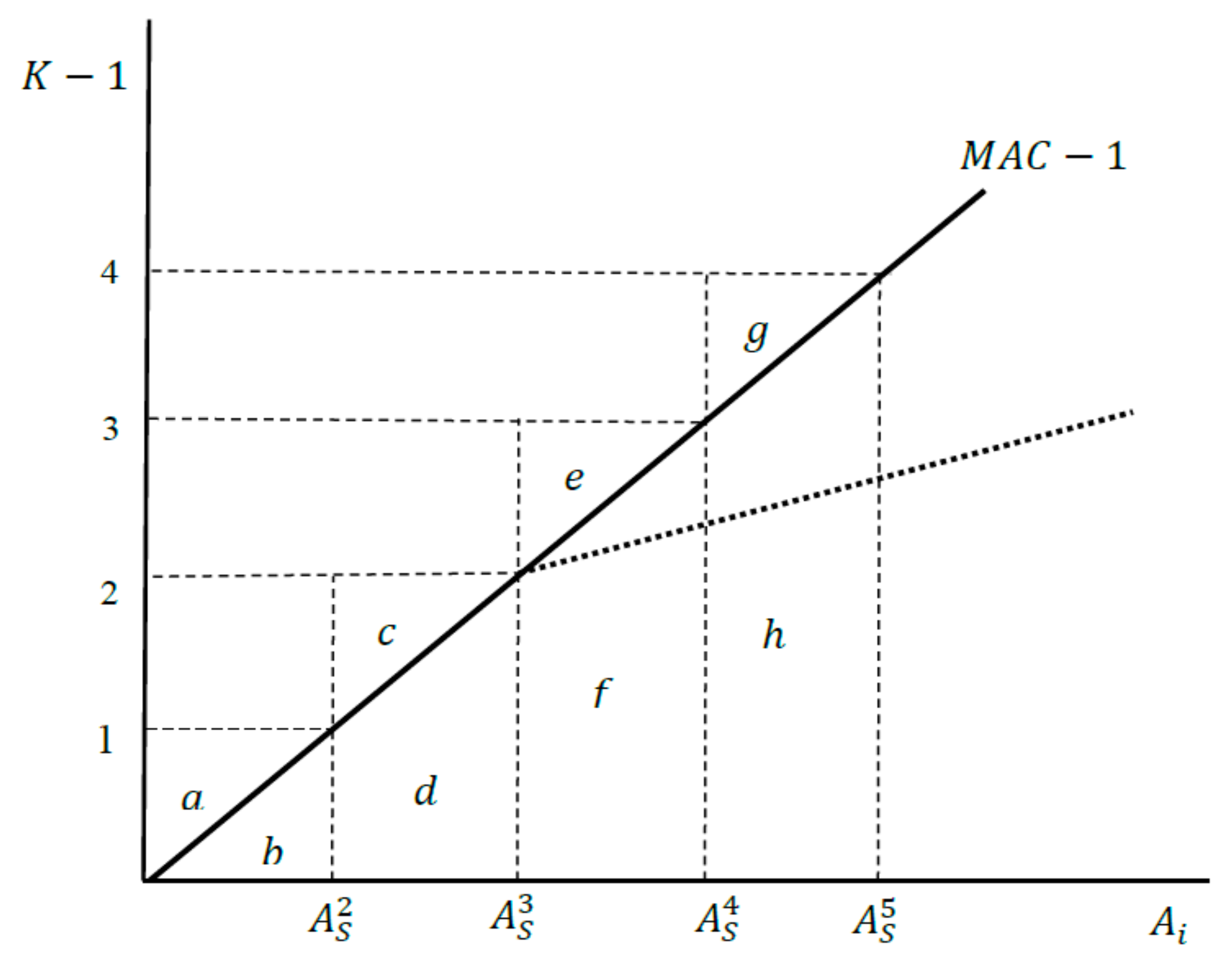
Why do large coalitions require huge increments in abatement to make additional entry attractive? The intuition behind the result can be explained by diagrams that simply depict the marginal abatement cost, , minus unity. They are based on those used by Karp/Simon ([4], p. 335). Assume initially that , i.e., the marginal abatement cost is linear, a signatory’s abatement is , and its marginal abatement cost is K. Figure 1 shows the curve, i.e., the marginal cost minus the marginal benefit of abatement accruing to the abating country itself. If a country chooses unilaterally instead of 0, it loses . If it does this as a member of a coalition , it benefits from the abatement of the other country and this benefit is such that the net gain is . If a third country enters a coalition with two members, its net loss from its own abatement effort is . The other countries increase their abatement from to Multiplying this by the number of countries increasing their abatement gives , depicted by in Figure 1. The net effect, , is zero. The fourth country considering entering this coalition has net cost and its gain from emission reduction by the coalition members is such that the overall benefit from joining is effect is . For the fifth country, this is even more negative: .
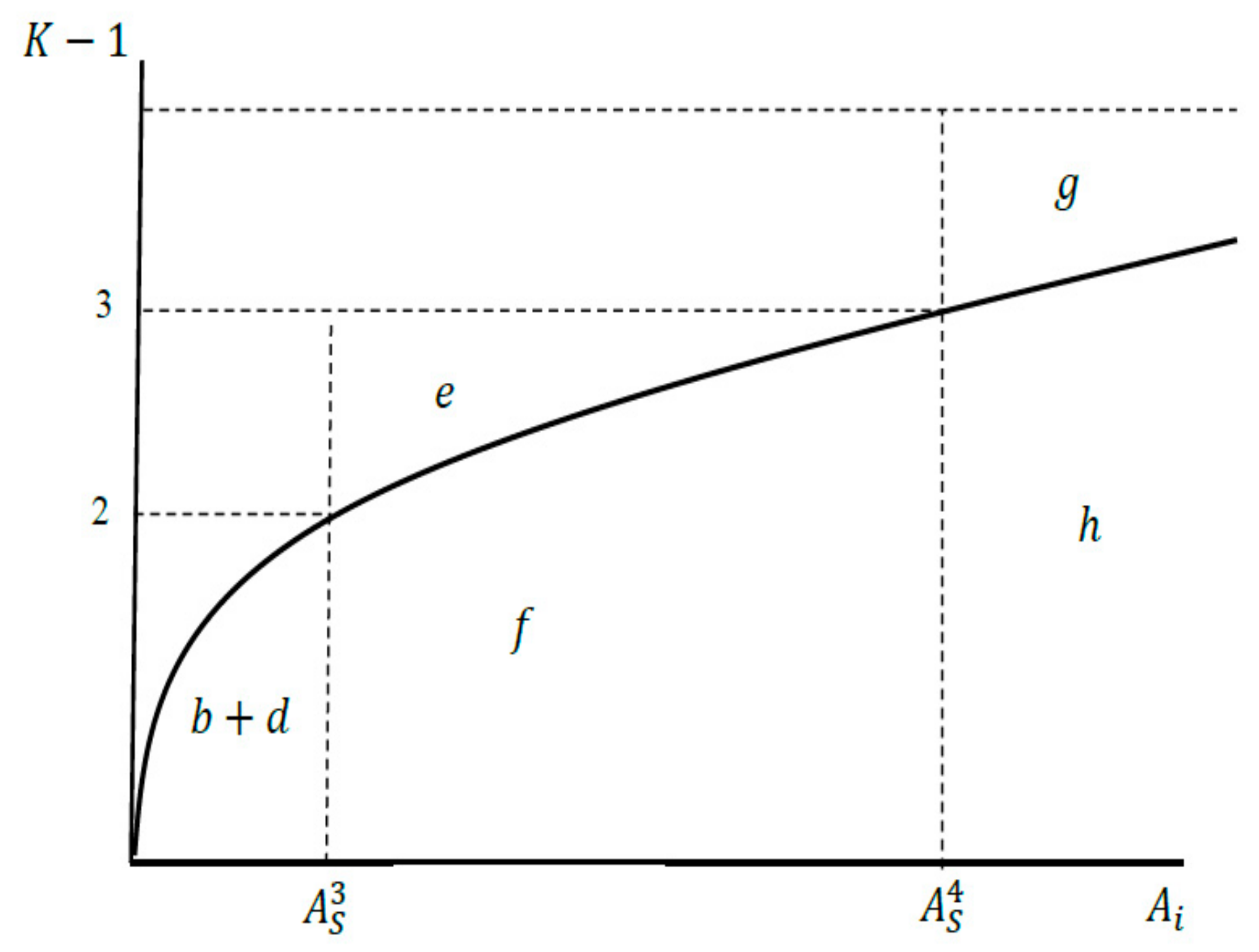
In order to make it profitable to an additional country to join an existing coalition , its members must do more additional abatement than in Figure 1. This implies that the curve needs to be concave as shown in Figure 2. The fourth country deciding whether or not to join a coalition of size has an additional net cost of whereas its benefit from additional abatement of the other countries is . Thus, the net benefit is , which in this case is positive. Stable coalitions larger than 4 require a marginal cost curve that is even more concave. Then the ratio of to will be even larger than that depicted in Figure 2. Since this incremental factor can be substantially larger than one and since such a factor is applied at every entry of a new signatory into the IEA, the abatement level must be very small for coalitions smaller than the grand coalition.
4. Modifications of the Model
It can be shown that increasing increments in abatement are necessary to obtain large stable coalitions with other specifications of the MAC function, too. In Karp/Simon [4], the concavity of the line was achieved by assuming kinks like the one depicted by the dotted line in Figure 1 to enlarge the triangles above . Such a kink must be drawn such that the modified triangle is as least as large as , which equals . As the size of triangle is , we have that . To make a fifth country join the coalition, the incremental factor must be even larger: and it can be shown that the incremental factor goes to as becomes large.2 Thus, basically the same considerations as in our model apply even if the MAC curve is not continuously differentiable, although the incremental factors are smaller than those in Table 1. The underlying reason for the smaller factors is that the kinks in the Karp/Simon model are constructed such that the additional country is indifferent between joining and not joining for all externally unstable coalitions, whereas our model implicitly assumes that all countries joining coalitions smaller than the stable coalition have strictly positive benefits.
The pessimistic result of the paper—i.e., that sizeable coalitions that are smaller than the grand coalition abate only a minuscule fraction of what is necessary to combat the global environmental problem—can be ‘repaired’ by assuming that the marginal abatement cost curve changes its shape once the stable coalition is reached. Let us look, for example, at a scenario where the MAC curve becomes linear once the stable coalition has been reached. One can show that in this case the emissions of a member of the grand coalition (which is internally unstable) and the emissions of a member of the stable coalition are related as follows 3
Using the values reported in Table 1, it is seen that for and a stable coalition of , this factor is 237.5 and that it increases to 350 for and . The underlying intuition is that the MAC curve is very flat when the stable coalition is reached such that additional abatement efforts must be very large. The Karp/Simon model will produce similar qualitative results, albeit less pronounced since the MAC curve is steeper than in this model.
The only way out of the dilemma that large coalitions achieve little is an S-shaped MAC curve becoming convex at the point where the stable coalition has been reached. Although an S-shaped curve is not a priori unrealistic,4 the condition that the change in curvature occurs exactly when the stable coalition is achieved is unlikely to be met. If this change prevails at a lower level of abatement, the stable coalition will be small. If it occurs at a higher level, the coalition will be large, but it will achieve little.
5. Summary and Conclusions
The paper has shown that stable coalitions with more than three members are possible in static games with orthogonal reaction functions and Nash behavior of the coalition if the marginal abatement cost curve is not linear like in the majority of the coalition-formation models, but concave. However, large coalitions smaller than the grand coalition achieve only a small fraction of what the grand coalition would achieve in terms of abatement. The underlying reason is that to create an incentive for a country to join a large coalition, the marginal abatement cost function must have properties ensuring that the existing members are willing to increase their abatement by a multiple after the accession of this country. In other words, the marginal abatement cost function must become very flat when abatement is increasing. Additional membership requires huge increases in abatement. This continues to hold for the unstable coalitions that are larger than the stable coalition, and particularly for the largest of these coalitions, the grand coalition. The only way out of the dilemma that large coalitions achieve little is a marginal cost curve that changes its curvature where the stable coalition is reached and becomes convex afterwards. Although such a change in curvature is not completely unrealistic, the requirement that this change occurs exactly at the abatement level chosen by members of the stable coalition definitely is. If the change occurs somewhere else, we are back at the starting point: either the stable coalition is very small or it is large, but achieves little.
An additional caveat is the assumption of linear benefits of abatement, implying orthogonal reaction functions and zero leakage. It is obvious that the results will be even less optimistic if benefits are concave and leakage matters.
Finally, although this paper is more conceptional than empirical by asking which conditions ought to be met to make large environmental agreements stable and at the same time effective, one might ask whether such conditions are met in reality. The widely cited global abatement-cost-curve by McKinsey and Company [13] claims that abatement costs are currently still negative for a range available options, then become almost linear (with some kinks) before turning convex for more ambitious abatement targets. Moreover, the Paris Agreement of 2015 has shown that countries are willing to take some action against climate change, but the efforts seem to be only partial. Game-theoretic models that explain why the members of the (almost) grand coalition comply only partially to their obligations are still lacking.
Funding
This research received no external funding.
Acknowledgments
I am indebted to Andreas Lange, two anonymous referees, and the editor for their comments and suggestions, which helped me to improve the paper. Any remaining errors and shortcomings are solely my own responsibility.
Conflicts of Interest
The author declares no conflict of interest.
References
- Barrett, S. Self-enforcing international environmental agreements. Oxf. Econ. Pap. 1994, 46, 878–894. [Google Scholar] [CrossRef]
- Carraro, C.; Siniscalco, D. Strategies for the international protection of the environment. J. Public Econ. 1993, 52, 309–328. [Google Scholar] [CrossRef]
- Finus, M. Game Theory and International Environmental Cooperation; Edward Elgar: Cheltenham, UK, 2001. [Google Scholar]
- Karp, L.; Simon, L. Participation games and international environmental agreements: A non-parametric model. J. Environ. Econ. Manag. 2013, 65, 326–344. [Google Scholar] [CrossRef]
- Diamantoudi, E.; Sartzetakis, E. Stable international environmental agreements: An analytical approach. J. Public Econ. Theory 2006, 8, 247–263. [Google Scholar] [CrossRef]
- Chander, P.; Tulkens, H. A core-theoretic solution to for the design of cooperative agreements on transfrontier pollution. Int. Tax Public Financ. 1995, 2, 279–293. [Google Scholar] [CrossRef]
- Chander, P.; Tulkens, H. The core of an economy with multilateral environmental externalities. Intern. J. Game Theory 1997, 26, 379–401. [Google Scholar] [CrossRef]
- Currarini, S.; Marini, M. A sequential approach to the characteristic function and the core in games with externalities. In Advances in Economic Design; Koray, S., Sertel, M.R., Eds.; Springer: Berlin, Germany, 2003; pp. 233–250. [Google Scholar]
- Marini, M. The sequential core of an economy with environmental externalities. Environ. Sci. 2013, 1, 79–82. [Google Scholar] [CrossRef] [Green Version]
- Carraro, C.; Siniscalco, D. R&D cooperation and the stability of international environmental agreements. In Environmental Negotiations: Strategic Policy Issues. Cheltenham; Carraro, C., Ed.; Edward Elgar: Cheltenham, UK, 1997. [Google Scholar]
- Helm, C.; Schmidt, R. Climate cooperation with technology investments and border carbon adjustment. Eur. Econ. Rev. 2015, 75, 112–130. [Google Scholar] [CrossRef] [Green Version]
- Katsoulacos, Y. R&D spillovers, cooperation, subsidies and international agreements. In International Environmental Negotiations: Strategic Policy Issues; Carraro, C., Ed.; Edward Elgar: Cheltenham, UK, 1997; pp. 97–109. [Google Scholar]
- Pathways to a Low-Carbon Economy: Version 2 of the Global Greenhouse Gas Abatement Cost Curve; McKinsey & Company: New York, NY, USA, 2009; Available online: https://www.mckinsey.com/business-functions/sustainability/our-insights/pathways-to-a-low-carbon-economy (accessed on 22 October 2019).
| 1 | Diamantoudi/Sartzetakis [5] find that the maximum coalition size in this case is reduced to 4 if the game is specified in terms of emissions instead of abatement and if a non-negativity constraint on emissions is imposed. |
| 2 | This can be shown by means of Figure 2. Although the marginal abatement cost function is strictly concave, the considerations carry over to piecewise linear functions. In the case of indifference whether to join or not to join, the areas and are equally large. A fifth country is willing to join if the benefit from additional abatement of the other countries, , is at least as large as its own net cost (abatement cost minus benefit from own abatement), . In the linear model of Karp/Simon [4], Thus the condition for the fifth country to enter is that . In general, the Kth country is willing to join if at least . This implies . For large , . Using this in the previous equation gives . |
| 3 | If the MAC curve becomes linear at , we have , where is the derivative of the marginal abatement cost. Using and rearranging terms yields the result. |
| 4 | S-shaped cost curves are common in economics, representing initially increasing and later decreasing returns to scale. An S-shaped marginal cost curve like the one proposed here implies slightly decreasing (almost constant) returns to scale if A is small and rapidly decreasing returns to scale if A is large, i.e., almost linear relationship between the abatement capital invested and the abated emissions until a threshold and extreme increases in investments required after the threshold to achieve further emission reductions. |
Figure 1.
Benefits from entering a coalition if .

Figure 2.
Benefits from entering a coalition if .


Table 1.
Critical coalition sizes, stable coalitions, and their properties for different values of .
Table 1.
Critical coalition sizes, stable coalitions, and their properties for different values of .
| 2 | 1 | 0.5 | 0.2 | 0.1 | 0.01 | |
| 1.8 | 2 | 2.37 | 3.32 | 4.69 | 22.17 | |
| 2 | 2 and 3 | 3 | 4 | 5 | 23 | |
| abatement increment, | – | 2 | 4 | 7.59 | 17.76 | 130.39 |
| share of GC abatement | 0.10 | 0.02 and 0.03 | 0.004 | 2.5*10–8 | 1.2*10–14 | 4.8*10–66 |
| share of GC global welfare | 0.03 | 0.0004 and 0.0009 | 0.0004 | 0.6*10–8 | 0.6*10–14 | 8.7*10–65 |
© 2019 by the author. Licensee MDPI, Basel, Switzerland. This article is an open access article distributed under the terms and conditions of the Creative Commons Attribution (CC BY) license (http://creativecommons.org/licenses/by/4.0/).
Share and Cite
MDPI and ACS Style
Rauscher, M. Stable International Environmental Agreements: Large Coalitions that Achieve Little. Games 2019, 10, 47. https://0-doi-org.brum.beds.ac.uk/10.3390/g10040047
AMA Style
Rauscher M. Stable International Environmental Agreements: Large Coalitions that Achieve Little. Games. 2019; 10(4):47. https://0-doi-org.brum.beds.ac.uk/10.3390/g10040047
Chicago/Turabian StyleRauscher, Michael. 2019. "Stable International Environmental Agreements: Large Coalitions that Achieve Little" Games 10, no. 4: 47. https://0-doi-org.brum.beds.ac.uk/10.3390/g10040047
Note that from the first issue of 2016, this journal uses article numbers instead of page numbers. See further details here.