The Role of Suggestions and Tips in Distorting a Third Party’s Decision

WZB Berlin Social Science Center, Reichpietschufer 50, D-10785 Berlin, Germany
Games 2020, 11(2), 23; https://0-doi-org.brum.beds.ac.uk/10.3390/g11020023
Submission received: 19 March 2020
/
Revised: 7 May 2020
/
Accepted: 11 May 2020
/
Published: 19 May 2020
(This article belongs to the Special Issue Experiments on Dishonesty in Strategic Interactions)
Abstract
:This paper experimentally investigates the impact of suggestive messages and tipping on a third party’s judgment. The experimental design uses a model with three players, wherein two players (A and B) create a joint project, and the third player (C) decides how to divide the project’s earnings between the first two players. In two treatments, player B has an opportunity to influence player C’s decision via a numeric message or an ex-post tip. The main finding of this paper is that giving player B the option to suggest a specific amount to the allocator does not increase his share. In contrast, when player C knows that player B can send him a tip, the share awarded to player B increases.
1. Introduction
When people talk about politicians favoring private interest, they generally assume that the main issue is that third parties bribe decision-makers. However, private parties may use alternative, more subtle, practices to achieve the goal of influencing decision-makers to obtain private benefits. Even if all mechanisms to exert influence on decision-makers are not necessarily corrupt by definition, the distortion of public officials’ decisions may harm society. Arguably, the most harmful aspect of bribery is neither the money spent on bribes nor the acceptance of these funds; it is the fact that decision-makers are influenced and that their decisions are distorted [1]. Therefore, if by using other channels of influence, subjects can achieve the same aim with almost no risk, then it is essential to study these alternative mechanisms.
Along this vein, how firms influence decision-makers is a central issue. The main reason is that it is unclear when a practice is illegal and when it is legal but unethical. For instance, in the US and Europe, it is legal for some private firms to lobby decision-makers. However, the crucial point is not the legality of this practice, but whether it biases the judgments of decision-makers. Existing research recognizes the critical role played by lobbying when influencing decision-makers. For instance, Campos and Giovannoni [2] provide empirical evidence showing that lobbying is more effective for gaining political influence than bribery. In the same direction, Moore et al. [3] argue that the failure of the US auditing system is not the result of bribery, but due to the lack of genuinely independent auditors. Additionally, Bennedsen et al. [4] show that large firms do not pay bribes, because they can use their political influence to circumvent laws and regulations instead.
In light of the preceding insights, this paper focuses on the efforts to influence decision-makers’ judgments and not on corruption through bribes, as many previous studies have done [5,6,7,8]. Specifically, this paper addresses the question of whether a suggestive message or a potential gift (tip) can affect the allocations made by a decision-maker in comparison to those made in an environment free of influence. To assess the causal effect of suggestions and tips on the decision-maker’s allocation, a laboratory experiment that varies these two components exogenously is used.
In the experiment, a game with three players is used, wherein two players create a joint pie, and the third player must decide how much of the pie to allocate to each of the first two players. The third player receives a fixed wage regardless of his decision, and the contribution of the first two players cannot be easily separated. The experimental design has three conditions: (1) The baseline treatment (FREE), (2) the advice treatment (AD), and (3) the tipping treatment (TIP). In FREE, there is no way to exert influence on the decision-maker. In AD, a channel for explicit influence is introduced, whereby one of the first two players can send a numerical message to the decision-maker suggesting a way to allocate the resources. In TIP, a channel for exerting influence in an implicit way is introduced, whereby it is common knowledge that one of the first two players will have the option of sending a tip to the decision-maker after learning the allocation.
The AD treatment stems from the fact that a simple way to try to take advantage of a connection with the decision-maker is by suggesting to him what to do. Indeed, in the political science literature, lobbying was initially modeled as a game of strategic information transmission [9]. This view regards lobbyists as better informed than decision-makers; consequently, the information transmitted by lobbyists enables politicians to make better decisions. However, Potters and van Winden [10] provide some theoretical arguments to state that the content of the message, as such, is not necessarily what transmits the information. They argue, instead, that it is merely the fact that a message is being received that is relevant.
It is possible to relate this latter point to the work of Schultze et al. [11], who show that receiving advice creates an anchoring effect that influences the decision-maker. This mechanism has been studied by Rankin [12] and Andersson et al. [13], who find a relationship between the amount claimed and the amount offered in an ultimatum game with communication. Ben-Ner et al. [14] also find that, in a trust game, communication increases trust and trustworthiness, even if the type of message is numerical. Hence, with the AD treatment, this paper contributes to the discussion by assessing whether sending a numerical message, that is, merely a suggestion that does not convey any critical information beyond the desire of the sender, influences the decision-maker.
The TIP treatment assesses whether a potential tip biases the decision-maker. In this particular case, expected reciprocity may play a role that ultimately generates a negative externality for a third party. Notice that the bias relies on the effect of reciprocity, because if a player is purely selfish, it is not rational for him to give money to strangers when there is no legal requirement to do so or any tangible benefit to gain. In this direction, there is a vast amount of experimental literature that provides evidence of reciprocity as a mechanism for establishing gift exchange relations [15,16]. Although reciprocity may be beneficial in some social relationships, Abbink [17], Weisel and Shalvi [18], and Malmendier and Schmidt [19] provide evidence of a dark side of reciprocity. In particular, these scholars show that reciprocity serves as a contract device between two parties who are involved in corruption. The results found by Malmendier and Schmidt [19] are closely related to this paper because they show that small gifts strongly influence the receiver (i.e., the decision-maker). However, the main difference between the bribery literature and this paper is the moment when the gift is received. For instance, in the works of Abbink et al. [7], Abbink [17], and Malmendier and Schmidt [19], the gift (i.e., the bribe) is given before the decision-maker decides, whereas in this paper, gifts are given after the decision is made. Thus, in this paper, the impact of reciprocity is not studied in the standard way, that is, a third party gives money to distort the decision-maker’s judgment. In contrast, whether the decision-maker favors a potential tipper at the expense of others because he wants to be worthy of a tip is studied instead.
Although ex-post gifts may seem unrealistic and irrelevant, there is some evidence that provides insights into their potential role in exerting influence. Austen-Smith and Wright [20] show that lobbyists address politicians who have similar interests to them, but also politicians who are reluctant to support them. In the first case, the gifts may come ex-post because politicians already know that some firms will reward them if they pass a bill. In line with this argument, You [21] found that roughly 50% of the lobbying activity in the US from 1998 to 2012 happened after a bill was passed.
The main result of the AD treatment shows that suggestions sent by a stranger do not have a significant impact on the decision-maker’s allocation. This result contributes to the discussion on lobbying by providing evidence that supports the view that receiving a message may not be influential per se. On the other hand, in the TIP treatment, potential tips bias the decision-maker’s judgment in favor of the potential tipper. This result is in line with the strand of literature suggesting that reciprocity is crucial for establishing unethical relations. However, in a tipping scenario, the reciprocal relationship begins with the decision-maker instead of the private party. Therefore, the results herein suggest that expected reciprocal responses may have a similar effect on decision-making than actual reciprocity. Specifically, it is found that expecting an ex-post gift generates similar results to bribery but with a lower risk.
The remainder of the paper is organized as follows. Section 2 presents the theoretical framework and predictions: the complexity of the decision-maker’s choice is explained, and some solutions to the allocation task are provided. Section 3 outlines the experimental design, procedure, and hypotheses. Section 4 presents the main results of the experiment. Finally, in Section 5, the implications of the results are discussed, and some concluding remarks are offered.
2. Theoretical Framework
2.1. Influence Game and Equilibrium Characterization
The model is based on a four-stage game involving three players. In particular, there are two players involved in the creation of a surplus. Both players contribute inputs that are not easily comparable because they use different units of measurement. After that, a third party decides how to divide the surplus created. It is important to mention that this game does not directly mimic a real-life situation, nor does it pretend to do so. Nevertheless, it captures two specific situations. First, the production phase of the game represents situations in which groups of people contribute to a joint product. However, each member’s input is in different units of measurement, and each subject is indispensable for having a positive outcome. In other words, it represents situations in which equal divisions are the more intuitive way to distribute the benefits of an outcome, because it is difficult or even impossible to evaluate people’s contributions.
Second, the allocation phase represents situations in which a decision-maker has to solve a dispute between two parties. This second part is the main focus of the paper, because it may have implications for policy making. For instance, it relates to judges who take decisions that involve agents with competing interests, it also applies to politicians who decide on how to allocate a new construction project between contractors, or a manager who has to decide on how to divide a bonus between members of a group, and so forth. In general, the author of this paper is interested in situations in which ensuring the independence of the person who solves an allocation problem is a crucial point.
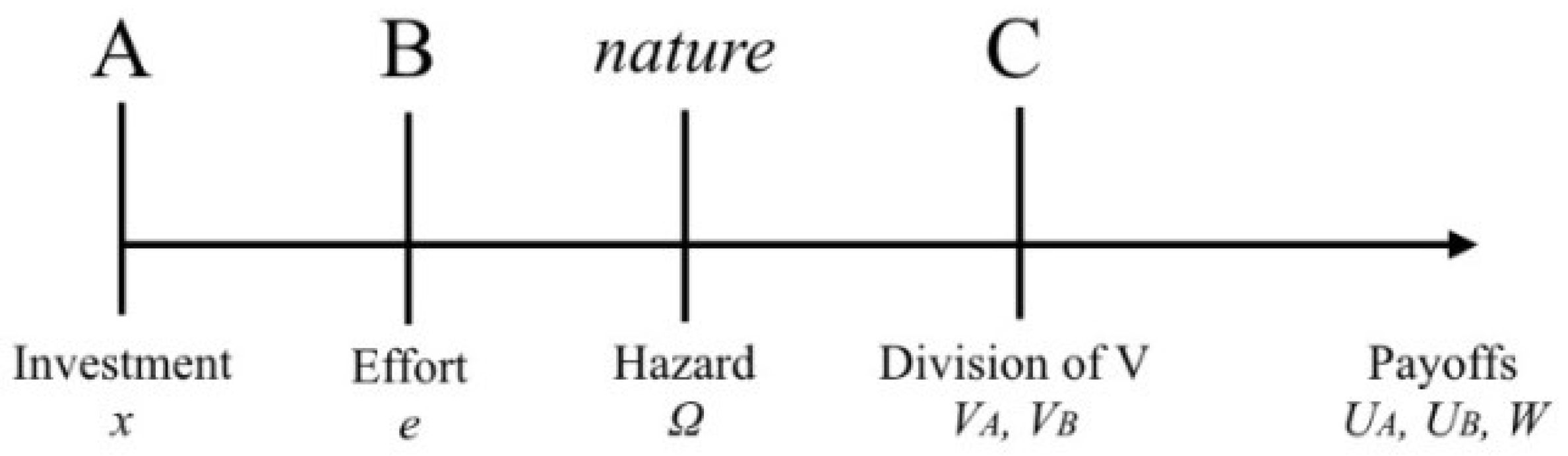
In stage 1, player A,1 endowed with , chooses the part of her endowment, x, that will be invested in a joint project, where . The remaining money is retained in her private account. In stage 2, player B observes x and decides on a level of effort, e. Player B pays a cost for the chosen level of effort. The function determines the specific cost for each e, where c (e) increases exponentially with the non-negative level of effort.2 The sequence of decisions in the influence game is presented in Figure 1.
In stage 3, once players A and B have made their choices, nature defines the general economic conditions of the game , with . Nature draws randomly from a uniform distribution. Thus, the expected value of is zero, but the probability that the value of is precisely zero in a one-shot game is considerably low. Player B’s resulting output (or his performance) depends on his chosen effort (e) and nature’s economic conditions (). Specifically, player B’s output is given by , where . As in the works of Bull et al. [23], Schotter et al. [22], and Fehr and Schmidt [24], the function f(.) is concave, and is a random shock. Hence, player B contributes to the project an effort that is not directly observable, but that generates an observable output, y, which is a signal of his effort.
The value of the resulting project, v, is the product of player A’s investment and player B’s output, i.e., v = xy. Given this outcome, in stage 4, player C decides how to divide v between players A and B. Importantly, player C observes x, y, and v, but does not observe e or . In this paper, a non-deterministic output, y, is used to make it more difficult for player C to justify favoritism for B, and thus to make a 50–50 distribution salient. It is important to highlight that player C has a fixed wage, ; therefore, his material gains are independent of the allocation. In particular, the allocation for A and B are such that . The payoffs for players A, B, and C are given by the function below:
Proposition 1 presents the subgame perfect Nash equilibrium of the game:
Proposition 1.
In the influence game, the best response for player A is if her belief about the part of the pie allocated to her will be at least as good as keeping all the endowment, or otherwise. The best response of player B is , where is the belief about the fraction of the pie that will be allocated to him.
Proof.
The proof is included in Appendix A. □
Here, it is assumed that γ is the same for player A and player B, and that the players are risk neutral. These assumptions simplify the analysis and relaxing it will not change the conclusions of the theoretical analysis. Proposition 1 implies that the game has multiple equilibria, including some in which the value of the pie is zero. The intuition behind Proposition 1 is as follows: In the last stage, player C divides the value of the project between players A and B. Player C has no material incentives because of the flat wage; thus, if he is selfish and rational, he will be indifferent to any form of sharing. Player B has a belief about how the third party will divide the pie, so he will exert the optimal effort in relation to his belief. As a consequence, player A will invest her entire endowment in the joint project to maximize the value of the final pie, and therefore her profit, as long as the expected return, , is higher than her endowment.
2.2. The Third-Party Decision
As mentioned before, in the baseline, the decision-maker has no material incentives for any particular division of the pie. Hence, he could choose randomly how to allocate the resources between players A and B. However, assuming a random allocation implies that the decision-maker only cares about material gains. Instead, in this paper, it is assumed that the decision-maker wants to appear as a fair person. This assumption is in line with the literature on social preferences, which have been studied using ultimatum games and dictator games [25]. In other words, it is assumed that the utility of player C is a combination of his income and a desire for fairness. Following Cappelen et al. [26], an assumption is made that player C will use the equal division of the income as the fairness norm. The utility function of the decision-maker that incorporates this norm can be represented by:
The first-order condition of the utility function (2) will lead to a 50–50 distribution. This solution is also consistent with the literature on inequality aversion [27]. It is worth noting that this equal division of the total revenue does not incorporate the cost of effort. There are two particular reasons for that. First, even if the expected value of Ω is zero, in each round, player C does not know the realization of Ω. Thus, the real value of player B’s effort is private information; then, it is impossible to discount the real cost of effort for a particular realization. Second, the decision-maker is not necessarily interested in being fair, but in being perceived as fair. Hence, the most salient way to look like a fair person is making a 50–50 division of the total pie.
3. Experimental Design
3.1. Treatments
Two treatments were used to assess the causal effect of suggestions and tips on how player C distributes the value of the project between players A and B. In the treatments AD and TIP, player B is the treated agent, i.e., he is the player that can exert some influence on player C. It was decided to treat player B because the third party cannot observe his real effort. Consequently, it is easy to isolate the influence mechanism from the contribution to the project that is under player B’s control. It is believed that even if the results may have differed if player A was the one treated, the central message of the paper is not undermined by treating only player B.
3.1.1. Baseline Treatment (FREE)
The FREE treatment serves as the baseline for this study. In the influence game, there are groups of three participants. Participants play 10 rounds. A strangers matching protocol is used with fixed roles. In every round, player A is endowed with points, from which she can make her investment choice . Player B can exert effort , at the cost of . The value of λ is 1.5, and the exogenous shock is . To make the instructions easier for the participants to understand, player B is asked to choose an effort that already incorporates a , i.e., .3 Once the value of the project is known, player A and player B are asked about their beliefs regarding the share of the pie that they expect to receive.4 At the same time, player C learns player A’s investment (x), player B’s output (y), and the final value of the project (v). Finally, player C allocates v, and both players A and B are informed of their share in the current period. Based on proposition 1, the hypothesis about the participants’ behavior in FREE is:
Hypothesis 1.
In FREE, player A will invest her entire endowment, player B will exert the optimal effort, and player C will divide v equitably between players A and B.
3.1.2. Advice Treatment (AD)
In the AD treatment, a one-way communication channel is introduced to enable player B to send a message to player C. The message can be sent once player B knows the value of the project, v, and before player C decides how to distribute it. The message has a preset text, and the sender only needs to insert a numerical value that he is suggesting to player C as a share for him. This type of message was chosen to keep control of the suggested amount and to assess whether it correlates with the sharing decisions. If this cold communication channel can bias player C’s decision, then more rich ways, such as free-form chat, will do so as well.
The existence of the communication channel is common knowledge among all participants. However, player A is not informed of whether or not player B has sent a message. Thus, complete anonymity concerning the decision is ensured. The motivation behind the AD treatment is based on empirical evidence suggesting that cheap talk can alter the equilibrium play. For instance, Rankin [12] and Andersson et al. [13] observe that, in ultimatum games, cheap talk decreases the sender’s payoff. Ben-Ner et al. [14] find that reciprocal relations in a trust game are increased with the introduction of a communication channel, even if it is just numerical communication. In this experiment, it is expected that the suggestion creates an anchor, and as a consequence, the share for player B will be higher than in FREE. Given proposition 1, the belief about the share that player B will receive (γ) is higher than in FREE. Hence, player B’s optimal effort is higher. In line with this, the behavioral prediction for the AD treatment is presented in Hypothesis 2:
Hypothesis 2.
In AD, player B will exert an effort higher than in the baseline and will make use of the communication channel, and player C will allocate a larger share of v to player B than in FREE.
3.1.3. Tipping Treatment (TIP)
In the TIP treatment, the effect of a potential ex-post bribe on the decision-maker’s allocation is studied. Once the value of the project is known and player C has divided v between players A and B, player B can send a tip to player C. The potential tip is common knowledge, and therefore, player C is aware of this possibility when allocating. In other words, the reciprocal response of player C to a tip is not assessed, but rather the distortion in the share for player B due to player C looking for a reciprocal response is analyzed. Note that a selfish player B should never send a tip to player C once the allocation of v has taken place. Therefore, in a selfish and rational world, player C anticipates this and behaves as in FREE. However, some behavioral insights lead one to believe that this behavior may be different when people are making decisions in real life. For instance, Azar [28] shows that the presence of potential tips improves the quality of service, which in the influence game would mean that player C may favor player B in TIP. In the works of Abbink et al. [6,7], Abbink [29], and Weisel and Shalvi [18], the authors show that reciprocity is essential for corruption to occur. This result may apply not only to bribery, but to all types of corruption in general. Therefore, here, it is argued that when player C knows that player B can send him a tip, player C may decide to allocate a bigger part of the pie to player B in order to receive a reciprocal response. Thus, it is hypothesized that the seeking of tips influences player C’s behavior in favor of player B, even without them having previously reached an agreement. This is based on the assumption that the potential impact of tipping is supported by reciprocity [30], social norms [31], and fairness [28], instead of self-interest. The prediction for the TIP treatment is presented in Hypothesis 3:
Hypothesis 3.
In TIP, player B will exert a higher level of effort, and player C will allocate a larger share of v to player B than in FREE.
3.2. Procedures
The experiment was conducted in the GATE laboratory at the University Lumière Lyon 2 and the University Jean Moulin Lyon 3. A total of 252 people participated in the study (102 in FREE, 87 in AD, and 63 in TIP). Each participant participated in one treatment only. Participants were all undergraduate students from the universities who interacted via computers using z-Tree [32]. Standard experimental procedures were used, including neutrally worded instructions. The instructions are presented in Appendix B.
Participants played the influence game for 10 periods following a strangers matching protocol with fixed roles. That is, the composition of the groups changed in every period. However, the roles of player A, player B, and player C were randomly assigned at the beginning of the experiment and remained fixed throughout the 10 periods of play. After the 10 periods of the influence game, participants played two modified dictator games using choice menus. These two choice menus were used to create a control for inequality aversion. In particular, they allowed to estimate the parameters α and β of Fehr and Schmidt’s model5 [27]. On the one hand, the parameter α measures the utility loss from disadvantageous inequality (i.e., envy parameter), and parameter β measures the loss from advantageous inequality (i.e., guilt parameter). The explanation of how these measures were collected and constructed is presented in Appendix C. At the very end of each experimental session, participants answered a questionnaire with demographic questions. Participants were paid the amount they earned in one randomly chosen period of the influence game, the earnings in the dictator games, and a show-up fee. Participants earned around 12.9 euros on average.
4. Results
First is a summary of descriptive statistics for the choices in the influence game by treatment (see Table 1). For ease of illustration, the main variables were normalized between 0 and 1. The meaning of each variable used is as follows: Player A’s Investment choice (x) was normalized by dividing it by her total endowment (). Player B’s chosen Effort (e) was divided by the maximum level of effort (). Similarly, the value of the project was normalized by dividing it by the largest value that could be produced (). Belief A, Belief B, Advice from B, and Share for B were divided by the value of the project that was actually produced, while Tip from B was divided by the share B receives (Share for B).6
4.1. The Free of Influence Game
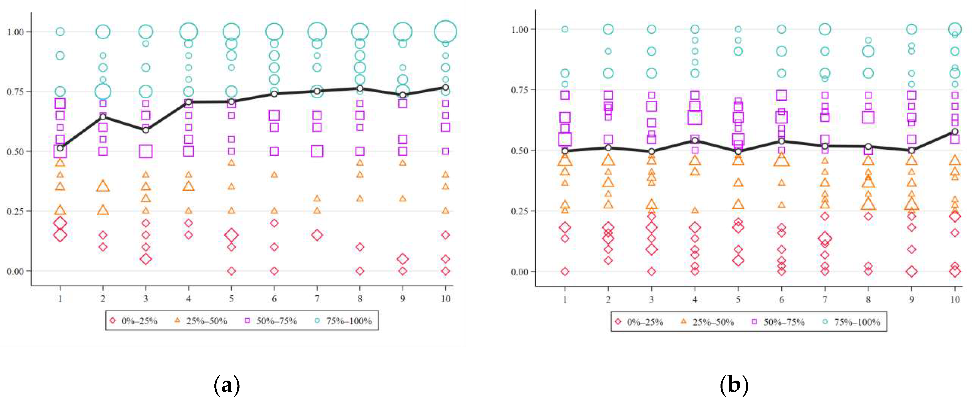
In the FREE treatment, any external factor that might influence player C’s distribution decision was controlled for. Subjects in the role of player A invested, on average, 69% of their endowment (see Table 1). This investment suggests that participants in the role of player A did not sufficiently attempt to achieve the highest project value. However, using Pearson’s correlation test,7 it can be observed that player A’s investment increases over time (r = 0.237, n = 340). Figure 2a shows that the frequency of high levels of investment, i.e., above 75%, increases over time, while the frequency of low levels of investment, i.e., below 25%, decreases (see circles and diamonds respectively, in Figure 2a). Despite this increase in high levels of investment, the average investment in the last round is significantly lower than the one predicted in equilibrium.
The evolution of the level of effort chosen over time, unlike that of the investment, is very steady (see Figure 2b). Using Pearson’s correlation test between the effort chosen and the period, it can be observed that the linear relationship between effort and time is positive but very weak (r = 0.045, n = 340). Finally, it is determined whether player B’s chosen effort best responds to player A’s investment. The results show that the effort exerted is significantly higher than the optimal level for the observed investment. The uncertainty around the effort choices could explain this result. Player B may be afraid that the negative shock may hit, and Player C may punish him for not trying hard enough.
Once the value of the project is known, both player A and player B report their beliefs regarding the share they expect to receive from player C. Player A’s expectations are significantly higher than those of player B, i.e., 0.55 > 0.51 (t = 3.5, p < 0.001). Nonetheless, player C’s mean choice is a 50–50 split, resulting in no significant difference in the allocation between players A and B (t = −1.10, p = 0.27).
Given that a repeated game with a strangers matching protocol was used, there may exist potential spillovers across subjects in the same session. To address this issue and any potential interdependence of observations, some random-effects General Least Squares (GLS) models were used with standard errors adjusted for clusters by sessions. Panel data models were used because the roles of participants were fixed, resulting in a panel with 10 periods for each subject. In the regressions, experience in the game (Period), player A’s investment (Investment), player B’s observable output, y (Player B output), the value of the project, the inequality aversion (Alpha and Beta F&S), and some demographics were controlled for.
Table 2 presents the results of a regression analyzing player C’s decision in the baseline treatment. The dependent variable in regression (1) is the percentage of the project allocated to player B. The coefficients of Investment and Player B output in regression (1) show that player C takes the investment of player A and the effort of player B into account when allocating the pie. Moreover, the coefficient of the variable Value of the project shows that there is a weak effect, whereby the greater the value of the project, the higher the allocation to player B. Regression (2) shows that these results are robust when controlling for the learning effect, as well as the end effect (after dropping periods 1 and 10). The latter effect is based on Crawford’s work [33], which shows that behavior in the laboratory often takes time to stabilize. Thus, dropping period 1 helps to account for some learning effects. In addition, Roth, Murnighan, and Schoumaker [34] show that there is a deadline effect in experiments that causes a change in behavior in the last period. Thus, the observations made in period 10 were dropped.
Result 1.
Without external influence, player C (the decision-maker) makes a 50–50 split of the value of the project between player A and player B.
4.2. The Effect of Messages
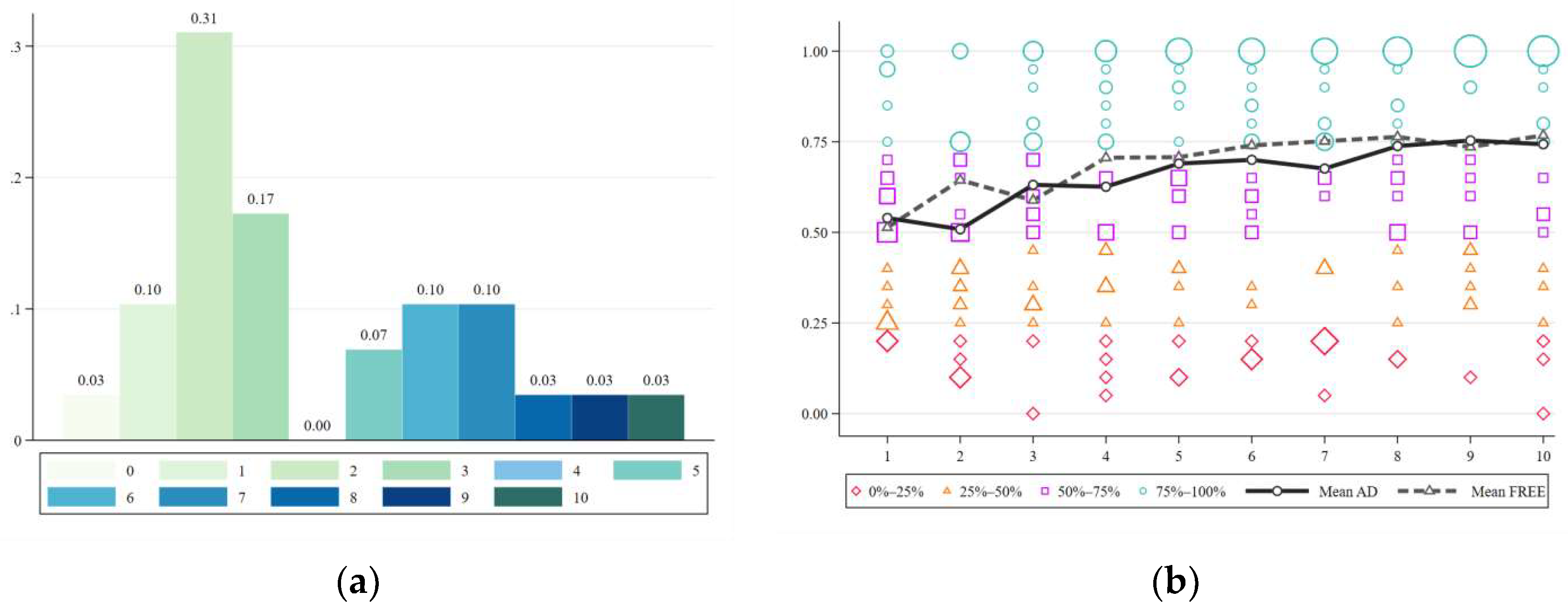
In the AD treatment, the effect of player B sending a message to player C, where he suggests a particular share of the project, was studied. Hypothesis 2 predicts that subjects in the role of player B will make use of the communication channel, influencing player C’s allocation in favor of player B compared with that in the FREE treatment. The data show that when considering all 290 interactions (29 groups over 10 periods), 178 (69%) did not include any message. To study in more depth the use of the communication channel, a score variable that counts how many times a player B sends a suggestion to player C over the 10 periods was created. Therefore, this score takes values between 0 and 10. Figure 3a presents a histogram for this advice score. It can be observed that 62% of the participants sent, at most, three messages (see Figure 3a). Thus, the evidence provides no support for the prediction of Hypothesis 2 regarding the use of messages. The little use of the communication channel can be explained by the fact that player C does not respond to suggestions. In period 1, about 60% of the participants sent messages, but after that, the percentage declined significantly.
Given that player A does not receive any information regarding messages, their choices were considered to be independent of the use of the communication channel. The average investment in the AD treatment is not different from that in the FREE treatment, as confirmed by a regression using investment as the dependent variable (see Appendix D). This result suggests that player A’s investments are not affected by the possibility player B has of sending a message to player C, which is in line with proposition 1. The trend over time increases, as shown in Figure 3b.
Subjects in the role of player B vary significantly in terms of their effort exerted, depending on whether they sent a message (M) or otherwise (NM). The average effort exerted is higher in the M group than in the NM group (p < 0.001), which provides some evidence about the sensitivity of effort to changes in γ. Moreover, player B’s effort in the NM group is significantly lower than in the FREE (p < 0.05), as presented in regression (3) of Appendix D, Table A4.
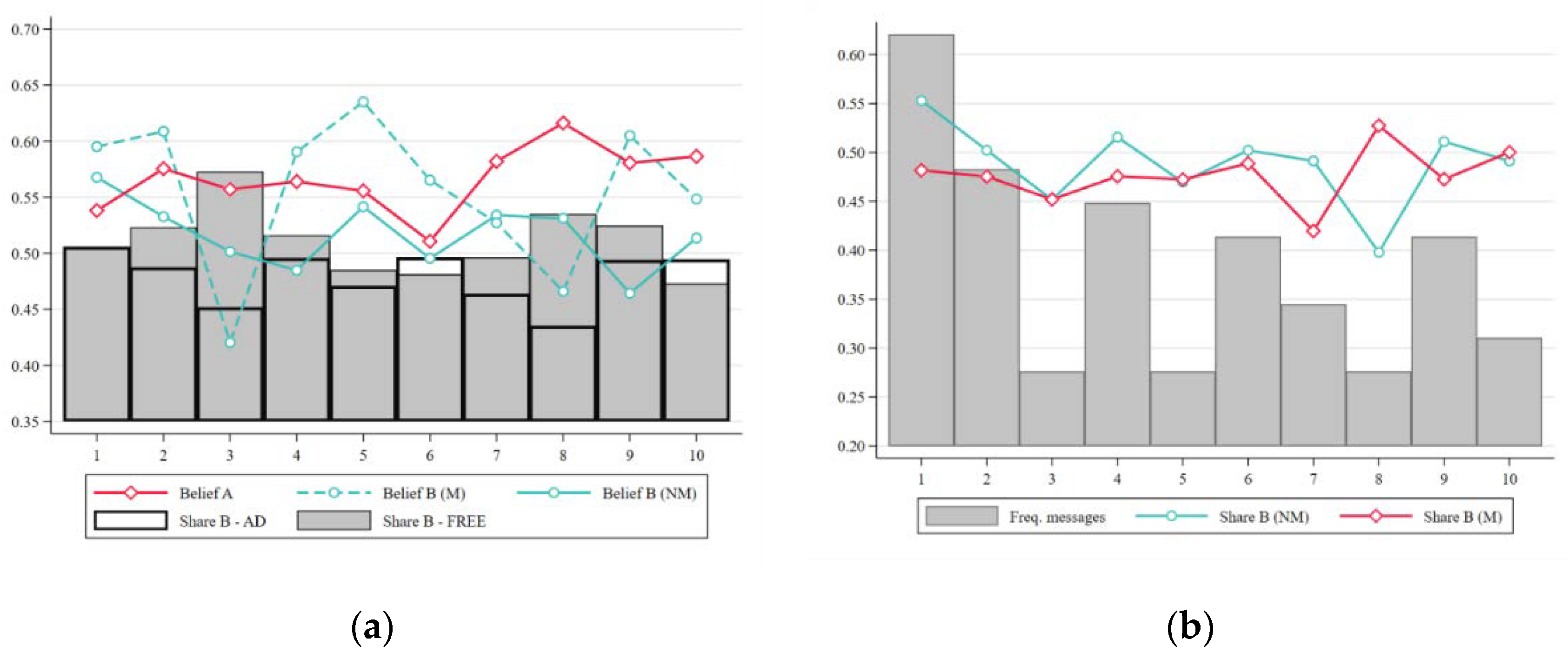
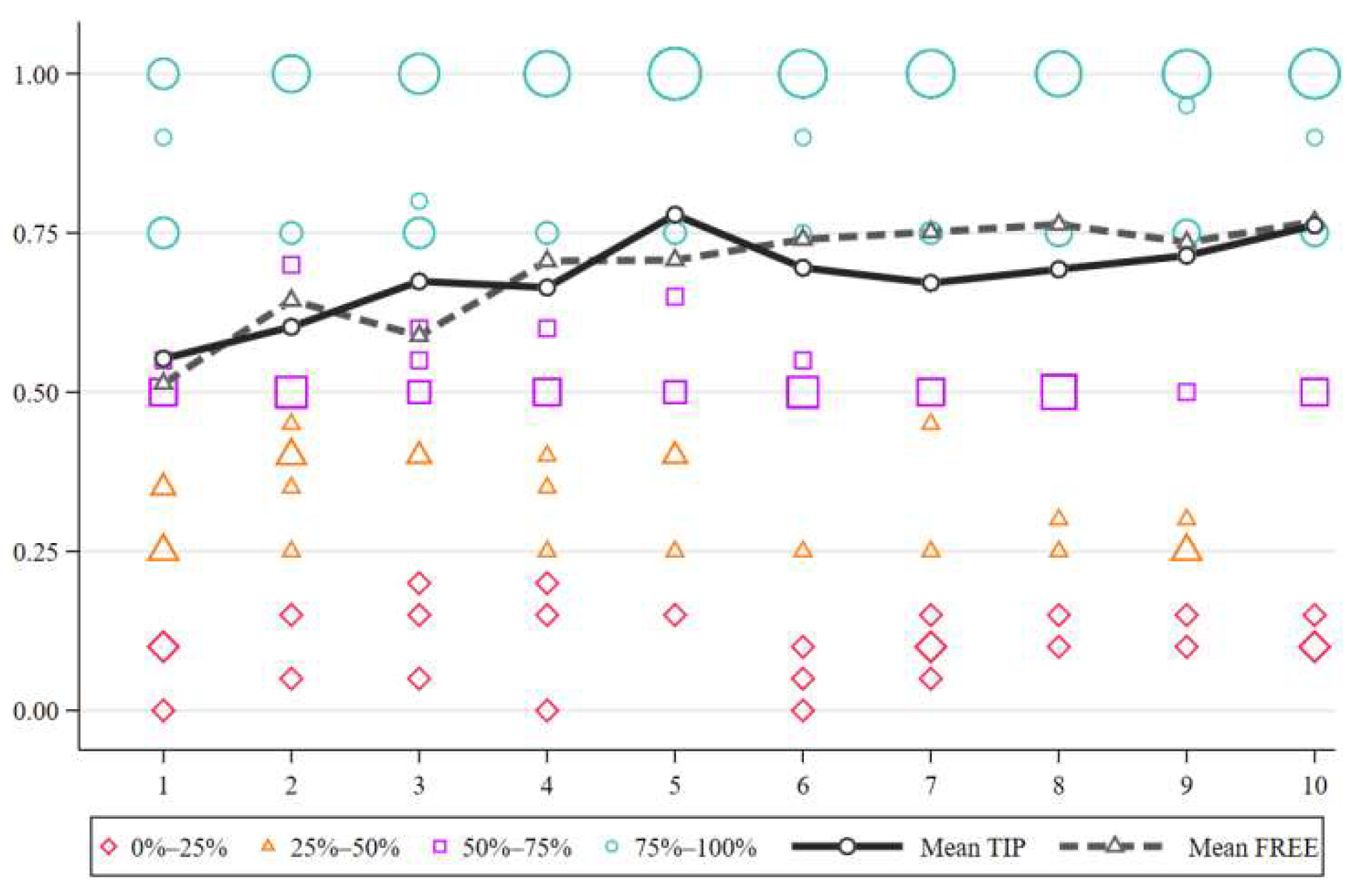
In the 38.6% of the interactions in which a message was sent, the average advice suggested an allocation of 62% of the value of the project to player B, which is positively and strongly correlated with player B’s beliefs in the M group (r = 0.59, n = 111). As illustrated in Figure 4a, on average, players who sent a message reported higher beliefs than those who did not send a message (z = 2.699, p = 0.0069). Conversely, player A’s beliefs are the same in FREE and in AD (p = 0.331), reinforcing the point that messages have no impact on player A’s behavior or expectations.
Table 3 presents some regressions similar to the ones presented in Table 1. The difference is that in Table 2, dummy variables are included to assess the effect of the treatment variations in the decision-maker’s decision. In models (1) and (2), the variable AD is not significant, which implies that player C’s allocation is not significantly different in AD than in FREE, suggesting a 50–50 split strategy8. Also, models (3) and (4) show that sending a message neither increases nor decreases player B’s share, as can be seen in the variable Message sent.
Result 2:
The use of suggestions does not affectplayer C’s or player A’s choices compared with that in FREE.
4.3. The Effect of Tips
In the TIP treatment, the effect of the possibility that player B sends a tip to player C once the allocation has been decided is studied. Hypothesis 3 predicts that player C will favor player B in the apportionment of the project value compared with the apportionment in FREE, and in return, player B will send a tip to player C. The investment is assumed to be the same as that in FREE, and the level of effort is predicted to be higher in TIP compared with that in FREE. The data show that out of the 210 interactions, i.e., 21 groups over 10 periods, a positive tip was sent in less than half of the interactions. Less than 5% of the participants either always sent a tip or never sent a tip, while the others were distributed across the range, sending from one to nine tips, with the most popular choices being two (19%), five (24%), and seven tips (14%).
In the TIP, the average investment is seemingly similar to that in FREE, as presented in Table 1. Indeed, comparing Figure 2a and Figure 5, one can see that the levels of investment are similar. However, after the period and demographics are controlled for, the investment in TIP is slightly higher than in FREE (p = 0.033), as is presented in regression (1) in Table A4 of Appendix D. Regression (2) in Table A4 of Appendix D shows that the level of effort is not significantly different between TIP and FREE.
In TIP, player A’s beliefs are significantly lower than in FREE (p < 0.001), as can be observed in regression (3) in Table A4 of Appendix D. This result implies that player A anticipates that the presence of a potential tip harms her allocation. Conversely, player B’s beliefs are significantly higher than in FREE (p < 0.01), as presented in regression (4) in Table A4 of Appendix D.
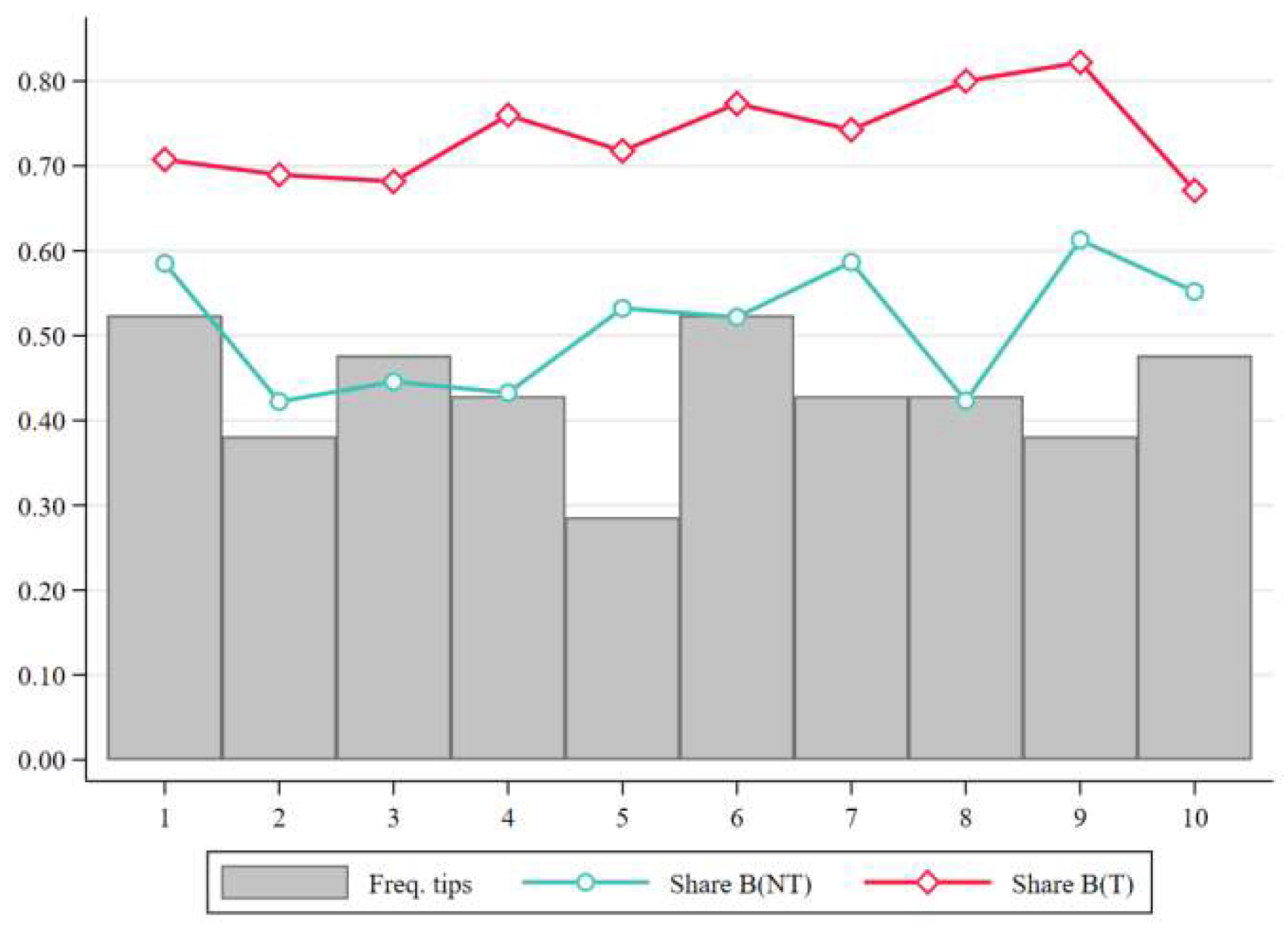
As mentioned in the experimental design section, arguably, the influence of a tip is that it creates in player C a willingness to favor player B in order to receive said tip. As can be seen in the coefficient of TIP in models (1) and (2) of Table 3, in TIP, player B receives 0.137 percentage points more than player A after controlling for several variables, including player B’s signal of effort. This result suggests that the possibility of receiving tips corrupts the judgment of player C in favor of the potential tipper. That is, the bias toward player B is the result of the assumption that player B will return some of the money allocated, thereby harming player A. To see this point, the players divided into those who sent a tip (T) and those who did not send a tip (NT). Figure 6 shows that player C’s distribution choices significantly favor player B over player A in the T group, while the allocation to B is around 0.5 in the NT group. In model (5) of Table A4 of Appendix D, a panel Probit model was used, in which the dependent variable is whether player B decides to send a tip or not. In this regression, the coefficient of Share to B is significant (p < 0.05), which suggests that the allocation of a higher share to player B triggers a tip from player B to player C.
Result 3.
The allocation to player B is higher in TIP compared with that in FREE. Those B players who receive a higher share of the project value are more likely to send a tip.
5. Discussion and Conclusions
The primary goal of the experiment was to determine whether the two mechanisms of influence distorted the independence of the decision-maker. Hence, all of the results should be interpreted in comparison with that in FREE. The AD and the TIP treatments were not compared directly, because these two treatments have more than one variation between them. The results provided two main findings. First, no evidence was found to show that the possibility of sending suggestions changed the share of the pie allocated to the player who sends the message. Second, the results provided strong evidence of the harmful role of reciprocity, given that the ability to provide tips increased the share received by player B by approximately 0.13 percentage points. This result is in agreement with the works of Azar [28] and Malmendier and Schmidt [19], who showed that reciprocity is vital for establishing gift-giving relationships in an ex-post or ex-ante scenario. Therefore, in this paper, a feeling of fairness is intuitively incorporated in player C’s expectations, causing his independence to be affected. In particular, the results suggest that seeking a reciprocal response may be as pervasive as being the object of bribery. A direct comparison between tipping and bribery is beyond the scope of this paper; therefore, further work needs to be done in this direction.
In addition, the evidence from this study suggests that the opportunity to gain access to the decision-maker does not necessarily imply that this connection can influence the decision-maker’s decision. Messages may prove useful if there is a more reliable link between the sender of the message and the receiver, but in the current experiment, the sender was a stranger in a one-shot interaction. A stranger matching protocol was used in this study to avoid any social ties in order to assess whether a message by itself can bias a third party by establishing an anchor. Some robustness checks of the results in AD and in TIP were conducted by analyzing periods 1 to 5 and 6 to 10 separately to capture some potential spillovers from one period to another. The regressions are presented in Appendix D. It can be found that the results presented in the previous section remain the same or become even more robust in the last five periods. However, it is worth undertaking further research incorporating social ties, by including repeated interactions or existing social ties, to assess whether a communication mechanism influences a decision-maker who has a social tie with the sender of the message.
Conversely, the results concerning tipping illustrate that creating an expectation of future reward is effective in influencing a third party. Nevertheless, the way in which to create this expectation of a tip was not studied, but rather what happens when this option is already created. It was found that the potential ex-post monetary gift has a similar effect to the one documented by Malmendier and Schmidt [19] for bribes. Thus, this result suggests that one should not underestimate these types of channels of influence. In the current game, decision-makers may argue that deviations from a 50–50 allocation are not necessarily unethical, and they can often justify their unequal allocations. This moral wiggle room is possible because they can always replace the image norm of an equal division of revenue with one of an equal profit division. However, the baseline treatment provides a proper contrafactual, which enables to see how decision-makers divide the pie without any influence. Hence, the implicit channel of potential in which there is a hope of receiving a tip exerts a bias on decision-makers’ judgments, whether consciously or unconsciously.
Funding
This research was supported by a grant from the Universidad Católica de Colombia, the WZB Berlin Social Science Center, and the money for the experiments was provided by Université Lumière Lyon 2. The APC was funded by the WZB and the Open Access fund of the Leibniz Association.
Acknowledgments
I wish to thank Manuel Muñoz-Herrera, Agne Kajackaite, Tilman Fries, Philipp Albert, Tobias Witter, and two anonymous referees for helpful suggestions. Special thanks to Jean-Louis Rullière for his suggestions, his involvement in the first manuscript, as well as for his help in raising the money needed for the experiments. The usual disclaimer applies.
Conflicts of Interest
The author declares no conflicts of interest.
Appendix A. Proof Proposition 1
To calculate the best responses for players A and B, and the subgame perfect Nash equilibrium of the game, backward induction was used. In order to characterize this equilibrium, some assumptions that simplify the calculations and interpretations were used. In the last stage of the game, player C decides how to distribute v between players A and B. Let γ be the fraction of v allocated to player B, so that the allocation to player i, , is:
Here, no specific assumption is made about how Player C will divide the outcome of the final project; instead, it is assumed that he will divide it in a way that . As a consequence, the parameter γ will be interpreted in the following as a belief about the proportion of the pie allocated to player B. Moreover, it is assumed that the beliefs of players A and B about γ are the same and that they do not depend on x or e. Then, in stage 2, player B, given γ, decides the optimal level of effort that maximizes his expected utility:
Taking expectations results in , thus:
The first-order condition for maximizing is:
Note that the best response of player B, , is a function of player A’s investment choice, x, and the belief about the fraction of v that player C allocates to him, γ. Therefore, to characterize the Nash equilibrium, player A’s best response needs to be determined. Hence, player A’s choice in stage 1 that maximizes her expected utility is considered:
The first- and second-order conditions of the maximization problem of player A are:
with strict inequality if . There are two corner solutions for player A’s best response: and . Hence, player A’s best response depends on the belief about the fraction of the project that will be allocated to her. In particular, she will invest all the endowment if , and she will keep the total endowment otherwise. The resulting best responses are then:
Appendix B. Instructions
(Originally in French)
Read these instructions carefully. They explain how you can earn some money during the experiment. Your earnings will depend on your decisions and those of the other participants. After reading these instructions, you will answer a comprehension questionnaire. We will solve the questionnaire together before the beginning of the experiment.
It is strictly forbidden to communicate with other participants during the experimental session. If you do not follow this rule, the entire session will be cancelled, and you will not receive any compensation.
The points you earn during the experiment will be calculated in ECUs (experimental currency units) instead of Euros. At the end of the session, the total amount of ECUs you have accumulated will be converted to Euros at the following rate: 1 Euro = 5 ECUs.
Every participant receives a show-up fee of 5 Euros for his participation in the experiment. At the end of the session, you will be informed of your total earnings, including the show-up fee. You will be asked to fill out a receipt and the money will be transferred to your bank account.
This experimental session is composed of two parts.
Part 1 consists of 10 periods. In each period of part 1, you will participate in groups of three. Each participant has a type, either A, B, or C. The type is randomly assigned at the beginning of part 1 and is kept constant during the 10 periods of play. However, in each period, the groups are randomly matched so that you do not need to interact with the same participants between periods.
Neither you nor the other participants will be informed of each other’s identities. Thus, anonymity is preserved completely.
Brief description of the stages in Part 1:
Each period of part 1 is composed of 5 successive stages, aiming at the production of a project. Participant C will then share the value of the project between participants A and B:
- 1.
- Participant A chooses an integer, s, between 0 and 20.
- 2.
- Participant B chooses a number, c, between 0 and 11 (both integers and decimals are allowed). Then, nature randomly selects a number, h, between −4 and +4. The sum of c and h is the score obtained by participant B, which is equal to n: or n = h + c.
The last three stages are designed to share the value of the project and to determine the gains of each one:
- 3.
- Participant C chooses how to share the value of the project, v, between participants A and B. The value, v, results from participants A’s and B’s choices, and nature’s random number. This corresponds to the multiplication of n by s. Let v = n s.
- 4.
- Finally, all participants, A, B, and C, are informed of values of s, n, v, and the shares that participants A and B received.
Text included in Treatment AD in stage 3: Participant B can transmit an indication, if desired, to participant C about the sharing of the value, v, of the project. This sharing is between himself and participant C.
Text included in Treatment TIP in stage 5: When participant B receives his share from participant C, he has the opportunity to send a value, t, back to participant C.
Part 2:
Once the first part is completed, the second part starts. You will see on your screen two sets of decisions that will appear successively. In this part, the types A, B, and C do not mean anything anymore. The decisions you make are between you and another participant, who is randomly chosen at the beginning of part 2.
Each series includes 22 choices between two options, A or B, involving both you and the participant associated with you. Once you have made your choice, please click on the OK button.
Just before leaving the room, you need to fill out a form asking about your gender, age, education, institution, and business. To finalize, please click on the Submit button. Then, you will see on the screen your gains in Euros. To ensure the transfer of your earnings, you will be asked to fill out a receipt with the amount indicated in Euros on the screen.
The payment in Euros that you receive for this experiment is composed of the sum of the following three gains:
- Your gain in a randomly chosen period (out of 10 in part 1). You will be informed of which period is chosen for pay at the end of the experiment.
- Your gain obtained in one of the 44 (2 times 22) choices in part 2:
- With a 1/2 chance you (and the other participant) get the payment from the choice you made.
- With a 1/2 chance you (and the other participant) get the payment from the choice the other participant made.
- The show-up fee of 5 for your participation in this experiment.
Thank you for your participation
Appendix C. Creation of Inequality Aversion Variables
According to Fehr and Schmidt’s model [27], subjects compare both with those who have more and those who have less. They suffer a utility loss from both differences. Following the work of Blanco et al. [36], a two-player game has a Fehr and Schmidt [27] utility function represented by:
where is player i’s material payoff, and is the other player’s payoff. Parameter α measures the utility loss when player i experiences a disadvantageous inequality, and β captures the utility loss when the inequality is advantageous. The parameters α and β are elicited with a modified dictator game using choice menus similar to the ones introduced by Yang et al. [37].
For the elicitation of α, the menu presented in Table A1 is used. In this menu, participants decide between option A or B in 22 different choices. Each participant decides as if she is player i. At the end of the experiment, two players are randomly matched and the role i is assigned to one of them. Finally, one choice from each menu is drawn and paid. As participants move down the choice menu, the difference in option A increases, while option B remains inequality-free. However, option A gives a higher material payoff to i until choice number 20. To build the α parameter, the minimum value of α is calculated at the point where the participant decides to switch from option A to B. In particular, is calculated at the switching point9. Participants with multiple switch points are not taken into account for this measure because their preferences are not well-behaved.
To calculate the β parameter, the procedure is the same as the one presented for α, but with the menu presented in Table A2. In this new menu, option A always allocates more to participant i, while option B is inequality-free. As participants move down in the choice menu, the monetary cost of choosing option B decreases. With this parameter, guilt can be controlled for when participants decide to gain more money at the expense of others.

Table A1.
Menu choice for Alpha F&S elicitation.
| Choice # | Option A | Option B | |||
|---|---|---|---|---|---|
| 1 | 5 | 5 | 2 | 2 | |
| 2 | 4.44 | 5.56 | 2 | 2 | 2.18 |
| 3 | 4.42 | 5.58 | 2 | 2 | 2.09 |
| 4 | 4.39 | 5.61 | 2 | 2 | 1.96 |
| 5 | 4.36 | 5.64 | 2 | 2 | 1.84 |
| 6 | 4.32 | 5.68 | 2 | 2 | 1.71 |
| 7 | 4.29 | 5.71 | 2 | 2 | 1.61 |
| 8 | 4.24 | 5.76 | 2 | 2 | 1.47 |
| 9 | 4.19 | 5.81 | 2 | 2 | 1.35 |
| 10 | 4.14 | 5.86 | 2 | 2 | 1.24 |
| 11 | 4.07 | 5.93 | 2 | 2 | 1.11 |
| 12 | 3.92 | 6.08 | 2 | 2 | 0.89 |
| 13 | 3.86 | 6.14 | 2 | 2 | 0.82 |
| 14 | 3.81 | 6.19 | 2 | 2 | 0.76 |
| 15 | 3.68 | 6.32 | 2 | 2 | 0.64 |
| 16 | 3.53 | 6.47 | 2 | 2 | 0.52 |
| 17 | 3.33 | 6.67 | 2 | 2 | 0.40 |
| 18 | 2.85 | 7.15 | 2 | 2 | 0.20 |
| 19 | 2.72 | 7.28 | 2 | 2 | 0.16 |
| 20 | 2.22 | 7.78 | 2 | 2 | 0.04 |
| 21 | 1.43 | 8.57 | 2 | 2 | −0.08 |
| 22 | 0.1 | 9.9 | 2 | 2 | −0.19 |
Table A2.
Menu choice for Beta F&S elicitation.
| Choice # | Option A | Option B | |||
|---|---|---|---|---|---|
| 1 | 10 | 0 | 0.0 | 0.0 | 1 |
| 2 | 10 | 0 | 0.5 | 0.5 | 0.95 |
| 3 | 10 | 0 | 1.0 | 1.0 | 0.9 |
| 4 | 10 | 0 | 1.5 | 1.5 | 0.85 |
| 5 | 10 | 0 | 2.0 | 2.0 | 0.8 |
| 6 | 10 | 0 | 2.5 | 2.5 | 0.75 |
| 7 | 10 | 0 | 3.0 | 3.0 | 0.7 |
| 8 | 10 | 0 | 3.5 | 3.5 | 0.65 |
| 9 | 10 | 0 | 4.0 | 4.0 | 0.6 |
| 10 | 10 | 0 | 4.5 | 4.5 | 0.55 |
| 11 | 10 | 0 | 5.0 | 5.0 | 0.5 |
| 12 | 10 | 0 | 5.5 | 5.5 | 0.45 |
| 13 | 10 | 0 | 6.0 | 6.0 | 0.4 |
| 14 | 10 | 0 | 6.5 | 6.5 | 0.35 |
| 15 | 10 | 0 | 7.0 | 7.0 | 0.3 |
| 16 | 10 | 0 | 7.5 | 7.5 | 0.25 |
| 17 | 10 | 0 | 8.0 | 8.0 | 0.2 |
| 18 | 10 | 0 | 8.5 | 8.5 | 0.15 |
| 19 | 10 | 0 | 9.0 | 9.0 | 0.1 |
| 20 | 10 | 0 | 9.5 | 9.5 | 0.05 |
| 21 | 10 | 0 | 10.0 | 10.0 | 0 |
| 22 | 10 | 0 | 10.5 | 10.5 | −0.05 |
Appendix D. Additional Regressions
Table A3.
Random GLS models for AD decisions.
| (1) Investment | (2) Effort | (3) Effort (NM) | (3) Belief A | (4) Belief B | |
|---|---|---|---|---|---|
| Period | 0.0248 *** | 0.00317 | 0.00284 | 0.00433 | −0.00110 |
| (4.55) | (1.01) | (0.89) | (1.59) | (−0.37) | |
| AD | −0.0359 | −0.0979 | −0.107 * | 0.0256 | 0.00998 |
| (−0.55) | (−1.95) | (−2.15) | (0.97) | (0.22) | |
| Men | 0.00814 | 0.0284 | 0.0221 | −0.0450 | −0.00998 |
| (0.16) | (0.73) | (0.50) | (−1.46) | (−0.33) | |
| Age | 0.0279 * | 0.0108 | 0.00713 | −0.00485 | 0.0167 |
| (2.03) | (0.87) | (0.51) | (−0.52) | (1.72) | |
| Message sent | 0.120 ** | 0.0394 *** | |||
| (2.74) | (5.09) | ||||
| Constant | −0.0408 | 0.259 | 0.341 | 0.651 ** | 0.164 |
| (−0.14) | (1.05) | (1.16) | (3.00) | (0.74) | |
| N | 630 | 630 | 518 | 573 | 572 |
t statistics are shown in parentheses. * p < 0.05, ** p < 0.01, *** p < 0.001.
Table A4.
Random GLS models for TIP decisions (1–4) and Probit model for tipping decision (5).
| (1) Investment | (2) Effort | (3) Belief A | (4) Belief B | (5) Probit Tipping | |
|---|---|---|---|---|---|
| Period | 0.0238 *** | 0.00577 | 0.00324 | 0.00413 | −0.102 ** |
| (9.46) | (1.71) | (1.03) | (1.44) | (−3.04) | |
| Tipping | 0.113* | 0.0673 | −0.0751 *** | 0.0787 ** | |
| (2.13) | (1.33) | (−3.95) | (2.77) | ||
| Men | −0.0175 | 0.135 ** | −0.0130 | 0.00585 | 0.483 *** |
| (−0.36) | (2.95) | (−0.77) | (0.11) | (22.74) | |
| Age | −0.00830 | −0.0138 | 0.00496 *** | 0.00425 | −0.0257 |
| (−0.88) | (−1.07) | (3.89) | (0.52) | (−1.88) | |
| Value of the Project | 0.00660 | ||||
| (1.23) | |||||
| Share to B | 3.904 * | ||||
| (2.43) | |||||
| Alpha F&S | 1.138 *** | ||||
| (77.28) | |||||
| Beta F&S | 0.863 | ||||
| (1.30) | |||||
| Constant | 0.746 *** | 0.708 ** | 0.434 *** | 0.389 * | −3.223 *** |
| (3.48) | (2.81) | (9.61) | (2.00) | (−5.67) | |
| lnsig2u | −1.774 *** | ||||
| (−4.31) | |||||
| N | 480 | 480 | 442 | 441 | 111 |
t statistics are shown in parentheses. * p < 0.05, ** p < 0.01, *** p < 0.001.
Table A5.
Random GLS models for the first 5 periods and the 5 last periods.
| (1) Baseline (1–5) | (2) Baseline (6–10) | (3) All (1–5) | (4) All (6–10) | |
|---|---|---|---|---|
| Period | 0.0190 | 0.00669 | 0.0127 | 0.00927 |
| (1.68) | (0.69) | (1.68) | (0.76) | |
| Investment | −0.0250 *** | −0.0182 *** | −0.0218 *** | −0.0137 ** |
| (−16.85) | (−9.12) | (−6.88) | (−3.20) | |
| Player B output | 0.00685 | 0.0338 *** | 0.00429 | 0.0375 *** |
| (1.43) | (8.00) | (0.49) | (4.55) | |
| Value of the project | 0.000684 * | −0.000264 | 0.000911 * | −0.000738 |
| (2.29) | (−0.81) | (2.02) | (−1.12) | |
| Men | 0.0117 | 0.0274 | 0.0255 | 0.0540 |
| (0.28) | (0.76) | (0.83) | (1.52) | |
| Age | 0.00485 | −0.00584 | −0.000479 | 0.00470 * |
| (0.48) | (−1.01) | (−0.24) | (1.99) | |
| Alpha F&S | −0.00509 | −0.0413 | −0.0100 | −0.0301 * |
| (−0.36) | (−1.61) | (−0.97) | (−2.00) | |
| Beta F&S | 0.0897 | 0.0119 | 0.0145 | 0.0393 |
| (1.51) | (0.09) | (0.47) | (0.70) | |
| AD | −0.0251 | −0.00988 | ||
| (−1.35) | (−0.20) | |||
| Tipping | 0.0992 *** | 0.165 *** | ||
| (9.02) | (4.60) | |||
| Constant | 0.529 ** | 0.657 *** | 0.645 *** | 0.339 *** |
| (2.76) | (6.13) | (8.82) | (3.79) | |
| N | 133 | 134 | 308 | 313 |
t statistics are shown in parentheses. * p < 0.05, ** p < 0.01, *** p < 0.001.
References
- Gneezy, U.; Saccardo, S.; Van Veldhuizen, R. Bribery: Behavioral drivers of distorted decisions. J. Eur. Econ. Assoc. 2018, 17, 917–946. [Google Scholar] [CrossRef]
- Campos, N.; Giovannoni, F. Lobbying, corruption and political influence. Public Choice 2007, 131, 1–21. [Google Scholar] [CrossRef] [Green Version]
- Moore, D.; Tetlock, P.; Tanlu, L.; Bazerman, M. Conflicts of interest and the case of auditor independence: Moral seduction and strategic issue cycling. Acad. Manag. Rev. 2006, 31, 10–29. [Google Scholar] [CrossRef]
- Bennedsen, M.; Feldmann, S.E.; Dreyer Lassen, D. Strong firms lobby, weak firms bribe: A survey-based analysis of the demand for influence and corruption. EPRU Work. Pap. Ser. 2009. [Google Scholar] [CrossRef] [Green Version]
- Abbink, K. Laboratory experiments on corruption. In Handbook on the Economics of Corruption; Edward Elgar Publishing: Northampton, MA, USA, 2006. [Google Scholar]
- Abbink, K.; Irlenbusch, B.; Renner, E. The moonlighting game: An experimental study on reciprocity and retribution. J. Econ. Behav. Organ. 2000, 42, 265–277. [Google Scholar] [CrossRef]
- Abbink, K.; Irlenbusch, B.; Renner, E. An experimental bribery game. J. Law Econ. Organ. 2002, 18, 428–454. [Google Scholar] [CrossRef]
- Bobkova, N.; Egbert, H. Corruption investigated in the lab: A survey of the experimental literature. Int. J. Latest Trends Financ. Econ. Sci. 2012, 2, 337–349. [Google Scholar]
- Austen-Smith, D. Information and influence: Lobbying for agendas and votes. Am. J. Political Sci. 1993, 37, 799. [Google Scholar] [CrossRef] [Green Version]
- Potters, J.; Van Winden, F. Lobbying and asymmetric information. Public Choice 1992, 74, 269–292. [Google Scholar] [CrossRef]
- Schultze, T.; Mojzisch, A.; Schulz-Hardt, S. On the inability to ignore useless advice. Exp. Psychol. 2017, 64, 170–183. [Google Scholar] [CrossRef]
- Rankin, F. Communication in ultimatum games. Econ. Lett. 2003, 81, 267–271. [Google Scholar] [CrossRef]
- Andersson, O.; Galizzi, M.; Hoppe, T.; Kranz, S.; Van der Wiel, K.; Wengström, E. Persuasion in experimental ultimatum games. Econ. Lett. 2010, 108, 16–18. [Google Scholar] [CrossRef] [Green Version]
- Ben-Ner, A.; Putterman, L.; Ren, T. Lavish returns on cheap talk: Two-way communication in trust games. J. Sociol. Econ. 2011, 40, 1–13. [Google Scholar] [CrossRef]
- Fehr, E.; Gächter, S.; Kirchsteiger, G. Reciprocity as a contract enforcement device: Experimental evidence. Econometrica 1997, 65, 833–860. [Google Scholar] [CrossRef]
- Fehr, E.; Kirchsteiger, G.; Riedl, A. Does fairness prevent market clearing? An experimental investigation. Q. J. Econ. 1993, 108, 437–459. [Google Scholar] [CrossRef]
- Abbink, K. Staff rotation as an anti-corruption policy: An experimental study. Eur. J. Political Econ. 2004, 20, 887–906. [Google Scholar] [CrossRef]
- Weisel, O.; Shalvi, S. The collaborative roots of corruption. Proc. Natl. Acad. Sci. USA 2015, 112, 10651–10656. [Google Scholar] [CrossRef] [Green Version]
- Malmendier, U.; Schmidt, K. You owe me. Am. Econ. Rev. 2017, 107, 493–526. [Google Scholar] [CrossRef] [Green Version]
- Austen-Smith, D.; Wright, J.R. Counteractive lobbying. Am. J. Political Sci. 1994, 38, 25. [Google Scholar] [CrossRef]
- You, H.Y. Ex post lobbying. J. Politics 2017, 79, 1162–1176. [Google Scholar] [CrossRef] [Green Version]
- Schotter, A.; Weigelt, K. Asymmetric tournaments, equal opportunity laws, and affirmative action: Some experimental results. Q. J. Econ. 1992, 107, 511–539. [Google Scholar] [CrossRef]
- Bull, C.; Schotter, A.; Weigelt, K. Tournaments and piece rates: An experimental study. J. Political Econ. 1987, 95, 1–33. [Google Scholar] [CrossRef]
- Fehr, E.; Schmidt, K.M. Adding a stick to the carrot? The interaction of bonuses and fines. Am. Econ. Rev. 2007, 97, 177–181. [Google Scholar] [CrossRef] [Green Version]
- Camerer, C.F. Behavioral Game Theory: Experiments in Strategic Interaction; Princeton University Press: Princeton, NJ, USA, 2011. [Google Scholar]
- Cappelen, A.W.; Hole, A.D.; Sørensen, E.Ø.; Tungodden, B. The pluralism of fairness ideals: An experimental approach. Am. Econ. Rev. 2007, 97, 818–827. [Google Scholar] [CrossRef] [Green Version]
- Fehr, E.; Schmidt, K.M. A theory of fairness, competition, and cooperation. Q. J. Econ. 1999, 114, 817–868. [Google Scholar] [CrossRef]
- Azar, O.H. The social norm of tipping: Does it improve social welfare? J. Econ. Z. Für Natl. 2005, 85, 141–173. [Google Scholar] [CrossRef]
- Abbink, K. Fair Salaries and the Moral Costs of Corruption; No. 1/2000. Bonn Econ Discussion Papers; Universität Bonn: Bonn, Germany, 2000. [Google Scholar]
- Charness, G.; Rabin, M. Understanding social preferences with simple tests. Q. J. Econ. 2002, 117, 817–869. [Google Scholar] [CrossRef] [Green Version]
- Azar, O.H. The implications of tipping for economics and management. Int. J. Soc. Econ. 2003, 30, 1084–1094. [Google Scholar] [CrossRef]
- Fischbacher, U. z-Tree: Zurich toolbox for ready-made economic experiments. Exp. Econ. 2007, 10, 171–178. [Google Scholar] [CrossRef] [Green Version]
- Crawford, V. A survey of experiments on communication via cheap talk. J. Econ. Theory 1998, 78, 286–298. [Google Scholar] [CrossRef]
- Roth, A.; Murnighan, J.; Schoumaker, F. The deadline effect in bargaining: Some experimental evidence. Am. Econ. Rev. 1988, 78, 806–823. [Google Scholar]
- Cohen, J. Statistical power analysis. Curr. Dir. Psychol. Sci. 1992, 1, 98–101. [Google Scholar] [CrossRef]
- Blanco, M.; Engelmann, D.; Normann, H.T. A within-subject analysis of other-regarding preferences. In Games and Economic Behavior; Elsevier Inc.: Amsterdam, The Netherlands, 2011; Volume 72, pp. 321–338. [Google Scholar]
- Yang, Y.; Onderstal, S.; Schram, A. Inequity aversion revisited. J. Econ. Psychol. 2016, 54, 1–16. [Google Scholar] [CrossRef]
| 1 | In the experiment, the names of the players were S, C, and B. However, for the ease of the presentation here, the labels were changed to A, B, and C. |
| 2 | This functional form is commonly used, e.g., by Schotter et al. [22]. |
| 3 | The cost function, c(e), is also corrected to the transformed cost, , by combining it. The following sequence shows the cost for various levels of effort in the experiment by way of illustration: c(e) = [0(0), 0.06(0.25), …, 0.89(1), 1.39(1.25), …, 3.56(2), …, 8(3), 9.39(3.25), …, 32(6), …, 72(9), …, 107.56(11)]. |
| 4 | The beliefs were not incentivized. However, given that the answer was not binding, it was considered that there were no reasons for player B to misreport their true beliefs. |
| 5 | From here on, F&S is used to mention Fehr and Schmidt’s model. |
| 6 | Using the variables in the actual levels would not change any result. |
| 7 | From here on, r is used to report the statistic for the Pearson’s correlation tests. |
| 8 | A power analysis using a two-sided t-test shows that a sample size of 523 observations per treatment would be needed to detect a significant effect if the power is set to 80%, the significance level is set to 5%, and given the decisions taken by the participants [35]. |
| 9 | The letter in the superscript represents the option (A or B). |
Figure 1.
Decision sequence in the influence game.

Figure 2.
(a) Investment made by player A in FREE, (b) effort chosen by player B in FREE. Circles represent choices above 75% of the total, squares represent choices of 50–75%, triangles represent choices of 25–50%, and diamonds represent choices below 25%. The solid line portrays the mean choices per period.

Figure 3.
(a) Histogram of advice scores for player B, (b) investment made by player A in the AD treatment. Circles represent choices above 75% of the total, squares represent choices of 50%–75%, triangles represent choices of 25%–50%, and diamonds represent choices below 25%. The solid (dashed) line portrays the mean choices per period in the AD (FREE).

Figure 4.
(a) Player B’s shares and beliefs in AD and FREE, (b) frequency of messages sent in AD. The solid (dashed) line portrays the mean values per period for player B who sent a message in AD.
Figure 4.
(a) Player B’s shares and beliefs in AD and FREE, (b) frequency of messages sent in AD. The solid (dashed) line portrays the mean values per period for player B who sent a message in AD.

Figure 5.
The investment made by player A in TIP. Circles represent choices above 75% of the total, squares represent choices of 50–75%, triangles represent choices of 25–50%, and diamonds represent choices below 25%. The solid line portrays the mean choices per period.
Figure 5.
The investment made by player A in TIP. Circles represent choices above 75% of the total, squares represent choices of 50–75%, triangles represent choices of 25–50%, and diamonds represent choices below 25%. The solid line portrays the mean choices per period.

Figure 6.
Frequency of tipping and Share for B.

Table 1.
Descriptive summaries for the choices in the influence game by treatment.
| FREE | AD | TIP | EQUIL | |
|---|---|---|---|---|
| Investment | 0.69 (340) | 0.66 (290) | 0.68 (210) | 1 |
| Effort | 0.52 (340) | 0.47 (290) | 0.57 (210) | 0.51 |
| Value of the project | 0.29 (340) | 0.25 (290) | 0.31 (210) | 0.375 |
| Belief A | 0.55 (340) | 0.57 (290) | 0.47 (210) | |
| Belief B | 0.51 (340) | 0.54 (290) | 0.59 (210) | |
| Advice from B | 0.62 (112) | |||
| Share for B | 0.51 (340) | 0.48 (290) | 0.62 (210) | 0.5 |
| Tip from B | 0.19 (91) |
The number of observations is shown in parentheses. The EQUIL. column summarizes the predicted choices in equilibrium. FREE, baseline treatment; AD, advice treatment; TIP, tipping treatment.
Table 2.
Regression for player C’s decision in the FREE treatment.
| (1) All Periods | (2) Periods 2 to 9 | |
|---|---|---|
| Period | 0.0089 | 0.0097 |
| (1.68) | (1.40) | |
| Investment | −0.022 *** | −0.0256 *** |
| (−11.04) | (−8.74) | |
| Player B output | 0.0145 *** | 0.0115 * |
| (3.33) | (2.45) | |
| Value of the project | 0.0005 *** | 0.0008 ** |
| (5.09) | (3.19) | |
| Sex | 0.0239 | 0.0348 |
| (0.57) | (0.97) | |
| Age | −0.0000 | 0.0036 |
| (0.00) | (0.63) | |
| Alpha F&S | −0.0224 | −0.0209 |
| (−1.12) | (−1.34) | |
| Beta F&S | 0.0585 | 0.0584 |
| (0.68) | (0.72) | |
| Constant | 0.599 *** | 0.564 ** |
| (3.86) | (3.26) | |
| N | 267 | 213 |
t statistics are shown in parentheses. * p < 0.05, ** p < 0.01, *** p < 0.001.
Table 3.
Random-effects GLS model for player C’s decision.
| (1) All Treatments | (2) All Treatments (2–9) | (3) Advice | (4) Advice (2–9) | |
|---|---|---|---|---|
| Period | 0.0095 * | 0.0118 * | 0.0065 | 0.0050 |
| (2.36) | (2.48) | (0.74) | (0.83) | |
| Investment | −0.0191 *** | −0.0227 *** | −0.0191 *** | −0.0224 *** |
| (−7.76) | (−9.03) | (−4.72) | (−4.24) | |
| Player B output | 0.0148 ** | 0.0105 | 0.0045 | −0.0009 |
| (2.72) | (1.74) | (0.39) | (−0.07) | |
| Value of the project | 0.0004 | 0.0007 * | 0.0009 | 0.0013 |
| (1.20) | (2.25) | (1.22) | (1.88) | |
| AD | −0.0169 | −0.0285 | ||
| (−0.71) | (−1.22) | |||
| TIP | 0.133 *** | 0.126 *** | ||
| (6.59) | (7.47) | |||
| Sex | 0.0406 | 0.0404 | 0.0192 | 0.0286 * |
| (1.22) | (1.46) | (1.27) | (2.25) | |
| Age | 0.0018 | 0.0024 | −0.0209 *** | −0.0276 *** |
| (0.87) | (1.13) | (−3.62) | (−4.14) | |
| Alpha F&S | −0.0192 | −0.0263 * | −0.0152 * | −0.0246 ** |
| (−1.62) | (−2.06) | (−2.46) | (−2.93) | |
| Beta F&S | 0.0262 | 0.0182 | −0.0312 | −0.0122 |
| (0.93) | (0.63) | (−0.66) | (−0.20) | |
| Message sent | −0.0067 | −0.0068 | ||
| (−0.27) | (−0.23) | |||
| Constant | 0.527 *** | 0.563 *** | 1.068 *** | 1.252 *** |
| (5.34) | (5.39) | (4.85) | (4.77) | |
| N | 621 | 494 | 235 | 187 |
t statistics in parentheses. * p < 0.05, ** p < 0.01, *** p < 0.001.
© 2020 by the author. Licensee MDPI, Basel, Switzerland. This article is an open access article distributed under the terms and conditions of the Creative Commons Attribution (CC BY) license (http://creativecommons.org/licenses/by/4.0/).
Share and Cite
MDPI and ACS Style
Parra, D. The Role of Suggestions and Tips in Distorting a Third Party’s Decision. Games 2020, 11, 23. https://0-doi-org.brum.beds.ac.uk/10.3390/g11020023
AMA Style
Parra D. The Role of Suggestions and Tips in Distorting a Third Party’s Decision. Games. 2020; 11(2):23. https://0-doi-org.brum.beds.ac.uk/10.3390/g11020023
Chicago/Turabian StyleParra, Daniel. 2020. "The Role of Suggestions and Tips in Distorting a Third Party’s Decision" Games 11, no. 2: 23. https://0-doi-org.brum.beds.ac.uk/10.3390/g11020023
Note that from the first issue of 2016, this journal uses article numbers instead of page numbers. See further details here.