Overconfidence and Timing of Entry

Abstract

We analyze the impact of overconfidence on the timing of entry in markets, profits, and welfare using an extension of the quantity commitment game. Players have private information about costs, one player is overconfident, and the other one rational. We find that for slight levels of overconfidence and intermediate cost asymmetries, there is a unique cost-dependent equilibrium where the overconfident player has a higher ex-ante probability of being the Stackelberg leader. Overconfidence lowers the profit of the rational player but can increase that of the overconfident player. Consumer rents increase with overconfidence while producer rents decrease which leads to an ambiguous welfare effect.

1. Introduction

This paper studies the impact of overconfidence—one of the most robust biases in judgment—on the timing of entry into a market. Our main research question is whether overconfident players enter markets before rational players. To answer this question we use an extension of the quantity commitment game proposed by [1]. Additionally, we evaluate the impact of overconfidence on profits, consumer surplus and welfare.

Evidence from psychology and economics shows that most individuals hold overly favorable views of their skills. According to [2], “(…) on nearly any dimension that is both subjective and socially desirable, most people see themselves as better than average.” Experimental work suggests that excess entry of new businesses that fail within a few years [3] may be due to overconfidence of entrepreneurs about their own ability in comparison with that of competitors [4]. Empirical evidence further suggests that firms hire and retain overconfident managers [5,6,7,8], thus raising the question of whether this behavior can be explained by a relationship between overconfidence and the timing of entry.

To study the impact of overconfidence on the timing of entry into a market, we use [9]’s extension of [1]’s quantity commitment game. In this endogenous timing model, two players are privately informed about their cost (which can be either high or low), compete in quantities, and must decide whether to enter a market at date 1 or at date 2. The novelty here is that we assume that one of the players is rational whereas the other one is overconfident.

There are two main ways one can model overconfidence by a manager of a firm. First, as an overestimation of the firm’s sales (or revenue). This could be because the manager overestimates the size of the market, the quality of his product compared to competitors, or his marketing ability to sell the product. Second, as underestimation of the firm’s cost. This could be because the manager overestimates his ability to control costs, either at purchasing inputs or negotiating them. For evidence on these two kinds of manager overconfidence see [10]. We focus on the second kind of overconfidence.

We assume that the rational player has a correct belief about his cost of production whereas the overconfident player can be mistaken about his cost of production with positive probability. More precisely, if the overconfident player’s cost is low, his perception is correct and he thinks that he has a low cost. However, if the overconfident player’s cost is high, his perception can be mistaken and he might think that he has low cost. This mechanism is similar to the one in [11] where the overconfident player has access to a mechanism that enables him to forget bad news. The overconfident player receives a private signal. The signal is either low cost or high cost, which can be interpreted as “no news” and “bad news,” respectively. As in [11], no news (low cost) is always accurately remembered whereas bad news (high cost) is remembered with probability $1-s$.

Our main finding is that there exists a unique cost-dependent equilibrium where the overconfident player has a higher ex-ante probability of moving at date 1 than the rational player. In other words, the overconfident player is more likely to be the leader than the rational player. We also show that for this equilibrium to exist, the overconfident player must be slightly overconfident. The intuition behind this result is as follows. In a cost-dependent equilibrium, a player with a low cost perception enters the market at date 1 whereas a player with a high cost perception enters the market at date 2. Since an overconfident player has a higher ex-ante probability of having a low cost perception than a rational player, he also has a higher ex-ante probability of entering the market before the rational player. This equilibrium breaks down if the overconfident player is significantly overconfident since a rational player with low cost would be better off by deviating and producing at date 2.

Next, we study the effects of overconfidence on players’ profits and welfare in the cost-dependent equilibrium. We find that slight overconfidence is good for the overconfident player as long as cost asymmetries are small. The impact of slight overconfidence on the overconfident player’s profits depends on a trade-off between a “leadership gain” and an “overproduction loss.” Since players compete in quantities, the Stackelberg leader’s profits are higher than those of the follower. The overconfident player’s mistaken perception gives him a Stackelberg leadership gain since overconfidence increases the probability that he enters the market before the rational player. However, the mistaken perception yields overproduction, which lowers market price and reduces profit. If cost asymmetries are small, the leadership gain dominates the overproduction loss and the bias is beneficial for the overconfident player; if cost asymmetries are large the opposite happens and the bias reduces the overconfident player’s profits.

Finally, we show that overconfidence has an ambiguous impact on welfare (the sum of consumer and producer surplus). This happens because overconfidence increases market output, which raises consumer surplus but reduces producer surplus. We find that when cost asymmetries are small, the increase in consumer surplus is of first-order, but the reduction in producer surplus is of second-order and so overconfidence increases welfare. In contrast, when cost asymmetries are high the reverse happens and overconfidence reduces welfare. These findings are consistent with the theory of the second-best [12]. It is well known that in a world where at least one distortion is present (duopoly), introducing a new distortion (overconfidence) can increase or reduce welfare.

Our paper contributes to two branches of economic literature: endogenous timing and overconfidence. The literature on endogenous timing provides conditions and criteria under which firms play either a sequential-move Stackelberg game or a simultaneous-move Cournot game in oligopolistic markets. A seminal contribution to the endogenous timing literature is [1]’s quantity commitment game. In this model, two players must commit to a certain quantity in one of the two periods before the market clears. If a player commits to a quantity in the first period, he acts as a leader but he does not know if the other player has chosen to commit also in the first period or not. If a player waits until the second period to do a commitment, then he observes the action of the other player in the first period. This game has three subgame perfect Nash equilibria: one Cournot equilibrium in the first period, and two Stackelberg equilibria. Only the Stackelberg equilibria survive elimination of weakly dominated strategies. Ref. [13] considered a model in which the firms commit to a timing of production (i.e., choose between sequential and simultaneous moves) before knowing their costs. If the difference between the variance of the firms’ costs is sufficiently large, there will be Stackelberg leadership of the firm with the greater variance. Ref. [14] considered a two-stage game in which each player can either commit to a quantity in stage 1 or stage 2. They show that committing is more risky for the high cost firm; thus, risk dominance considerations lead to the conclusion that only the low cost firm will choose to commit. Hence, the low cost firm will emerge as the Stackelberg leader. Ref. [9] extended [1] assuming that players are privately informed about their costs. Ref. [9] shows that there exists a cost-dependent Perfect Bayesian equilibrium where the player with a low cost produces in the first period and the player with a high cost produces in the second period. Other important contributions to literature on endogenous timing are [15,16,17,18,19]. We extend [9] by assuming that one player is overconfident and the other is rational. We show that in the unique cost-dependent equilibrium of the model, a moderately overconfident player has a higher ex-ante probability of being the market leader.

Our paper also contributes to the fast growing literature on the impact of overconfidence on economic decisions. Empirical studies show that managerial overconfidence affects firms’ decisions. Refs. [5,6,20] show that CEO overconfidence affects firms’ investment decisions and cash flow sensitivity. They suggest that the relation between CEOs’ beliefs and market entry timing may explain some of the firms’ incentives to hire overconfident CEOs. Yet, managerial overconfidence tends to destroy value through unprofitable mergers and suboptimal investment behavior. Refs. [7,8] evaluate the relation between managerial overconfidence and corporate innovation. Ref. [7] found a positive correlation between managerial overconfidence and citation-weighted patent counts on a panel of publicly traded firms. This result suggests that overconfident CEOs are more likely to take their firm in a new technological direction. Ref. [8] found that firms with overconfident CEOs have greater return variability, invest more in innovation, obtain more patents and patent citations, and achieve greater innovative success within innovative industries. Overall, the findings in [7,8] suggest that overconfident CEOs can generate firm value through investments in innovation. Firms may therefore want to hire overconfident managers to move earlier into a new technological direction with positive effects on firm value. On the theory side, several studies propose economic explanations for the existence of overconfidence (see [21]). Overconfidence can be result from either Bayesian updating from a common prior [22,23] or differing priors [24,25]. Overconfidence can also arise when it provides strategic benefits that compensate for its decision-making costs (the overconfident player is not maximizing his actual payoff function). Ref. [26] showed that, in a large class of strategic interactions, the equilibrium payoffs of slightly overconfident players are higher than those of players with other kinds of perceptions. Slight overconfidence leads the adversary to change equilibrium behavior to the benefit of the overconfident player without imposing a high decision-making cost. Our finding that in the cost-dependent equilibrium a slightly overconfident player does better than a rational player is consistent with [26]. See also [27].

Our paper also relates to literature that evaluates the implications of optimism on economic decisions. Empirical studies show that entrepreneurs and managers are very optimistic about their firms. In the U.S. manufacturing sector, 61.5 percent of all firms exit within five years [3]. However, 48.8 percent of a sample of U.S. nascent entrepreneurs think that the likelihood of exit of their venture is zero in five years time [28]. Interviews with new entrepreneurs reveal that their self-assessed chances of success were uncorrelated with objective predictors like education, prior experience, and initial capital, and were on average wildly off the mark [29,30]. On the theory side, Ref. [31] was able to explain many of the stylized facts characterizing small-scale businesses—high failure rates, reliance on bank credit rather than equity finance, and credit rationing—by a tendency for those who are excessively optimistic to dominate new entries. Ref. [32] found that there is a negative correlation between the risk free rate and the proportion of bold entrepreneurs in the economy, realist and bold agents can coexist and achieve the same payoff, and entrepreneurs with the highest ability are most likely to keep optimistic prospects and make entry mistakes. Ref. [33] considered a strategic delegation setting [34,35] with differentiated products where the owners of two firms choose the type of managers they wish to hire. Managers can be unbiased, pessimistic, or optimistic about the size of the market and, after observing each others’ types, make product market decisions. Ref. [33] showed that hiring an optimistic manager provides a competitive advantage in the product market no matter if the mode of competition is in prices or quantities. The reason is that an optimistic manager serves as a commitment device to more aggressive behavior. In equilibrium, both firms hire optimistic managers which raises quantities, lowers prices, and industry profit. More closely related to our paper, Ref. [36] considered an endogenous timing model where firms have incomplete information about the size of the market. There are two firms and each firm has a private belief about the size of the market. Ref. [36] showed that there exists a unique equilibrium where a high-belief firm chooses to produce in the first period, becoming the market leader, and a low-belief firm chooses to produce in the second period, becoming the market follower. Our paper differs from [36] in three main ways. First, we study the effects of overconfidence on the timing of entry whereas [36] studied the effects of heterogeneous beliefs (which can be interpreted as representing optimism and pessimism). Second, in our case, firms have incomplete information about their rival’s cost whereas in [36] firms had incomplete information about market demand. Third, our paper provides a rationale for hiring overconfident managers whereas [36] for hiring optimistic managers.

The remainder of the paper is organized as follows. Section 2 presents the model and Section 3 describes and characterizes the cost-dependent equilibrium. Section 4 evaluates the effects of overconfidence on profits and welfare. Section 5 discusses the main assumptions. Section 6 concludes the paper. All proofs are in the Appendix A.

2. The Model

There are two players. One is overconfident, denoted by o, and one is rational, denoted by r. The two players produce a homogeneous good with price given by $p=a-q_r-q_o,$ where $q_o$ and $q_r$ are the quantities produced by the overconfident and rational player, respectively, with $a>0$. To produce the good, players incur a cost. We assume that marginal cost of production is constant and that there are no fixed costs. The marginal cost of each player, $C_i$, $i=r,o$, might take on the values 0 (low) and c (high) with equal probability, where $a>c>0$. Therefore, the ex-post profit of a low cost player is ${\pi }_i=p{q}_i=(a-q_r-q_o)q_i$, and the ex-post profit of a high cost player is ${\pi }_i=(p-c)q_i=(a-c-q_r-q_o)q_i$.

Players are privately informed about their costs. Each player receives a signal $X_i$ that is correlated with his cost, where $X_i\in \left\{0,c\right\}$. For the rational player, the relation between the signal and his cost is given by $Pr\left(X_r=0|C_r=0\right)=1;$ and $Pr\left(X_r=c|C_r=c\right)=1$; that is, the rational player is perfectly informed about his cost. For the overconfident player, the relation between the signal and his cost is given by $Pr\left(X_o=0|C_o=0\right)=1;$ $Pr\left(X_o=0|C_o=c\right)=s;$ and $Pr\left(X_o=c|C_o=c\right)=1-s,$ where $s\in [0,1]$. The parameter s captures the degree of overconfidence since it represents the probability that the overconfident player receives a signal that his cost is 0 when his cost is c. This way of modeling overconfidence is similar to the one in [11] where an overconfident agent has access to a mechanism that enables him to forget bad news. The signal $X_i$ is either low cost or high cost, which can be interpreted as “no news” and “bad news,” respectively. As in [11], no news (low cost) is always accurately remembered whereas bad news (high cost) is remembered with probability $1-s$. If $s=0$, there is no overconfidence and the model collapses to [9]. Higher values of s imply a higher level of overconfidence. If $s=1$, we have the maximum level of overconfidence since the overconfident player always thinks that his cost is 0.

The model describes an endogenous timing game where one player is overconfident and the other one is rational. The overconfident player knows the rival is rational and the rational player knows the rival is overconfident. To close the model, we follow the approach introduced by [37] who considered games where the players’ self-perceptions may be mistaken. We assume that the rational player knows that if the overconfident player’s cost is c, the overconfident player can think that his cost is 0 with probability s. In turn, the overconfident player knows that the rational player thinks that if the overconfident player’s cost is c, the overconfident player can think that his cost is 0 with probability s. However, the overconfident player thinks that the rational player is mistaken about that. In this case, the players “agree to disagree.” Ref. [37]’s approach is applied in models that wish to analyze how overconfidence affects situations where rational and overconfident agents interact. For example, ref. [38] used this approach to study the impact of overconfidence on teamwork when the manager of the team is rational and the team has two workers, one overconfident and one rational. Ref. [39] used this approach to study the effects of overconfidence on labor contracts offered by a rational manager (or principal) to an overconfident worker (or agent).

The rational player knows that the ex-ante probability that the overconfident player underestimates his production cost is $s/2$: the overconfident player has high cost but thinks mistakenly that his cost is low with probability $s/2$. The rational player also knows that the ex-ante probability that the overconfident player is correct about his production cost is $1-s/2$: the overconfident player has high cost and thinks correctly that his cost is high with probability $1/2$ and the overconfident player has low cost and thinks correctly that his cost is low with probability $(1-s)/2$. In addition, the rational player knows that the ex-ante probability that the overconfident player perceives a signal of high cost is

$$\begin{array}{ccc}\hfill Pr\left(X_o=c\right)& =& Pr\left(C_o=c\right)Pr\left(X_o=c|C_o=c\right)+Pr\left(C_o=0\right)Pr\left(X_o=c|C_o=0\right)\hfill \\ & =& \frac{1}{2}(1-s)+\frac{1}{2}0=\frac{1}{2}(1-s),\hfill \end{array}$$

and the ex-ante probability that the overconfident player perceives a signal of low cost is

$$\begin{array}{ccc}\hfill Pr\left(X_o=0\right)& =& Pr\left(C_o=0\right)Pr\left(X_o=0|C_o=0\right)+Pr\left(C_o=c\right)Pr\left(X_o=0|C_o=c\right)\hfill \\ & =& \frac{1}{2}1+\frac{1}{2}s=\frac{1}{2}(1+s).\hfill \end{array}$$

Players must make a quantity commitment at one of two dates. Any player who does not commit at date 1, must decide his commitment quantity at date 2 after observing if the rival has committed at date 1 or not. Finally, at date 3, given the quantity commitments, the market clears. The timing of the model is:

• Nature draws players’ costs.
• Each player receives a private signal about his cost.
• At date 1, players decide whether to commit to a particular quantity or wait.
• At date 2, a player who has not produced at date 1, observes the commitment decision of his rival, updates his posterior beliefs about the rival’s cost, and then decides his quantity at date 2.
• At date 3, the market clears.

For a player there is a clear trade-off between the timing decisions. A player who commits at date 1 gets the possible benefit of acting as a leader, producing first and influencing the other player’s decision, if the latter has decided to commit at date 2. However, by committing at date 1, a player does not observe the timing of the opponent’s move, risking that the opponent also commits at date 1. To the contrary, a player who decides to wait and commit at date 2, cannot influence the rival’s decision, if the rival has decided to wait, but will have more information when deciding since he can observe the quantity commitment by the rival or the rival’s decision to wait. The choice of commitment date can be described in terms of the leader-follower dichotomy: a player who commits at date 1 acts as the leader, while a player who commits at date 2 acts as a follower. Thus, the structure of the model provides a framework for the study of the choice of moment of production in a quantity setting duopoly, with asymmetric information about costs and overconfidence as the driving forces.

3. Equilibrium

The equilibrium concept used to solve this game is the Perfect Bayesian Equilibrium (PBE) which requires that strategies yield a Bayesian equilibrium in every “continuation game” given the posterior beliefs of the players about their rivals’ cost of production, and beliefs are required to be updated according to Bayes’ law whenever it is applicable.

The game has two kinds of pure strategy PBE equilibria: cost-dependent and cost-independent. In cost-dependent equilibria, each player chooses a different period to produce according to his cost perception (high or low). In cost-independent equilibria, each player chooses to produce in a certain period independently of his cost perception. Hence, in cost-independent equilibria, the players’ behaviors are independent of their costs and so the timing of production does not provide any information about the players’ costs. Cost-independent equilibria could possibly be ruled out by the choice of an appropriate refinement of the Perfect Bayesian equilibria or a carefully done change in the modeling assumptions. However, identifying conditions that rule out these equilibria is not the objective of our analysis. Hence, for now on, we focus on cost-dependent equilibria.

Proposition 1 characterizes the cost-dependent equilibrium of the game by describing the players’ equilibrium strategies and beliefs. The choice of production period is denoted by $t_i\in \{1,2\}$, for $i=r,o$.

Proposition 1.

There is a lower bound for $x=c/a$ given $\omega \left(s\right)$ and an upper bound for s given by $\sigma \left(x\right)$ such that the game has a cost-dependent equilibrium if and only if $s\in [0,\sigma (x\left)\right]$ and $x\in [\omega \left(s\right),\frac{5+s}{9+3s}]$. In a cost-dependent equilibrium, the overconfident player’s posterior beliefs are $Pr(C_r=0|t_r=1)=1$ and $Pr(C_r=c|t_r=2)=1$, the rational player’s posterior beliefs are $Pr(C_o=0|t_o=1)=1/(1+s)$ and $Pr(C_o=c|t_o=2)=1$, and players have the following strategies:

Overconfident player

1.

If the overconfident player has the perception that his cost is equal to 0:

(a)

He produces at date 1, i.e.,${\tau }_o=1$;

(b)

He produces$q_o=\frac{3a+c+(a+c)s}{8+2s}$;

(c)

If he had not produced at date 1 and the rational player had produced$q_r$at date 1, he would produce according to$q_o=\frac{a-q_r}{2}$at date 2;

(d)

If neither player had produced at date 1, he would produce$q_o=\frac{2a+c}{6}$at date 2;

2.

If the overconfident player has the perception that his cost is equal to c:

(a)

He produces at date 2, i.e.,${\tau }_o=2$;

(b)

If he were to produce at date 1, he would produce$q_o=\frac{9a-13c+(3a-c)s}{24+6s}$;

(c)

If the rational player has produced$q_r$at date 1, he will produce according to$q_o=\frac{a-c-q_r}{2}$at date 2;

(d)

If the rational player has not produced at date 1, he will produce$q_o=\frac{a-c}{3}$at date 2.

Rational player

1.

If the rational player has cost equal to 0:

(a)

He produces at date 1, i.e.,${\tau }_r=1$;

(b)

He produces$q_r=\frac{3a+c-2sc}{8+2s}$;

(c)

If he had not produced at date 1 and the overconfident player had produced$q_o$at date 1, he would produce according to$q_r=\frac{a-q_o}{2}$at date 2;

(d)

If neither player had produced at date 1, he would produce$q_r=\frac{2a+c}{6}$at date 2;

2.

If the rational player has cost equal to c:

(a)

He produces at date 2, i.e.,${\tau }_r=2$;

(b)

If he were to produce at date 1, he would produce$q_r=\frac{9a-13c+(3a-9c-2cs)s}{(3+s)(8+2s)}$;

(c)

If the overconfident player has produced$q_o$at date 1, he will produce according to$q_r=\frac{a-c-q_o}{2}$at date 2;

(d)

If the overconfident player has not produced at date 1, he will produce$q_r=\frac{a-c}{3}$at date 2.

Proposition 1 says that when the overconfident player is slightly overconfident, that is, $s\in [0,\sigma (x\left)\right]$, and cost differences are intermediate, that is, $x\in [\omega \left(s\right),\frac{5+s}{9+3s}]$, there exists a cost-dependent equilibrium where a player with a low cost perception produces at date 1 and a player with a high cost perception produces at date 2. (For the equilibrium to be well defined, it must be the case that the intervals for s and x are non-empty. The interval for s is non-empty since $\sigma \left(x\right)\in (0.62636,0.68828).$ The interval for x is also non-empty since $max{}_{s\in [0,1]}\omega \left(s\right)=0.35117<{min}_{{}_{s\in [0,1]}}\frac{5+s}{9+3s}=0.5.$) The production moments thus reveal the players’ cost perceptions. (Proposition 1 also tells us that four outcomes are possible: a Cournot outcome will result, if both players wait to produce at date 2; a Stackelberg outcome will emerge, if one player produces at date 1 and the other does it at date 2 (there are two of these outcomes); and a double leadership outcome appears if both players produce at date 1.)

More importantly, in the cost-dependent equilibrium, the overconfident player has a higher ex-ante probability of being the Stackelberg leader than the rational player. The intuition behind this result is as follows. When the overconfident player’s cost is low the timing decision is not affected by overconfidence since he keeps playing in the first period. However, if the overconfident player’s cost is high, then he might hold a mistaken perception of cost which leads him to enter the market at date 1. In contrast, the rational player’s ex-ante probability of being the Stackelberg leader is not affected by the overconfidence of the rival. Thus, for the overconfident player the ex-ante probability of being the Stackelberg leader is larger than that of the rational player.

The strategies described in Proposition 1 are an equilibrium if and only if the overconfident player is slightly overconfident and cost differences are intermediate. Figure 1 plots the values of overconfidence (s) and cost differences (x) for which there exists a cost-dependent equilibrium.

When the overconfident player is slightly overconfident and cost differences are low, that is, $s\in [0,\sigma (x\left)\right]$ and $x\in (0,\omega (s\left)\right)$, the strategies described in Proposition 1 will not be an equilibrium because a player with a high cost perception would gain by deviating and producing at date 1. When the overconfident player is slightly overconfident and cost differences are high, that is, $s\in [0,\sigma (x\left)\right]$ and $x>\frac{5+s}{9+3s}$, the strategies described in Proposition 1 will also not be an equilibrium because entering the market is not attractive for a rational follower with cost equal to c. Finally, when the overconfident player is significantly overconfident and cost differences are intermediate, that is, $s>\sigma \left(x\right)$ and $x\in [\omega \left(s\right),\frac{5+s}{9+3s}]$, the strategies described in Proposition 1 will also not be an equilibrium. The existence of an upper bound for overconfidence is quite intuitive since a significant level of overconfidence implies that an overconfident player who follows his cost-dependent equilibrium strategy produces at date 1 with a very high probability. However, since the rational player knows that, he does not have incentives to play according to his cost-dependent equilibrium strategy. Particularly, if the rational player has low cost he would gain by deviating and producing at date 2.

Proposition 2 shows that when the overconfident player is slightly overconfident and cost differences are intermediate, there is no other cost-dependent equilibrium.

Proposition 2.

When $s\in [0,\sigma (x\left)\right]$ and $x\in [\omega \left(s\right),\frac{5+s}{9+3s}]$, there does not exist another cost-dependent equilibrium whose strategy profiles and beliefs differ from the cost-dependent equilibrium in Proposition 1.

4. Overconfidence, Profits, and Welfare

In this section, we characterize effects of overconfidence on profits and welfare. Let ${\Pi }_o\left(s\right)$ and ${\Pi }_r\left(s\right)$ denote the ex-ante profits in the cost-dependent equilibrium with one overconfident player and one rational player. Let $\Pi \left(0\right)$ denote the ex-ante profits of a player in the cost-dependent equilibrium with two rational players. We have the following result.

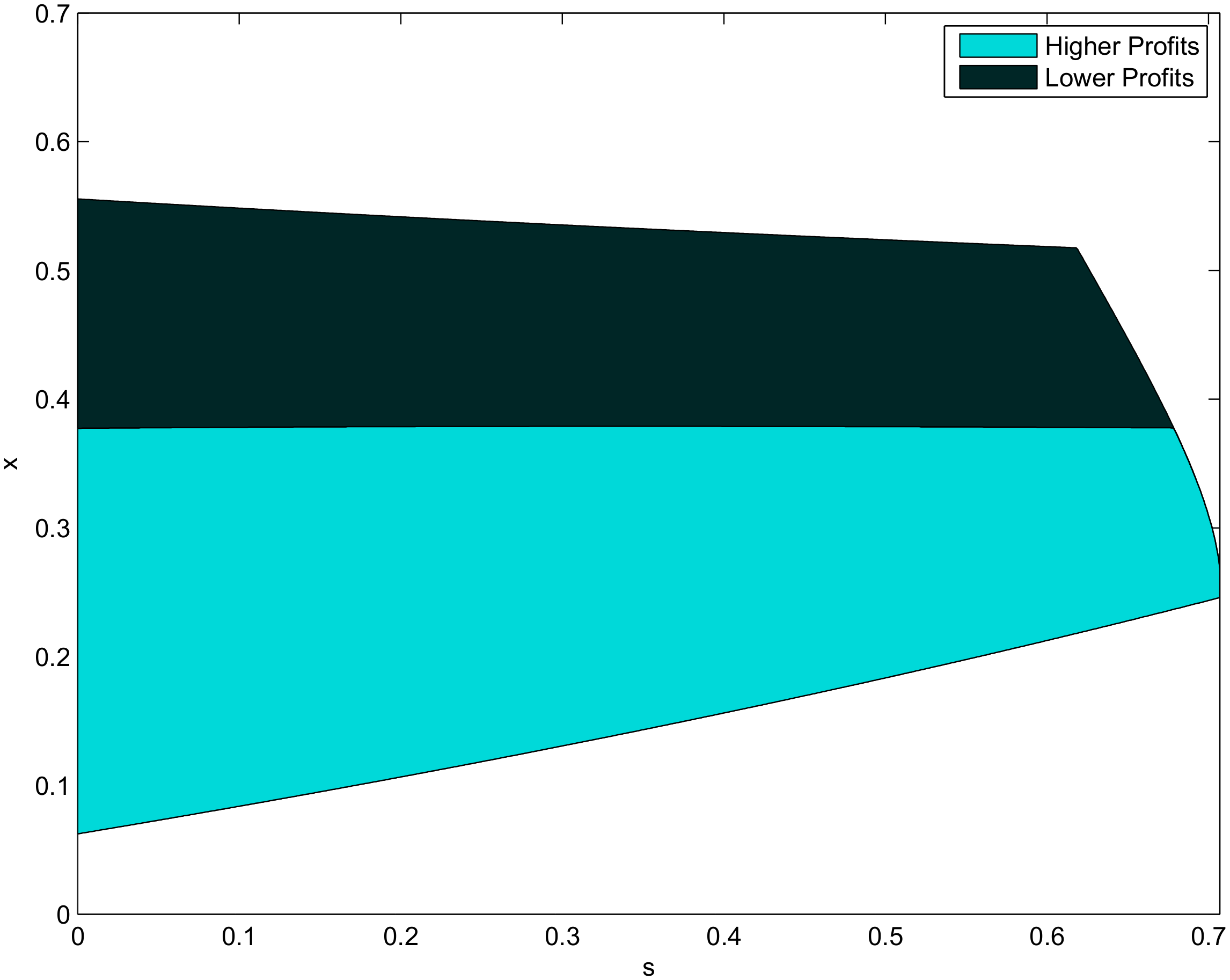
This result shows that, in the cost-dependent equilibrium, slight overconfidence can increase the profits of the overconfident player provided that cost asymmetries are sufficiently small. Figure 2 illustrates this by showing the relation between the ex-ante profits in the cost-dependent equilibrium with one overconfident player and one rational player and the ex-ante profits in the cost-dependent equilibrium with two rational players. The intuition is as follows. By making a mistake, the overconfident player has a “Stackelberg leadership gain” because it will produce at date 1 instead of date 2. However, the mistaken perception of the overconfident player will lead him to choose a quantity that is higher than the optimal one given his true cost. This leads to a loss which increases with the value of c since the difference between the optimal quantity and the quantity chosen increases with c. Hence, for sufficiently small values of c the “Stackelberg leadership gain” more than compensates the loss incurred by not playing the optimal quantity. For sufficiently high values of c, the reverse happens.

Proposition 3 also shows that overconfidence can lower the profits of the rational player. This happens because the mistaken perceptions of the overconfident player yield a reduction of market share for the rational player. If the rational player has low cost, then he produces at date 1. However, since the rational player knows that the overconfident player is likely to overproduce, the rational player must produce a smaller Stackelberg leader’s quantity than if he faced a rational opponent. If the rational player has high cost, then he produces at date 2. In this case, no matter if the overconfident player produces at date 1 or at date 2, the rational player will have a smaller market share than if he faced a rational rival.

Proposition 3.

(i) ${\Pi }_o\left(s\right)>\Pi \left(0\right)$ when $x\in \left[\omega \right(s),\tau (s\left)\right]$; (ii) ${\Pi }_o\left(s\right)<\Pi \left(0\right)$ when $x\in [\tau \left(s\right),\frac{5+s}{9+3s}]$; and (iii) ${\Pi }_r\left(s\right)<\Pi \left(0\right)$.

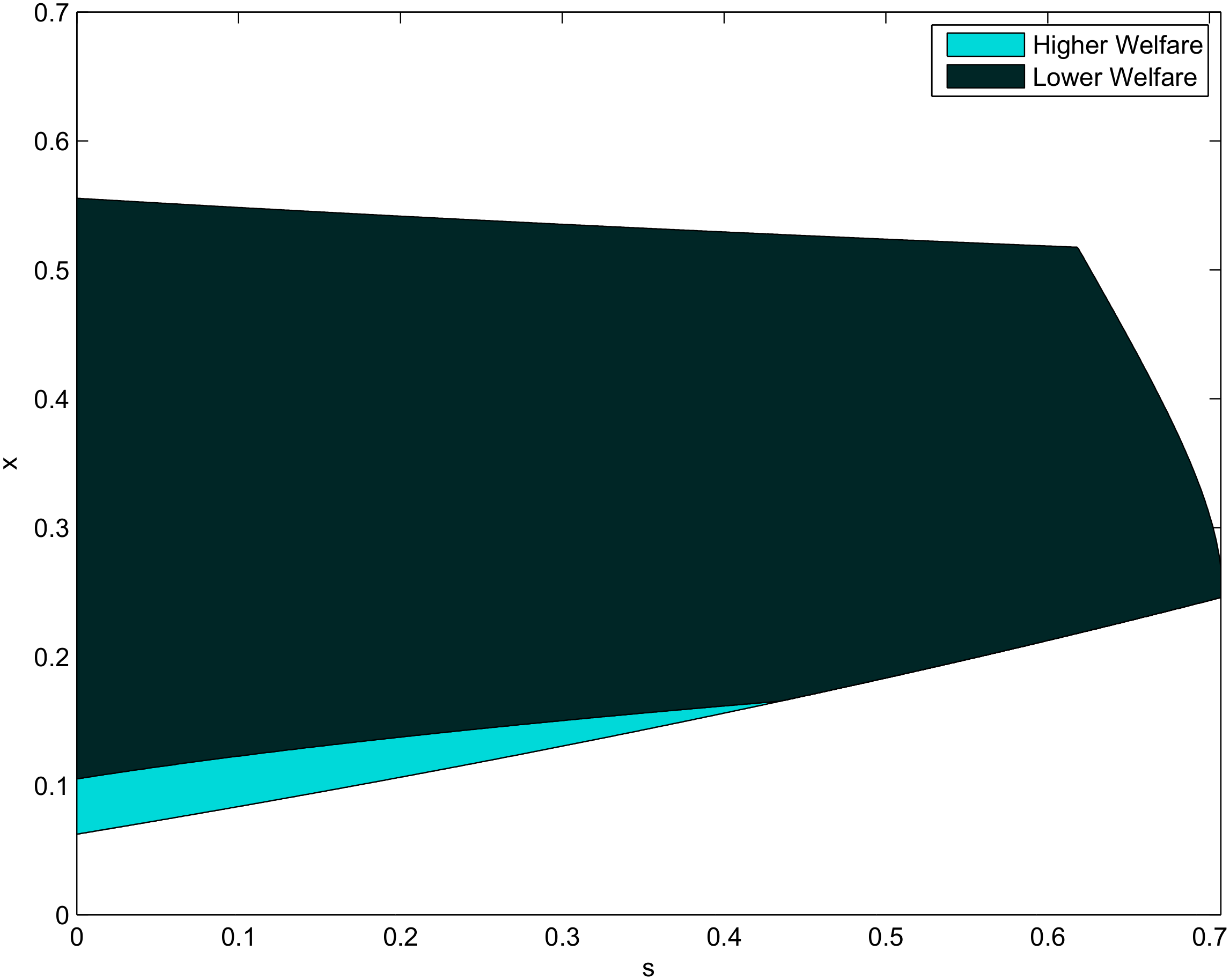
Our last result characterizes the impact of overconfidence on welfare (the sum of consumer and producer surplus). $W\left(s\right)$ denotes the ex-ante welfare in the cost-dependent equilibrium with an overconfident and a rational player. Let $W\left(0\right)$ denote ex-ante welfare in the cost-dependent equilibrium with two rational players .

Proposition 4.

(i) $W\left(s\right)>W\left(0\right)$ when $x\in \left[\omega \right(s),\psi (s\left)\right]$; and (ii) $W\left(s\right)<W\left(0\right)$ when $x\in (\psi \left(s\right),\frac{5+s}{9+3s}]$.

Figure 3 describes the relation between the ex-ante welfare in the cost-dependent equilibrium with one overconfident player and one rational player and the ex-ante welfare in the cost-dependent equilibrium with two rational players. Figure 3 shows us that slight overconfidence reduces welfare, except when cost asymmetries are sufficiently small. The intuition behind this result is as follows. Overconfidence increases the output of the overconfident player but reduces that of the rational player. The net effect is an overall increase in market output since the reduction in the output of the rational player is less than the increase in that of the overconfident player. The increase in market output raises consumer surplus but lowers producer surplus. It turns out that with slight overconfidence, the increase in the ex-ante profits of the overconfident player is less than the decrease in those of the rational player but with significant overconfidence the ex-ante profits of both players decrease. For sufficiently small cost asymmetries the increase in consumer surplus is of first-order and the reduction in profits is of second-order and so overconfidence increases welfare. When cost asymmetries are sufficiently high, the reverse happens and overconfidence lowers welfare.

5. Discussion

This section discusses some extensions of the model, its main assumptions, and limitations.

It would be straightforward to extend the model by assuming that costs can be $\underline{c}$ or $\overline{c}$ where $\overline{c}>\underline{c}>0$. The assumption that the prior probability is 1/2 could also be relaxed. This would complicate the algebra but it would not change the main findings of the paper.

It would also be straightforward to analyze a situation where both players are overconfident. In this case, the equilibrium strategies and beliefs of the two overconfident players would be qualitatively similar to the ones for the overconfident player described in Proposition 1. In such a situation, there would be a very high likelihood that both overconfident players commit at period 1 to high output levels. This would lower market price and industry profit but it would raise consumer surplus and welfare.

The analysis uses two main features of the model. First, that the profit function is continuous and concave. Second, that the first order conditions for profit maximization of a firm are linear in the quantities chosen by the other firm. The interesting question would then be to know to what extent the results generalize to other continuous and concave profit functions. The central result in this paper is based on payoff comparisons, involving strict inequalities. Therefore, the result must hold if the demand and the cost functions are such that the first order conditions for profit maximization are sufficiently close to linear on the other firm’s production. Nevertheless, the generalization of the result would require a different technique for the proof of the main proposition. The current one exploits the linearity of the best reply function, which is driven by the primitive assumptions on demand and costs.

6. Conclusions

In this paper, we characterize the impact of overconfidence on the timing of entry in a market, profits, and welfare. To do that we consider an endogenous timing model where players have private information about their cost, one of the players is rational but the other is overconfident. We find that, in a cost-dependent equilibrium, the overconfident player has a higher ex-ante probability of being the Stackelberg leader than the rational player. We show that this result is valid if and only if the overconfident player is slightly overconfident and cost asymmetries are intermediate. We also show that the overconfident player can be better off by being overconfident (although he does not know it) provided that cost asymmetries are sufficiently small. Finally, we show that overconfidence has an ambiguous impact on welfare since it increases consumer surplus while it reduces producer surplus. Our framework, therefore, provides a justification for the earlier entry of overconfident entrepreneurs and a motivation for firms hiring and retaining overconfident managers.

References

- Hamilton, J.; Slutsky, S. Endogenous timing in duopoly games: Stackelberg or Cournot equilibria. Games Econ. Behav. 1990, 2, 29–46. [Google Scholar] [CrossRef]
- Myers, D. Social Psychology; McGraw-Hill: New York, NY, USA, 1996. [Google Scholar]
- Dunne, T.; Roberts, M.J.; Samuelson, L. Patterns of firm entry and exit in U.S. manufacturing industries. RAND J. Econ. 1988, 19, 495–515. [Google Scholar] [CrossRef]
- Camerer, C.; Lovallo, D. Overconfidence and excess entry: An experimental approach. Am. Econ. Rev. 1999, 89, 306–318. [Google Scholar] [CrossRef] [Green Version]
- Malmendier, U.; Tate, G. CEO overconfidence and corporate investment. J. Financ. 2005, 60, 2661–2700. [Google Scholar] [CrossRef] [Green Version]
- Malmendier, U.; Tate, G. Does overconfidence affect corporate investment? CEO overconfidence measures revisited. Eur. Financ. Manag. 2005, 11, 649–659. [Google Scholar] [CrossRef]
- Galasso, A.; Simcoe, T. CEO overconfidence and innovation. Manag. Sci. 2011, 57, 1469–1484. [Google Scholar] [CrossRef] [Green Version]
- Hirshleifer, D.; Low, A.; Teoh, S. Are overconfident CEOs better innovators? J. Financ. 2012, 67, 1457–1498. [Google Scholar] [CrossRef] [Green Version]
- Branco, F. Endogenous Timing in a Quantity Setting Duopoly; Working Paper; Universidade Católica Portuguesa and CEPR: Lisbon, Portugal, 2008. [Google Scholar]
- Shao, X.; Wang, L. Manager’s irrational behavior in corporate capital investment decision-making. Int. J. Econ. Financ. Manag. 2013, 2, 183–193. [Google Scholar]
- Bénabou, R.; Tirole, J. Self-confidence and personal motivation. Q. J. Econ. 2002, 117, 871–915. [Google Scholar] [CrossRef]
- Lipsey, R.G.; Lancaster, K. The general theory of second best. Rev. Econ. Stud. 1956, 24, 11–32. [Google Scholar] [CrossRef]
- Albaek, S. Stackelberg leadership as a natural solution under cost uncertainty. J. Ind. Econ. 1990, 38, 335–347. [Google Scholar] [CrossRef]
- Van Damme, E.; Hurkens, S. Endogenous Stackelberg leadership. Games Econ. Behav. 1999, 28, 105–129. [Google Scholar] [CrossRef] [Green Version]
- Maggi, G. Endogenous leadership in a new market. Rand J. Econ. 1996, 27, 641–659. [Google Scholar] [CrossRef]
- Mailath, G. Endogenous sequencing of firm decisions. J. Econ. Theory 1993, 59, 169–182. [Google Scholar] [CrossRef]
- Normann, H. Endogenous Stackelberg equilibria with incomplete information. J. Econ. 1997, 66, 177–187. [Google Scholar] [CrossRef]
- Normann, H. Endogenous timing with incomplete information and with observable delay. Games Econ. Behav. 2002, 39, 282–291. [Google Scholar] [CrossRef]
- Van Damme, E.; Hurkens, S. Endogenous price leadership. Games Econ. Behav. 2004, 47, 404–420. [Google Scholar] [CrossRef] [Green Version]
- Malmendier, U.; Tate, G. Who makes acquisitions? CEO overconfidence and the market’s reaction. J. Financ. Econ. 2008, 89, 20–43. [Google Scholar] [CrossRef] [Green Version]
- Santos-Pinto, L.; de la Rosa, E.L. Overconfidence in Labor Markets. In Handbook of Labor, Human Resources and Population Economics; Zimmermann, K., Ed.; Springer: Berlin/Heidelberg, Germany, 2020. [Google Scholar]
- Zábojník, J. A model of rational bias in self-assessments. Econ. Theory 2004, 23, 259–282. [Google Scholar] [CrossRef]
- Benoît, J.-P.; Dubra, J. Apparent overconfidence. Econometrica 2011, 79, 1591–1625. [Google Scholar]
- Van den Steen, E. Rational overoptimism (and other biases). Am. Econ. Rev. 2004, 94, 1141–1151. [Google Scholar] [CrossRef] [Green Version]
- Santos-Pinto, L.; Sobel, J. A model of positive-self image in subjective assessments. Am. Econ. Rev. 2005, 95, 1386–1402. [Google Scholar] [CrossRef] [Green Version]
- Heifetz, A.; Shannon, C.; Spiegel, Y. The dynamic evolution of preferences. Econ. Theory 2007, 32, 251–286. [Google Scholar] [CrossRef] [Green Version]
- Heifetz, A.; Shannon, C.; Spiegel, Y. What to maximize if you must. J. Econ. Theory 2007, 133, 31–57. [Google Scholar] [CrossRef] [Green Version]
- Hyytinen, A.; Lahtonen, J.; Pajarinen, M. Forecasting errors of new venture survival. Strateg. Manag. J. 2014, 8, 283–302. [Google Scholar] [CrossRef]
- Cooper, A.; Dunkelberg, W.; Woo, C. Entrepreneurs’ perceived chances of success. J. Bus. Ventur. 1988, 3, 97–108. [Google Scholar] [CrossRef]
- Cassar, G. Are individuals entering self-employment overoptimistic? An empirical test of plans and projections on nascent entrepreneur expectations. Strateg. Manag. J. 2010, 31, 822–840. [Google Scholar]
- De Meza, D.; Southey, C. The borrower’s curse: Optimism, finance and entrepreneurship. Econ. J. 1996, 106, 375–386. [Google Scholar] [CrossRef]
- Brocas, I.; Carrillo, J. Entrepreneurial boldness and excessive investment. J. Econ. Manag. Strategy 2004, 13, 321–350. [Google Scholar] [CrossRef]
- Englmaier, F.; Reisinger, M. Biased managers as strategic commitment. Manag. Decis. Econ. 2014, 35, 350–356. [Google Scholar] [CrossRef]
- Vickers, J. Delegation and the theory of the firm. Econ. J. 1985, 95, 138–147. [Google Scholar] [CrossRef]
- Fershtman, C.; Judd, K.L. Equilibrium incentives in oligopoly. Am. Econ. Rev. 1987, 77, 927–940. [Google Scholar]
- Alvim, N.; Pires, T. Optimism and timing of market entry: How beliefs and information distortion create market leadership. Int. J. Econ. Theory 2017, 13, 289–311. [Google Scholar] [CrossRef]
- Squintani, F. Mistaken self-perception and equilibrium. Econ. Theory 2006, 27, 615–641. [Google Scholar] [CrossRef]
- Gervais, S.; Goldstein, I. The positive effects of biased self-perceptions in firms. Rev. Financ. 2007, 11, 453–496. [Google Scholar] [CrossRef] [Green Version]
- Santos-Pinto, L. Positive self-image and incentives in organisations. Econ. J. 2008, 118, 1315–1332. [Google Scholar] [CrossRef]
Figure 1.
Values of cost differences and overconfidence for which there exists a cost-dependent equilibrium. The shaded area includes all the values of cost differences—captured by the parameter x—and overconfidence—captured by the parameter s—for which there exists a cost-dependent equilibrium.
Figure 2.
Ex-ante profits of the overconfident player in the cost-dependent equilibrium versus ex-ante profits with two rational players. The figure reports the relation between the ex-ante profits of the overconfident player in the cost-dependent equilibrium and the ex-ante profits of a player in an endogenous timing game with two rational players for different values of x and s.
Figure 3.
Ex-ante welfare in the cost-dependent equilibrium with an overconfident player versus welfare with two rational players. The figure reports the relation between the welfare in the cost-dependent equilibrium with an overconfident player and the welfare in an endogenous timing game with two rational players for different values of x and s.
© 2020 by the authors. Licensee MDPI, Basel, Switzerland. This article is an open access article distributed under the terms and conditions of the Creative Commons Attribution (CC BY) license (http://creativecommons.org/licenses/by/4.0/).
Share and Cite
MDPI and ACS Style
Santos-Pinto, L.; Pires, T. Overconfidence and Timing of Entry. Games 2020, 11, 44. https://0-doi-org.brum.beds.ac.uk/10.3390/g11040044
AMA Style
Santos-Pinto L, Pires T. Overconfidence and Timing of Entry. Games. 2020; 11(4):44. https://0-doi-org.brum.beds.ac.uk/10.3390/g11040044
Chicago/Turabian StyleSantos-Pinto, Luis, and Tiago Pires. 2020. "Overconfidence and Timing of Entry" Games 11, no. 4: 44. https://0-doi-org.brum.beds.ac.uk/10.3390/g11040044
Note that from the first issue of 2016, this journal uses article numbers instead of page numbers. See further details here.