Biological and Chemical Control of Mosquito Population by Optimal Control Approach


Department of Mathematics, Universidad del Valle, Cali 760032, Colombia
*
Author to whom correspondence should be addressed.
†
These authors contributed equally to this work.
Games 2020, 11(4), 62; https://0-doi-org.brum.beds.ac.uk/10.3390/g11040062
Submission received: 12 November 2020
/
Revised: 7 December 2020
/
Accepted: 8 December 2020
/
Published: 14 December 2020
(This article belongs to the Special Issue Optimal Control Theory)
Abstract
:This paper focuses on the design and analysis of short-term control intervention measures seeking to suppress local populations of Aedes aegypti mosquitoes, the major transmitters of dengue and other vector-borne infections. Besides traditional measures involving the spraying of larvicides and/or insecticides, we include biological control based on the deliberate introduction of predacious species feeding on the aquatic stages of mosquitoes. From the methodological standpoint, our study relies on application of the optimal control modeling framework in combination with the cost-effectiveness analysis. This approach not only enables the design of optimal strategies for external control intervention but also allows for assessment of their performance in terms of the cost-benefit relationship. By examining numerous scenarios derived from combinations of chemical and biological control measures, we try to find out whether the presence of predacious species at the mosquito breeding sites may (partially) replace the common practices of larvicide/insecticide spraying and thus reduce their negative impact on non-target organisms. As a result, we identify two strategies exhibiting the best metrics of cost-effectiveness and provide some useful insights for their possible implementation in practical settings.
Keywords:
mosquito population dynamics; predator-prey system; chemical and biological control; optimal control; cost-effectiveness analysisMSC:
92D25; 49N901. Introduction
With the ongoing COVID-19 epidemics on the current agenda, both ordinary people and healthcare entities tend to neglect the prevention of other infectious diseases that are widely spread and persistent in the tropical and subtropical regions around the globe. Dengue fever, caused by four serotypes of the dengue virus (DENV1-4) is one of them, and more than 100 million symptomatic dengue infections occur every year with an average fatality rate of 0.5–1% [1]. Dengue virus is transmitted to human individuals through the bites of female mosquitoes that need to ingest human blood for maturing their eggs. One of the principal transmitters of dengue and other vector-borne infections is the invasive peridomestic species Aedes aegypti Diptera: (Culicidae) that has colonized all tropical and subtropical regions worldwide [2].
In the absence of an efficient vaccine or curative treatment [3], the most widely used approach to reduce human arboviral infections is the suppression of the vector population through the use of insecticides and larvicides. This method has been routinely applied in many tropical countries for decades, and the mosquitoes have developed a high degree of resistance to various chemical substances [4].
On the other hand, there are environmental concerns about the potential toxicity of larvicides and insecticides to non-target organisms, including the human population [5]. For this reason, the World Health Organization (WHO) and the Pan American Health Organization (PAHO) jointly promote and encourage the use of non-chemical strategies to control vector populations, highlighting the prominent role of biological control. In general terms, biological control is based on the use of “biological agents” (living organisms) that interact with mosquito populations through predation, competition, or parasitism [6,7].
In particular, natural enemies feeding on mosquito immature stages (principally, the younger larvae instars) can play an important role in suppression of local mosquito populations [8,9,10]. Indeed, mosquito larvae are preyed upon by different aquatic organisms including fish [11,12,13], amphibians [14,15,16], cyclopoid copepods [13,17,18], and even some aquatic insects [19]. Therefore, deliberate introduction of some predacious species in the known mosquito breeding sites may complement other vector control actions and contribute to suppression of local mosquito population. Therefore, the deliberate introduction of some predacious species in the acknowledged mosquito breeding sites may complement other vector control actions thus contributing to the suppression of the local mosquito populations. By naming the “acknowledged mosquito breeding sites”, we principally refer to the ornamental concrete and tiled bowls, basins, pools and other cavities filled with stagnant water that are surrounded by rich vegetation and form an essential part of the architectonic design of various tropical cities. Such ornamental basins can be found in various public places (e.g., shopping and recreational centers, parklands and clubs, residential complexes, open-air restaurants, school and university campuses, etc.) that account for people gatherings and congregations.
The primary goal of this paper is to design and analyze different short-term measures for the suppression of local mosquito populations based on various combinations of the traditional chemical control actions with the deliberate introduction of two possible types of predacious species bearing distinct features and to suggest the most cost-effective strategies for practical implementation. The secondary goal of this paper consists in finding out whether the biological control measures (namely, the presence of predacious species at the mosquito breeding sites) may replace the common practices of using chemical substances for suppression of local mosquito population and to what extent.
To achieve the goals stated above, we design a variant of the model developed in Reference [20] that accounts for two external control measures—application of larvicide and insecticide. These two substances induce additional mortality of the aquatic (immature) and aerial (adult) stages of A. aegypti mosquitoes and thus contribute to the suppression of their local populations. This model has a “local nature” meaning that it describes the population dynamics of A. aegypti mosquitoes in the surroundings of some breeding place represented by a single ornamental basin or an architectonic complex composed of several basins located nearby in some public areas with constant people flow or congregation. Here, it is worthwhile to recall that A. aegypti mosquitoes usually remain within a mean dispersal distance of 30 meters from their birthplace [21], which gives reasonable grounds to the model’s formulation.
Further, we employ the dynamic optimization approach in order to provide the formulation of our model in terms of the optimal control theory. To do so, we introduce the objective functional that synthesizes different purposes of the control intervention. On the one hand, the control actions seek to minimize the density of the adult mosquito population during the whole period of intervention, as well as the density of aquatic (immature) stages by the end of the intervention. On the other hand, it is also pursued to minimize the total quantity of chemical substances (larvicide and insecticide) during the control intervention.
In this context, it is worth highlighting that the optimal control technique provides powerful tools for design and comparative assessments of control strategies under diverse scenarios. For that reason, it has been widely used for the design and further analysis of intervention strategies based on mechanical, chemical, and biological control actions seeking the suppression of mosquito populations [22,23,24,25,26,27,28,29]. However, none of the published works explicitly address the optimal control applied to the dynamics of the mosquito population in the presence of natural predators feeding on mosquito immature stages. The present study intends to contribute to this strand of research by assessing the effect of predacious species on mosquito control under different scenarios.
A thorough description of the model fitting the optimal control modeling framework, as well as its core properties are presented in Section 2 of this paper, while Section 3 is devoted to the formal analysis of the formulated optimal control problem. In this section, we formally prove the existence of optimal controls, derive their characterizations by applying the Pontryagin maximum principle, and obtain the so-called optimality system consisting of six nonlinear ordinary differential equations (ODEs) with two-point boundary conditions.
Due to nonlinearity and the high dimension of the optimality system, its solutions can be found only numerically. Section 4 exhibits the outcomes of numerical solutions obtained by an advanced solver (GPOPS-II: Next-Generation Optimal Control Software, [30]) under diverse scenarios defined by different combinations of larvicides, insecticides, and predacious species. This section also contains the cost-effectiveness analysis of all designed strategies which is carried out using two different approaches for quantification of the effects (or benefits) of each strategy. Under the first approach, we only measure the capacity of each strategy for the suppression of local mosquito populations regardless of its environmental impact. Under the second approach, both the suppression potentials and eco-effects of all strategies are quantified. It is interesting to note that two different quantifications actually render dissimilar strategies as a result of the cost-effectiveness analysis. This issue is also discussed in Section 4 and some practical recommendations derived from the cost-effectiveness analysis are provided.
Finally, Section 5 resumes the highlights of this work and provides some useful insights for possible applications of our findings in practical settings.
2. Model Description
To describe the population growth of A. aegypti mosquitoes in the presence of natural predators of their immature stages, we employ the modeling framework proposed in Reference [20] and amend that model with two exogenous or control variables. Let denote the density of immature stages (eggs, larvae, pupae) effectively present at the moment t in some (ornamental) basin that contains stagnant water and can be viewed as a generic breeding site, and let define the density of female mosquitoes inhabiting the basin surroundings at the moment t. It is worthwhile to recall that urban domestic mosquitoes (such as A. aegypti) are weak flyers and they usually remain within a mean dispersal distance of 30 meters from their birthplace [21]. Therefore, the population size of male mosquitos (which is omitted in the model) is assumed similar to in order to guarantee that all females are able to mate successfully.
The model also includes a predator-prey interaction between the immature stages (prey) and a predacious aquatic species which is deliberately placed in the basin (breeding site). Moreover, in contrast to the original formulation given in Reference [20], the model we propose in this paper accounts for additional mortality for both mosquito states, and , which is attributed to spraying of larvicide and insecticide as an external measure of vector control. This control intervention is modeled by two control functions, and , denoting the spray rates of larvicide and insecticide spraying, respectively.
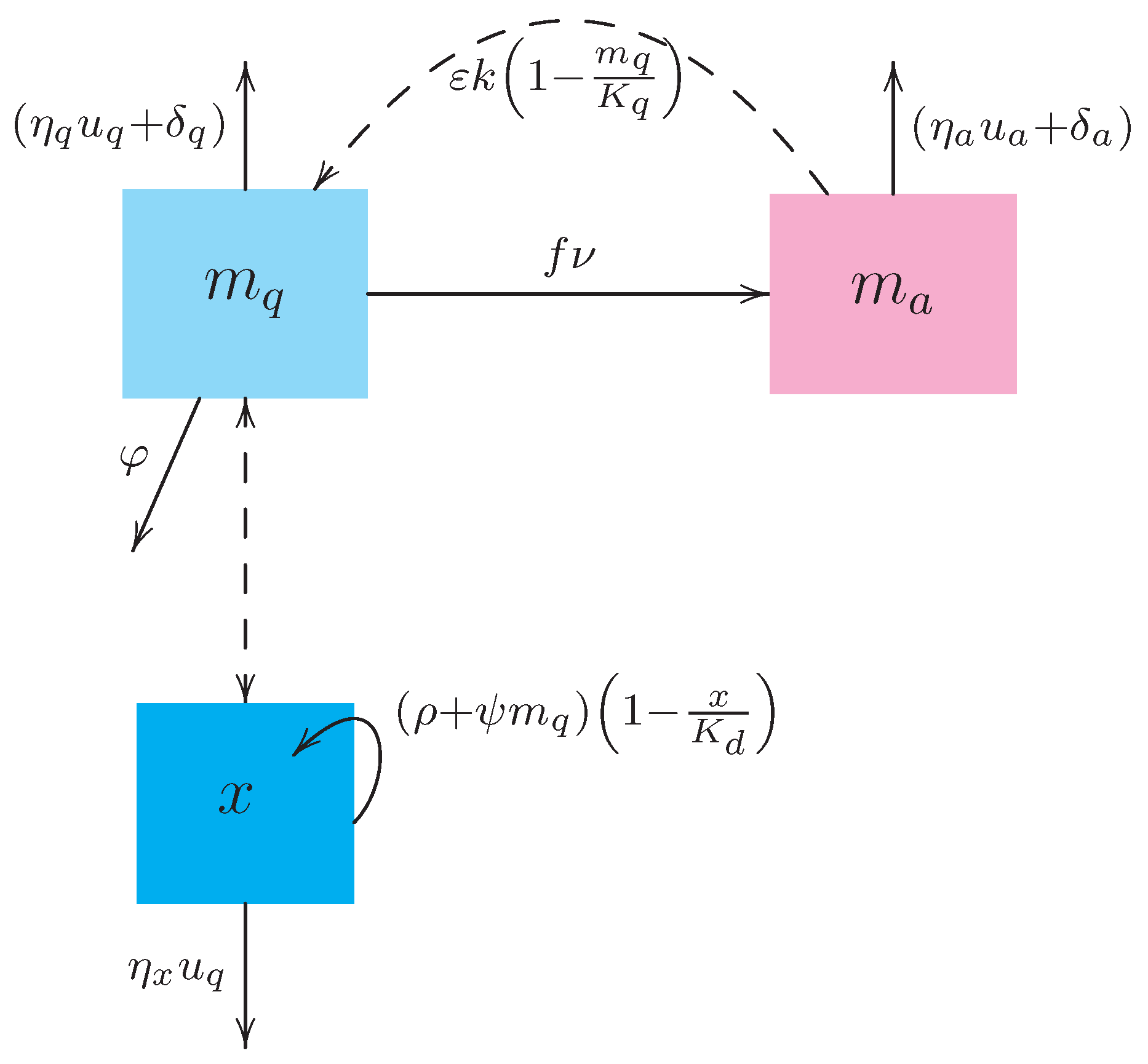
The mathematical formulation of the model involving control intervention results in the following dynamical system
with initial conditions
The flow diagram of the model (1) is presented in Figure 1 while the entries of the dynamical system are described in Table 1.
Equation (1a) states that immature stages (eggs, larvae, and pupae) are recruited due to the oviposition of adult female mosquitoes , the fraction of viable hatching eggs , the current density of female adult mosquitoes capable to laying eggs, and the remaining carrying capacity of the breeding site. The density of immature stages decays proportionally to their transition into adult stage , by natural mortality and by the larvicide application , and due to predation . Here, the predation rate is expressed using the “law of mass action” which is also known as Holling Type I functional response. Apart from trying to keep our model as simple as possible, this type of functional response assumes a linear increase in intake rate with prey density meaning that the time needed for chasing the prey is negligible. Such an assumption seems reasonable when a limited breeding site is considered and when the mosquito larvae (preys) rest on the water surface and constitute an easy target for predation.
It is also supposed that the predation of immature stages is carried out regardless of the prey gender; in other words, both male and female immature insects are apt for intake. Therefore, a fraction f of adult female mosquitoes is considered for the dynamics of and not for , in contrast to the model developed in Reference [31].
Equation (1b) expresses that the density of adult female mosquitoes increases by the transition of immature stages into adults that further become females . The population of decreases by natural mortality and by the insecticide application .
Finally, Equation (1c) states that the predacious species , deliberately introduced to the breeding site, exhibits logistic growth while its diet is not limited to the mosquito immature stages. The latter implies that has alternative food sources available in the basin (such as algae, ciliates, other insects and their immature stages, etc.). Therefore, the presence of (constituting an easy target) induces an additional increase in the predator’s intrinsic growth while the effect of the larvicide application () induces an additional decay of the predator density. This way of modeling is different from the standard application of the predator-prey models of Lotka-Volterra type where the predator species goes to extinction if there is no prey.
It was proved in Reference [20] that, in the absence of control intervention (), the trajectories of the system (1) belong to the invariant set
whenever . Furthermore, defined by (3) is an absorbing set of the system (1) with for all in the sense that all the trajectories of this system engendered by are attracted by .
It was also shown in Reference [20] that the basic offspring numbers of mosquitoes corresponding to the model (1) without control () have the following forms:
The above quantities Q and express the mean number of female mosquitoes produced on average by one female mosquito during her lifespan either in the absence or presence of the predacious species, respectively. It also holds that , which is in line with common sense.
Using the values of parameters of the model (1) without predacious species (, see also Table 2 ahead) estimated for the climatic conditions of the city of Cali, Colombia [32], it had been shown that for all temperature ranges. This explains durable persistence of the mosquito population in Cali, Colombia all the year around. On the other hand, from the expressions (4) one can relate the predatory efficiency (defined as ) with the entomological parameters of the mosquitoes and thus ensure that :
The inequality (5) states that the presence in the generic breeding site of a predacious species possessing a sufficiently high predatory efficiency may ensure local extinction of mosquito population at the long run. In other words, with (5) in force, it is guaranteed that one female mosquito produced on average less than one female mosquito as a result of predatory efficiency of .
However, it seems very demanding to find a particular species of predators bearing the biological characteristics and that fulfill the relationship (5). Therefore, the introduction of in a generic breeding site should be combined with other vector control measures in order to render the desired outcome of either drastic reduction of the mosquito population in the surroundings of the basin or its local extinction.
The traditional method for reduction of local mosquito populations relies upon application of chemical control measures, such as spraying of larvicides and insecticides. From the mathematical standpoint, these control measures induce an increase in the parameters and denoting natural mortality rates of immature and adult insects. The effect of the chemical control measures on the basic offspring numbers Q and can be assessed using the so-called normalized forward sensitivity indexes of Q and with respect to and . According to the definition given in Reference [35], the normalized forward sensitivity indexes admit the following values:
From the above relationships, we can clearly see that Q and exhibit higher sensitivity to the insecticide control (acting upon ) than larvicide control (acting upon ). For example, using the definition given in [33], if the natural mortality of adult mosquitoes is increased by 20% due to the insecticide spraying, the values of Q and will be reduced by . On the other hand, if the natural mortality of immature insects is increased by 20% due to the larvicide spraying, the values of Q and can be reduced only by and , that is, less than by 16.67%.
Remark 1.
Since , the action of larvicide may seem more noticeable in the absence of predacious species than in their presence. Bearing in mind that , it is worthwhile to recall that a function of the form with has a steeper descent for smaller (positive) values of than for larger values where remains unchanged.
Note that the right-hand sides of the system (1) are decreasing with respect to the control variables and . Therefore, the trajectories of the system (1) with engendered by any initial condition remain in for all . In other words, the dynamical system (1) remains well-posed for all non-negative and bounded piecewise continuous control functions and . Moreover, in the presence of chemical control actions one may expect the reduction of the basic offspring numbers (4) determined for the system (1) without control intervention.
Let be the finite period of time corresponding to control intervention which is modeled by two piecewise-continuous control functions
where the positive constants and define the maximum rates for daily application of larvicide and insecticide, respectively.
The purpose of the control intervention is multi-objective and can be determined by the following objective functional
to be minimized with respect to and satisfying the condition (7) under dynamical constraints imposed by the system (1) with given initial conditions (2). In the above expression, the non-negative constants and stand for the weight coefficients and define the priorities of decision-making associated with each single objective. Namely, the terminal term of (8) expresses the minimization of the density of immature stages by the end of control intervention (at ). The first term in the integrand of seeks to minimize the total number of adult females (capable of transmitting arboviral infections) during the whole period of control intervention, while the last two terms in the integrand of (8) are related to the minimization of the control effort. Here, we assume that there is no linear relationship between the coverage of control interventions and their underlying costs; therefore, the integrand function is quadratic with respect to both control functions. This assumption is wildly used in dynamic optimization dealing with chemical measures of vector control [27,28,29], and this issue is also addressed in Remark 2 (see Section 3 ahead).
3. Existence of Optimal Controls and Their Characterizations
The model described in the previous section can be formulated as a standard problem of optimal control with fixed time of control intervention. Let
be the set of admissible controls, where represents the set of piecewise continuos functions on . Then the optimal control problem can be posed as follows. Find a pair of control functions such that
subject to the dynamic constraint defined by the system (1) with initial conditions (2).
The optimal control problem formulated above can be directly solved by applying the Pontryagin maximum principle (see Reference [36] or similar textbooks for more details) which constitutes the necessary condition of optimality. However, the existence of optimal controls satisfying (10) should be formally established prior to the application of this necessary condition. For this purpose, we formulate the following statement.
Proposition 1
Proof.
To prove the existence of satisfying (10), we employ the classical approach based in the Filippov-Cesari existence theorem thoroughly described in References [37,38]. To apply this theorem, we have to show that our optimal control problem (10) subject to (1), (2), and (9) fulfills a series of conditions that are sufficient for the existence of an optimal solution:
- (i)
- (ii)
- The sets of all initial and terminal states and are closed and bounded in .
- (iii)
- For each , the control functions take values from the closed, bounded, and convex set .
- (iv)
- The right-hand sides of the dynamical system (1) are linear with respect to the control functions .
- (v)
- The termuinal-state function in the objective functional (8) is continuous in its arguments.
- (vi)
- The integrand of (8) is convex in and satisfies the coercivity conditionwith some constants and .
Items (i)–(ii) have been already corroborated in Section 2. Namely, it was established that dynamical system (1) has a unique solution that exists for all and for any . Moreover, if this solution is engendered by the initial condition then for all . Furthermore, if is engendered by the initial condition then we have that
since (defined by (3)) is an absorbing set of the dynamical system (1) when and the right-hand sides of (1) are decreasing with respect to the control variables and .
The credibility of items (iii)–(v) is beyond doubt, while item (vi) is fulfilled with and This completes the proof. □
The optimal solution of the problem (10) (that exists in virtue of Proposition 1) and the corresponding solutions of the dynamical system (1) with assigned initial conditions (2) must satisfy the necessary condition of optimality expressed by the Pontryagin maximum principle [36]. Generally speaking, the maximum principle allows to convert the minimization (resp. maximization) of the objective functional with respect to on the functional set (9) into the point-wise minimization (resp. maximization) of a scalar function (known as Hamiltonian) with respect to variables and almost for all along the optimal trajectory . For our optimal control problem, the Hamiltonian is defined as
where can be viewed as a vector of Lagrange multipliers linked to the differential constraint expressed by the system (1). On the other hand, are time-varying real adjoint functions that express the marginal variations in the value of objective functional induced by changes in the current values of state variables (in the “component-by-component” sense). In other words, the current values of reflect additional benefits or costs associates with changes in and they are necessary elements of the Pontryagin maximum principle [36]. Namely, they are solutions to the following adjoint ODE system
with transversality conditions
Proposition 2
(Characterizations of optimal controls). Let be a pair of optimal control that fulfills (10) and let , , denote the corresponding solutions of the dynamical system (1)–(2) defined for . Then there exists a piecewise differentiable adjoint function satisfying (12)–(13) such that
and almost for all . Furthermore, the optimal controls and admit the following characterizations:
Proof.
If the optimal pair fulfills the condition (10) then this pair of controls must also comply with the necessary condition of the Pontryagin maximum principle which is , that is,
In other words, the Hamiltonian (11) must have a critical point in . Furthermore, it is easy to check that
is positive definite; therefore, the Hamiltonian attains its minimum with respect to u at and the relationship (14) takes place.
Remark 2.
It is worthwhile to recall that the necessary conditions (16) have conceptual interpretations from the economics standpoint. Namely, they imply that, under optimal control strategies and at each , the marginal costs of control actions (expressed by the terms and , respectively) must be equal to their marginal benefits (given by the terms and , respectively). This is exactly what is displayed in the middle rows of (17) and (18).
In view of Proposition 2, the optimal control problem, that consists in minimization of the objective functional (8) on the set of admissible controls (9) and subject to the dynamical system (1) with initial conditions (2), can be reduced to the solution of two-point boundary value problem which is usually referred to as optimality system [36]. The latter is composed of six ODEs given by (1) and (12) where the control functions and are replaced by their characterizations (15), plus two sets of boundary conditions: three initial conditions (2) specified at and three transversality conditions (13) defined at .
In this context, it is worthwhile to note that the existence of the optimal controls (proved in Proposition 1) implies solvability of the optimality system. Moreover, using some conventional techniques [39,40], the uniqueness of the solution of the optimality system can also be established for sufficiently short intervals of time when the right-hand sides of the optimality system are Lipschitz-continuous with respect to all state and adjoint variables. This condition is fulfilled for the right-hand sides of (1) and (12) where the control functions and are replaced by their characterizations (15). Therefore, it is plausible to suppose that the optimality system is well-posed for sufficiently short periods of time, and has a unique solution.
It is also understood that, due to the high dimension and nonlinearity of the optimality system, its solution can only be found numerically, and in the next section we present and analyze numerical solutions corresponding to different scenarios.
4. Numerical Solutions under Different Scenarios
4.1. Preliminary Settings
In accordance with estimations performed in Reference [32] for average daily temperature (23.9 °C) in the city of Cali, Colombia, and other data found in scientific literature, Table 2 displays numerical values assigned to all constant parameters of the dynamical system (1) which will be kept unaltered during the computational experiments involving numerical solutions of the optimal control problem (10).
It is worth noting that, for parameter values from Table 2, the basic offspring number defined by (4a) is meaning that one female mosquito produces on average 38 female mosquitoes in the absence of predacious species. This value matches the estimations of the basic offspring number obtained in other studies [41].
A shallow basin we consider here has the volume of about 100 liters, and a maximal larval density is 8-10 individuals per liter [34] what gives us the carrying capacity (measured in thousands of individuals). We also assume the following stylized values related to the predacious species
where (measured by the maximal number of individuals to be sustained by the environment) is defined to match the predator-prey ratio in accordance with [42]. To assume an abundance of immature and adult mosquitoes before the control intervention, we define and and also consider two options for with expressing the absence of predacious species during the control intervention, and mimicking the introduction of three individuals (one male and two females) into the basin before the control intervention.
For all numerical experiments, we set meaning that the control intervention will remain in force during 30 days.
To perform numerical simulations we have employed the next-generation optimal control software package GPOPS-II1 designed for MATLAB platform [30] that implements an adaptive combination of direct and orthogonal collocation techniques known as Radau pseudospectral method [43].
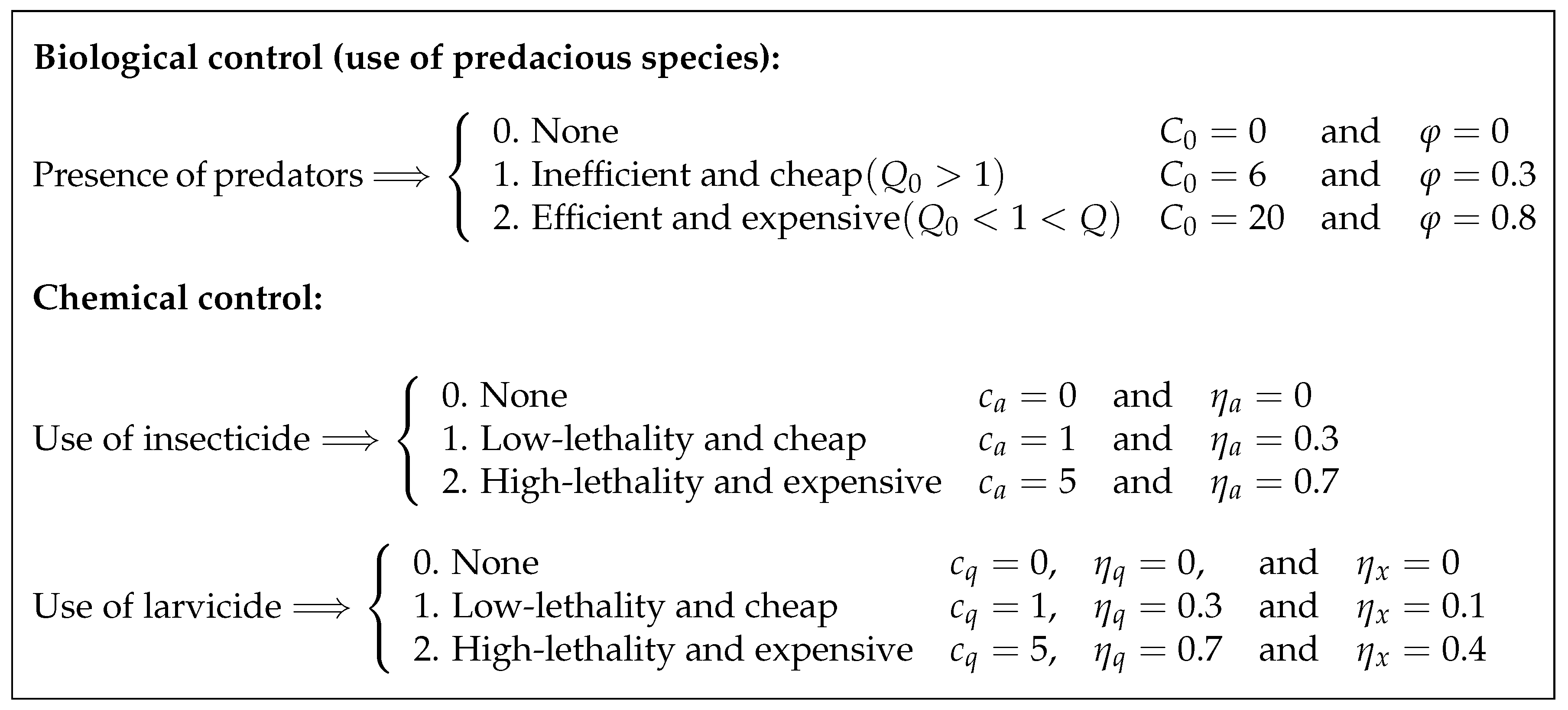
Our goal is to analyze different scenarios, whose determination results from the following considerations. First, there are scenarios where the biological control is either absent () or present (). For the latter, we perform testings with two predacious species—one that is relatively cheap but does not fulfill the condition (5) of predatory efficiency (to be referred further as inefficient or inert predator), and another that fulfills the condition (5) but comes at a higher cost (to be called efficient or aggressive predator in the sequel). The unit cost (i.e., per individual) for both types of predacious species is denoted by . As stated in Reference [13], different larvivorous fish species constitute an example of inefficient or inert predators, while cyclopoid copepods are usually regarded as aggressive and efficient ones.
Second, there are scenarios either accounting or not for the chemical controls actions applied to adult insects only (insecticide spraying) or their immature stages only (larvicide spraying), or to both mosquito populations (combined use of insecticides and larvicides). Additionally, we consider two types of each chemical substance: one bearing high lethality and costs, and another bearing low lethality with moderate underlying costs.
In this context, it is worth recalling that the lethality of existent insecticides and larvicides admits variation between 20% and 80% [44,45,46]; therefore, we suppose 30% efficiency for low-lethality substances and 70% efficiency for high-lethality substances. Such efficiencies are modeled by the parameters (for insecticides) and (for larvicides) in the dynamical system (1), while the underlying (unit) costs of larvicide and insecticide are expressed, respectively, by and in the objective functional (8). Furthermore, we assume that the upper bound of both control functions are normalized to unity: . The latter implies that the daily use of each chemical substance cannot exceed certain quantities and determined externally by the environmental regulations, that is,
Thus, and are the fractions of and to be used at each day of the chemical control intervention, and therefore . Note that the quantities and may have different values for larvicides and insecticides bearing lower or higher lethality; this is another reason why we have introduced normalization for and .
We also assume that the negative effect of larvicides on the predacious species (expressed in (1) by the parameter ) increases with the larvicide’s lethality.
Finally, since our primary goal is to suppress the total mosquito population (and thus reduce the local incidence of dengue and other vector-borne diseases), in the integrand of the objective functional (8), we assign the highest value to the weight coefficient . Thus, doubles the unit cost of the most expensive chemical control. As for the weight coefficient accompanying the terminal part of (8), we set to make it the largest and also offset the T days of intervention.
4.2. Description of Considered Scenarios
In the previous subsection, we assigned numerical values to the majority of the constant parameters of the optimal control problem (10) which will be kept unaltered during the computational experiments. However, numerical values for several parameters (namely, for and ) have not been determined yet. These are exactly the parameters whose values will be varied in order to express different scenarios and to obtain the optimal strategies corresponding to each particular scenario.
Altogether, we intend to explore 27 scenarios and to establish 27 corresponding strategies (schematically displayed in Figure 2) which are further codified using three digits ( and 2) referring to the use of predacious species (first digit) for biological control, use of insecticide (second digit) on the adult population, and application of larvicide (third digit) on immature stages. Thus, the strategy denoted by 012 implies no use of predacious species and application of low-lethality insecticide in combination with high-lethality larvicide, while the strategy 000 corresponds to the absence of control intervention and will be referred to as “baseline case” in the sequel. Figure 3 presents the profiles and corresponding to the baseline case (Strategy 000).
It is worthwhile to point out that we do not have any reliable information regarding the unit costs of insecticides and larvicides bearing different lethalities. Therefore, in view of the rationale given in References [28,29], the values assigned to the weight coefficients and (as displayed in the chart of Figure 2) are taken only for the purpose of theoretical analysis; for practical purposes, these values should be adjusted to more realistic ones.
To characterize performance of each strategy, we evaluate the following important quantities for each run of GPOPS-II solver feeded diverse combinations of values as indicated in Figure 2:
- The density of immature stages at the end of the intervention:
- The cumulative density of adult females during the whole period of intervention: .
- Cumulative fraction of larvicide used:
- Cumulative fraction of insecticide used:
- The total cost of the strategy that combines expenses related to the initial introduction of a predacious species and the costs of chemical control measures, that is,
In the above expressions, denote the optimal states of the system (1) corresponding to the optimal controls delivered by the GPOPS-II solver under different scenarios described in Figure 2. It is worthwhile to point out that the baseline case (Strategy 000) and two scenarios not relying upon the use of chemical substances (Strategies 100 and 200) do not require for numerical solutions of the optimal control problem (10). Therefore, to obtain and corresponding to Strategies 100 and 200 it suffices to solve numerically the system (1) with and .
The outcomes displayed in Table 3 plainly indicate that Strategy 001 is the cheapest, while Strategies guarantee the best results for suppression of the total mosquito population by the end of the control intervention. Among them, Strategy 220 does not require the use of larvicide and thus bears a lower total cost, while Strategy 221 appears a bit cheaper than Strategy 222 and requires a lesser amount of insecticide.
Note that for the baseline case (Strategy 000) we have
while its underlying cost is zero since no control action is applied.
Now, we are interested in determining which strategy or strategies may serve better the needs of the decision-makers. In order to proceed, we have to assess and quantify the benefits rendered by each strategy in order to employ the so-called cost-effectiveness approach to the result of numerical solutions of the optimal control problem in the sense of References [28,47]. In the following subsection, we perform the cost-effectiveness analysis of the strategies displayed in Table 3.
4.3. Cost-Effectiveness Analysis
In economics, the cost-effectiveness analysis is the method that allows comparing the relative costs and outcomes (effects or benefits) of different courses of action. Using this approach, one can fairly assess an additional benefit that can be obtained by investing a unit of cost into a certain action in comparison to either no action taken or implementing a different action.
To employ this approach, it is necessary to quantify the relative costs and benefits of each strategy that models an external intervention. The relative costs of control strategies described by 27 scenarios given in Figure 2 can be assessed by (see Formula (19) and the last column of Table 3), while some additional considerations will be needed to quantify the benefit of each strategy.
First, let us recall that the primary goal of the control intervention consists in minimizing the density of immature stages by the end of the intervention (cf. terminal term in (8)) and reducing the density of adult mosquitoes during the whole period of intervention (cf. first summand of the integrand in (8)). Therefore, the effect of each strategy on the suppression of mosquito population can be quantified as
where and are defined by (20) in regards to the baseline case (that is, without control intervention, ) while and correspond to the optimal states of the dynamical system (1) for each optimal strategy (cf. first column of Table 3).
The secondary goal of the decision-making (expressed by the last two summands of the integrand in (8)) consists of minimizing the use of larvicide and insecticide since these chemical substances may have an adverse environmental effect besides generating additional costs. Therefore, we would also like to identify a strategy (or strategies) capable of reducing the mosquito population with a relatively low impact on the environment. To do so, it is plausible to assume that the negative environmental impact of these chemical substances is proportional to their quantities used for the strategy’s implementation. Let us recall that the maximal quantity of the larvicide (resp. insecticide) allowed to be used at each day of control intervention is (resp. to ). Therefore, the maximum amounts of both chemicals allowed to be used during the period of control intervention cannot exceed and , respectively. By assuming that the quantities of larvicide and insecticide are directly related to their adverse effects on the environment, one may consider as an additional ecological benefit of each strategy the relative quantity of each chemical which is not spent during the period of intervention. Under this setting, the eco-effect of each strategy can be quantified as
It is worth noting that, according to the above formula, the highest possible eco-benefit is assigned to two strategies (coded as 100 and 200) that do not require the use of chemical substances. The combined effect of each particular strategy can be then defined as a sum of and leading us to the following formula
Once the relative costs and effects are defined for each strategy, the cost-effectiveness analysis can be performed. One of the main indicators frequently used in this type of analysis is the so-called “Average Cost-Effectiveness Ratio” (or ACER) that expresses the average cost related to obtaining one unit of potential benefit by employing the underlying strategy [28,47]. In formal terms, ACER is the ratio of the cost to benefit of a particular control action in comparison to no action (i.e., baseline case), that is
where “Strategy X” can be replaced by one of the coded strategies given in the first column of Table 3. Note that the costs corresponding to all considered strategies 001-222 are already quantified as by means of the formula (19) and their underlying values are given in the last column of Table 3.
According to (24), smaller values of ACER indicate higher efficiency of the control action in the sense that one unit of potential effect (or benefit) comes at a lower cost. Table 4 displays the effects quantified by Formulas (21) and (23) together with underlying values of two ACER types evaluated for all strategies 001-222. In particular, ACER (column 4 in Table 4) gives the average cost-effectiveness ratio that only encompasses the effect of each strategy on the suppression of mosquito population, whereas ACER (last column in Table 4) also accounts for the eco-effect of each strategy.
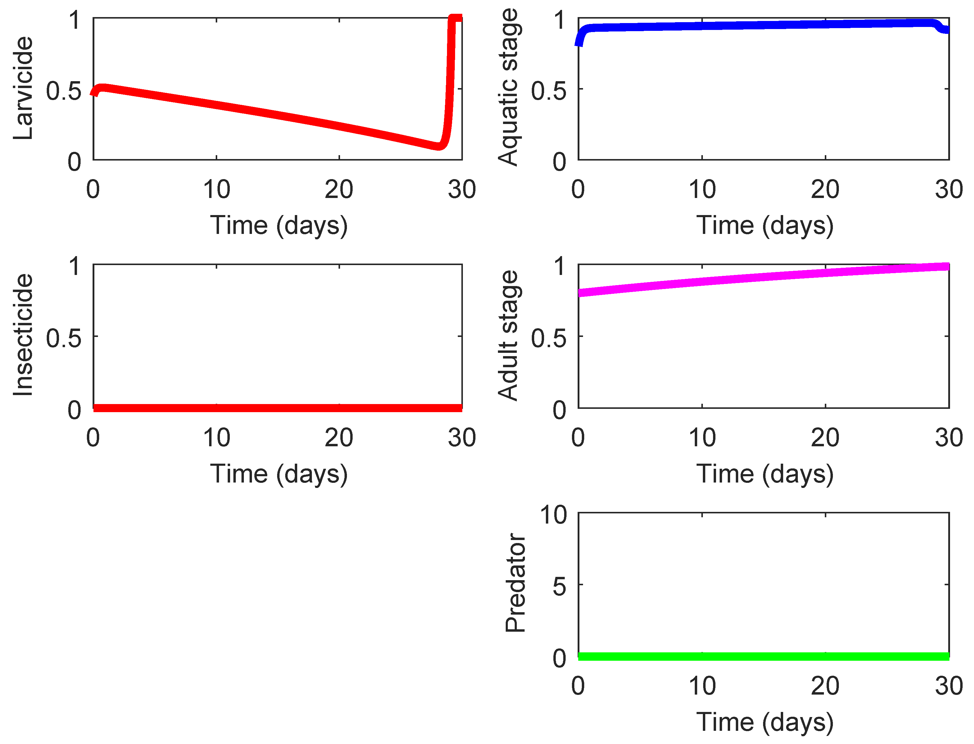
According to the total costs invested in the control intervention (see the first column of Table 4), the cheapest strategy is the one coded as 001 (application of low-lethality larvicide in the absence of the predacious species, see Figure 4); however, its effect on suppression of the mosquito population, , is also the lowest comparing to other strategies. As shown on the left upper chart of Figure 4, this strategy requires a moderate use of low-lethality larvicide (that is relatively cheap) during the major part of the control intervention ( and the application of the maximum quantity of the larvicide during the last two days ().
From the practical standpoint, this modus operandi evokes some doubts since the profiles of both mosquito populations and corresponding to Strategy 001 bear little difference from the uncontrolled case (baseline strategy, cf. Figure 3), except for the last two days where a “strong action” is put in place. The latter is done as an attempt to minimize the terminal term of the functional (8) to compensate for a rather weak effect of this strategy on the reduction of mosquito population. It is also worth noting that Strategy 001 requires for a relatively small amount of larvicide and does not require the use of insecticide. Due to this and the lowest cost, the average cost-effectiveness ratio of this strategy accounting for its eco-effect, ACER, also exhibits the best result in comparison to other strategies.
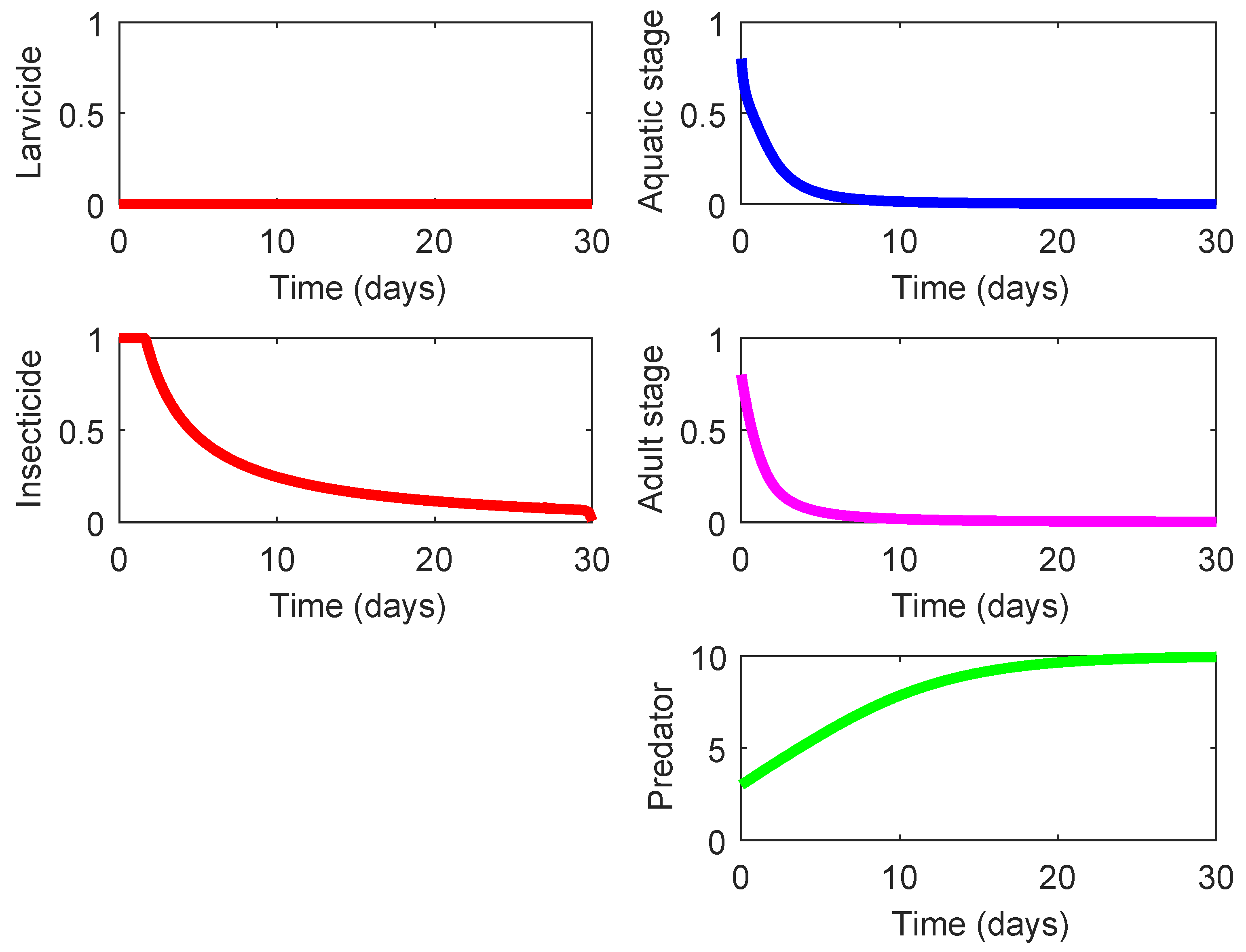
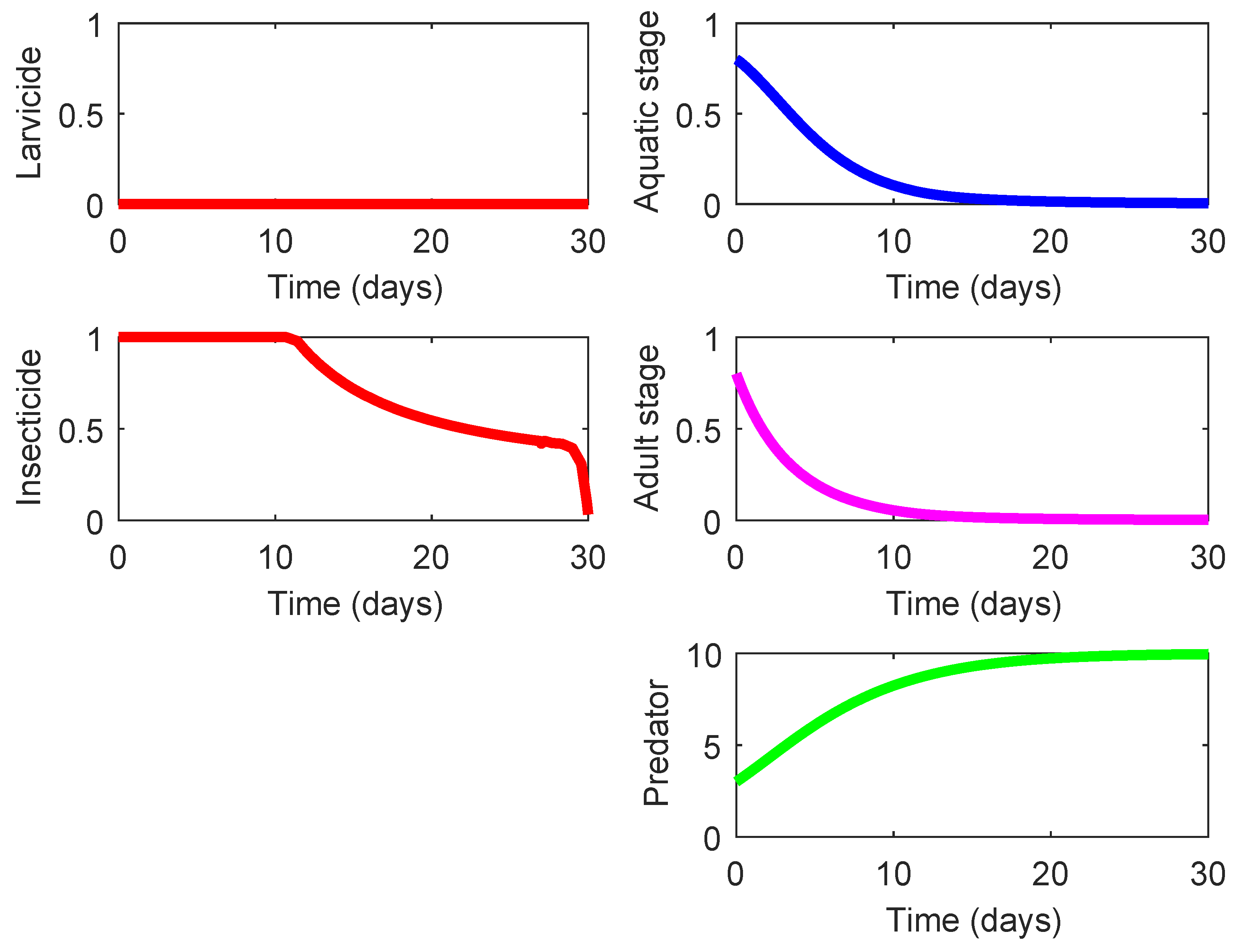
The last three rows in Table 4 display three strategies (Strategies 220, 221, and 222) that demonstrate the highest effect on suppression of the mosquito population and also exhibit a notable eco-effect. Among them, Strategy 220 (consisting in the use of high-lethality insecticide in the presence of efficient predacious species, see Figure 5) possesses a slightly higher of ACER since this strategy does not require the larvicide spraying unlike the other two strategies. As shown in Figure 5, the presence of some efficient predacious specie combined with a moderate spraying of high-lethality insecticide guarantees steady decline of both mosquito population. The results for Strategies 221 and 222 are very similar to those presented in Figure 5, and they are omitted here. The only difference is exhibited by the nonzero control profile according to which the larvicide spraying should by employed (at a moderate mode) during the last couple of days in order to ensure the minimization of the terminal term in the objective functional (8).
It should be pointed out that, besides rendering the best effects, Strategies 220, 221, and 222 also involve significant costs (10-times higher than the cost of Strategy 001), and for that reason, their ACER values are considerably larger than for other strategies.
In this context, one can easily detect in Table 4 that Strategy 110 (consisting of spraying of low-lethality and cheap insecticide in the presence of inefficient or inert predacious species, see Figure 6) exhibits the best value of ACER related to the suppression of the mosquito population. As shown in Figure 6, Strategy 110 requires to use a considerable amount of low-lethality insecticide that should be sprayed at the maximum daily rate during the first 12 days of control intervention, with a gradual reduction for the consequent 17 days, followed by total suspension at the end of intervention period. For that reason, the value of ACER corresponding to the Strategy 110 is greater than for other strategies that require a smaller total amount of chemical substances.
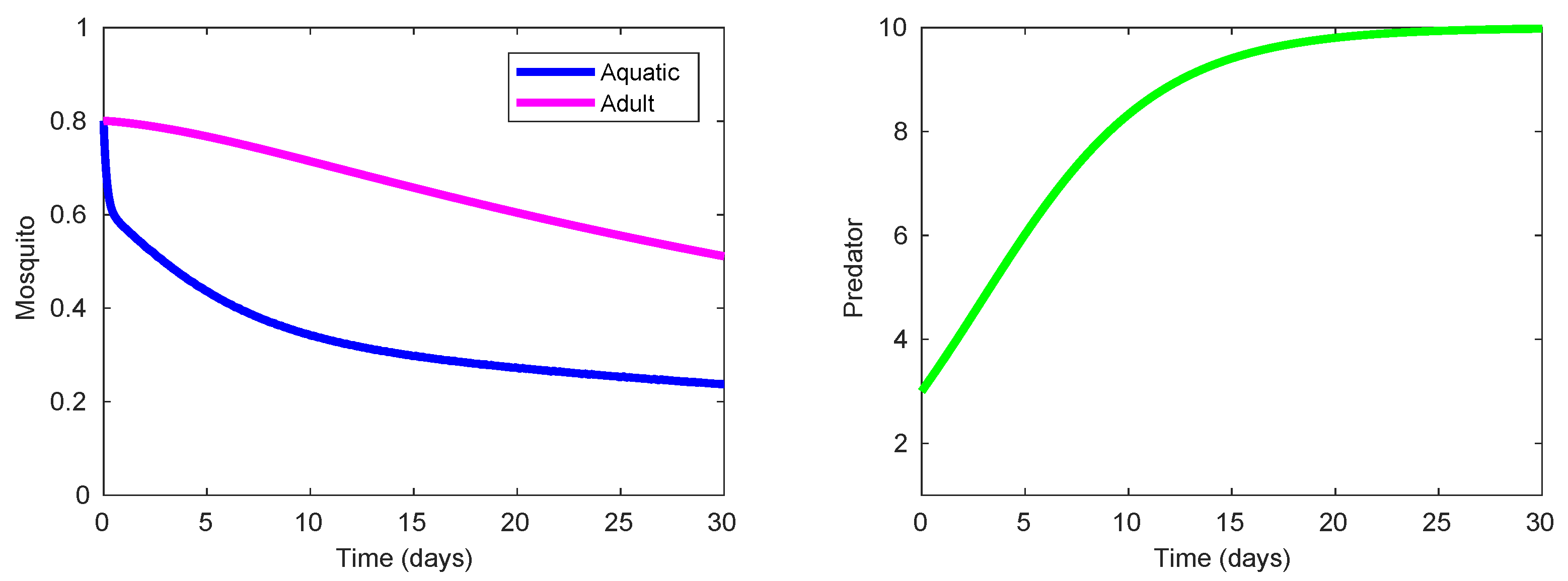
We have already mentioned that the cheapest strategy (Strategy 001, see Figure 4) is the one rendering the smallest benefit with regards to the suppression of the mosquito population. By revising the second column of Table 4, we can identify that Strategy 100 (see Figure 7 is also relatively cheap but its corresponding effect is almost 10 times greater that that of Strategy 001. Moreover, Strategy 100 is eco-friendly because it does not require the use of chemical substances ( and ). For that reason, its average cost-effectiveness ratio ACER that accounts for the eco-effect is the lowest besides the ACER for Strategy 001.
Using the values of ACER (see the fourth and last columns in Table 4) one can fairly assess the cost to be invested in each intervention strategy for obtaining one unit of the corresponding effect or benefit in comparison to the baseline case (i.e., no intervention and zero cost). On the other hand, it seems also useful to compare mutually exclusive strategies with each other.
For this purpose, there is another standard indicator which is known as Incremental Cost-Effectiveness Ratio (or ICER). This indicator is defined by the difference in cost between two possible interventions, divided by the difference in their effect [28,47]. The value of ICER represents the average incremental cost associated with one additional unit of the measure of effect when two mutually exclusive strategies are compared. The value of ICER can be estimated as
and its calculation starts with the cheapest strategy. Thus, the value of ICER measures an additional cost per unit of additional outcome (effect or benefit) when the current Strategy X (bearing lower costs) is replaced by a new Strategy Y which is more expensive but renders a more notable effect.
In the first instance, let us calculate ICER for Strategies 001-222 taking into account only their effects on the suppression of mosquito population, . The initial step is to arrange all strategies in ascending order regarding their costs and effects (given in the second and third columns in Table 4). Strategies that do not comply with this order should be removed. The results are given in Table 5 where Strategies 002, 011-022, 111-112, and 200-212 have been tossed out as non-abiding to the above-stated rule. Note that the cheapest strategy (in our case, Strategy 001) is compared with the baseline case (Strategy 000 without control intervention) and, therefore, its ICER coincides with its ACER.
The next step consists of eliminating all strategies whose ICER-values do not comply with ascending order, as well as those with indefinite ICER (i.e., strategies having ). For the set of remaining strategies, the values of ICER are calculated again according to (25) until there are no more strategies to be removed. Note that the lowest ICER-value in the last column of Table 5 corresponds to Strategy 110. Therefore, all strategies that standing above Strategy 110 in Table 5 should be removed. As a result, we obtain the list of potentially cost-effective strategies (see Table 6) where the last column indicates the estimated cost of one unit of outcome when the current strategy is replaced by the consequent one. In particular, if Strategy 110 is replaced by Strategy 121, each unit of additional benefit will come at an additional (relative) cost of units, which seems very high keeping in mind that the original (relative) cost per unit of benefit (that is, under Strategy 110) is just units.
From the results displayed in Table 6, we may conclude that Strategy 110 (use of the low-lethality insecticide in the presence of inefficient or inert predacious species, see its overall performance in Figure 6) is indeed the most cost-effective one (according to both ACER and ICER) when the effects of all considered strategies are estimated only by their capacities for suppression of the mosquito population without accounting for their eco-effects.
A similar ICER-based analysis can be performed by encompassing the effects of Strategies 001-222 (quantified by , see the fifth column of Table 4) that also account for their eco-effects. For this purpose, all Strategies 001-222 should be arranged in ascending order with regards to their cost and effects (given in the second and fifth columns in Table 4), and the strategies not complying with such an order must be removed. According to results presented in Table 7, there is only one strategy (namely, Strategy 102) that does not comply with ascendant order for the ICER-values (see the last column of Table 7), and this strategy should be removed.
The final results, presented in Table 8, indicate that five (out of six) potentially cost-effective strategies rely upon the use of only one chemical substance (either insecticide or larvicide), while the remaining one needs no chemical intervention (Strategy 100). This outcome plainly agrees with the way the strategies’ effects are quantified. Here, one should recall that of each strategy accounts for its environmental impact, besides measuring its capacity for suppression of the mosquito population.
Let us recall that the best feature of Strategy 001 is its lowest cost ; however, this same strategy has the lowest effect on the suppression of mosquito population (see Figure 4). Therefore, there is little sense for employing this strategy despite the fact that it bears the lowest ACERICER. As shown in Table 8, if Strategy 001 is replaced by Strategy 100, each additional unit of will require a moderate cost of units. In particular, if Strategy 100 is applied instead of Strategy 001, it yields additional units of at the additional cost of units.
Note that Strategy 100 is purely biological and only requires a one-time investment to acquire the predacious species () and does not involve operational expenses for spraying of chemical substances. Nonetheless, this environmentally friendly strategy exhibits a noticeable effect on the suppression of mosquito population (see Figure 7). Thus, it seems reasonable to qualify Strategy 100 as more cogent for the practical use than Strategy 001 (the cheapest option).
5. Conclusions
In this paper, our primary goal was to design and analyze different short-term measures for the suppression of local mosquito populations using biological and chemical control actions in order to suggest the most cost-effective strategies for practical implementation. Our secondary goal was to find out whether the biological control measures (namely, the presence of predacious species at the mosquito breeding sites) may replace the common practices of using chemical substances for suppression of local mosquito population and to what extent.
For that purpose, we have employed the optimal control modeling framework and thoroughly analyzed the underlying optimal control strategies (obtained numerically with GPOPS-II solver) by performing their cost-effectiveness analysis. For the latter, we have assumed relative costs of all considered strategies (unfortunately, we do not possess reliable data regarding their realistic costs) together with two definitions of the effects rendered by each strategy.
Under the first definition, we have quantified the effects (or benefits) of each strategy only by its capacity to suppress the mosquito population in comparison to the baseline case (no action taken). In this case, our analysis revealed that the most cost-effective way to suppress mosquito population consists of spraying a cheap insecticide with low lethality in the presence of some cheap predacious species, considered inefficient or inert for not fulfilling the condition (5). This method (expressed by Strategy 110 and described in Figure 2) combines two mutually supportive actions—the insecticide reduces the density of adult mosquitoes while the presence of some predacious species guarantees the decline of the density of immature stages (see charts on Figure 6). In other words, the introduction of predacious species in the mosquito breeding sites may be considered as a replacement to the common practices of larvicide spraying. However, Strategy 110 is not environmentally friendly for it relies on insecticide spraying that may have a negative impact on the non-target species, including the human population [5].
On the other hand, using the second definition, we have quantified the outcomes of all strategies by taking into account their eco-effects in addition to their capacities for suppression of the mosquito population. Under this approach, we have come to the conclusion that the most cost-effective and eco-friendly strategy relies on the sole use of predacious species. This method (expressed by Strategy 100 and described in Figure 2) solely relies on the introduction of low-cost predacious species, considered inefficient or inert for not fulfilling the condition (5). Note that for Strategy 100 we have and its design did not require to solve numerically the optimal control problem. Thus, Strategy 100 needs only a one-time investment for acquiring the predacious species () and may operate sustainingly on its own.
In summary, and regardless of the quantification method used for evaluation of the strategies’ outcomes, our analysis has revealed the important role of predacious species for local control of the mosquito populations. In addition, our findings send another important message to the public healthcare entities responsible for implementation of vector control measures in tropical cities. Namely, the deliberate introduction of predacious species in the acknowledged breeding sites (such as ornamental basins and alike) clearly outperforms the traditional use of larvicides for the suppression of local mosquito populations. Moreover, this type of biological control has no adverse impact on the environment while exhibiting sustainability and resilience.
Finally, and even though our model is of “local type”, the strategies designed for this model can be replicated and stretched out to numerous acknowledged breeding sites (widely spread across many tropical cities) to implement the cost-effective mosquito control in practical settings.
Author Contributions
H.J.M.-R. conceived the idea of this paper and directed the research. O.V. provided her expertise on the application of the optimal control modeling. J.H.A.-C. performed numerical computations with GPOPS-II solver and accomplished the cost-effectiveness analysis. J.H.A.-C., H.J.M.-R. and O.V. have contributed to the discussion and interpretation of the results. The first draft of this paper was written by J.H.A.-C., then improved by O.V., and further revised by H.J.M.-R. The names of authors appear in the alphabetic order by their last names, since all three of them have contributed equally to this work. All authors have read and agreed to the published version of the manuscript.
Funding
This research was funded by the National Fund for Science, Technology, and Innovation (Autonomous Heritage Fund Francisco José de Caldas) by way of the Research Program No. 1106-852-69523 (Principal Investigator: Hector J. Martinez-Romero), Contract: CT FP 80740-439-2020 (Colombian Ministry of Science, Technology, and Innovation—Minciencias), Grant ID: CI-71241 (Universidad del Valle, Colombia).
Acknowledgments
Olga Vasilieva appreciates the endorsement obtained from the STIC AmSud Program for regional cooperation (20-STIC-05 NEMBICA project; international coordinator: Pierre-Alexandre Bliman, INRIA—France).
Conflicts of Interest
The authors declare no conflict of interest.
References
- Cattarino, L.; Rodriguez-Barraquer, I.; Imai, N.; Cummings, D.; Ferguson, N. Mapping global variation in dengue transmission intensity. Sci. Transl. Med. 2020, 12, eaax4144. [Google Scholar] [CrossRef] [PubMed]
- Brown, J.; McBride, C.; Johnson, P.; Ritchie, S.; Paupy, C.; Bossin, H.; Lutomiah, J.; Fernandez-Salas, I.; Ponlawat, A.; Cornel, A.; et al. Worldwide patterns of genetic differentiation imply multiple ‘domestications’ of Aedes Aegypti, A Major Vector Human Diseases. Proc. R. Soc. B Biol. Sci. 2011, 278, 2446–2454. [Google Scholar] [CrossRef] [PubMed] [Green Version]
- Bos, S.; Gadea, G.; Despres, P. Dengue: A growing threat requiring vaccine development for disease prevention. Pathog. Glob. Health 2018, 112, 294–305. [Google Scholar] [CrossRef] [PubMed] [Green Version]
- Moyes, C.; Vontas, J.; Martins, A.; Ching Ng, L.; Koou, S.Y.; Dusfour, I.; Raghavendra, K.; Pinto, J.; Corbel, V.; David, J.P.; et al. Contemporary status of insecticide resistance in the major Aedes Vectors Arboviruses infecting humans. PLoS Neglected Trop. Dis. 2017, 11, e0005625. [Google Scholar] [CrossRef] [PubMed]
- Sarwar, M. The dangers of pesticides associated with public health and preventing of the risks. Int. J. Bioinform. Biomed. Eng. 2015, 1, 130–136. [Google Scholar]
- Benelli, G.; Jeffries, C.; Walker, T. Biological control of mosquito vectors: Past, present, and future. Insects 2016, 7, 52. [Google Scholar] [CrossRef]
- Roiz, D.; Wilson, A.; Scott, T.; Fonseca, D.; Jourdain, F.; Müller, P.; Velayudhan, R.; Corbel, V. Integrated Aedes Manag. Control Aedes-Borne Dis. PLoS Neglected Trop. Dis. 2018, 12, e0006845. [Google Scholar] [CrossRef] [Green Version]
- Cuthbert, R.; Callaghan, A.; Sentis, A.; Dalal, A.; Dick, J. Additive multiple predator effects can reduce mosquito populations. Ecol. Entomol. 2020, 45, 243–250. [Google Scholar] [CrossRef]
- Dahmana, H.; Mediannikov, O. Mosquito-Borne Diseases Emergence/Resurgence and How to Effectively Control It Biologically. Pathogens 2020, 9, 310. [Google Scholar] [CrossRef] [Green Version]
- Kumar, R.; Hwang, J.S. Larvicidal efficiency of aquatic predators: A perspective for mosquito biocontrol. Zool. Stud. 2006, 45, 447–466. [Google Scholar]
- Griffin, L.; Knight, J. A review of the role of fish as biological control agents of disease vector mosquitoes in mangrove forests: Reducing human health risks while reducing environmental risk. Wetl. Ecol. Manag. 2012, 20, 243–252. [Google Scholar] [CrossRef]
- Louca, V.; Lucas, M.; Green, C.; Majambere, S.; Fillinger, U.; Lindsay, S. Role of fish as predators of mosquito larvae on the floodplain of the Gambia River. J. Med Entomol. 2009, 46, 546–556. [Google Scholar] [CrossRef] [PubMed] [Green Version]
- Nam, V.; Yen, N.; Holynska, M.; Reid, J.; Kay, B. National progress in dengue vector control in Vietnam: Survey for Mesocyclops (Copepoda), Micronecta (Corixidae), and fish as biological control agents. Am. J. Trop. Med. Hyg. 2000, 62, 5–10. [Google Scholar] [CrossRef] [PubMed] [Green Version]
- Bowatte, G.; Perera, P.; Senevirathne, G.; Meegaskumbura, S.; Meegaskumbura, M. Tadpoles as dengue mosquito (Aedes Aegypti) Egg Predators. Biol. Control 2013, 67, 469–474. [Google Scholar] [CrossRef]
- Brodman, R.; Dorton, R. The effectiveness of pond-breeding salamanders as agents of larval mosquito control. J. Freshw. Ecol. 2006, 21, 467–474. [Google Scholar] [CrossRef]
- Sarwar, M. Controlling dengue spreading Aedes Mosquitoes (Diptera: Culicidae) Using Ecol. Serv. Frogs, Toads Tadpoles (Anura) Predators. Am. J. Clin. Neurol. Neurosurg. 2015, 1, 18–24. [Google Scholar]
- Cuthbert, R.; Dalu, T.; Wasserman, R.; Coughlan, N.; Callaghan, A.; Weyl, O.; Dick, J. Muddy waters: Efficacious predation of container-breeding mosquitoes by a newly-described calanoid copepod across differential water clarities. Biol. Control 2018, 127, 25–30. [Google Scholar] [CrossRef] [Green Version]
- Cuthbert, R.; Dalu, T.; Wasserman, R.; Weyl, O.; Froneman, W.; Callaghan, A.; Dick, J. Additive multiple predator effects of two specialist paradiaptomid copepods towards larval mosquitoes. Limnologica 2019, 79, 125727. [Google Scholar] [CrossRef]
- Shaalan, E.; Canyon, D. Aquatic insect predators and mosquito control. Trop. Biomed. 2009, 26, 223–261. [Google Scholar]
- Arias, J.; Martinez, H.; Sepulveda, L.; Vasilieva, O. Predator-prey model for analysis of Aedes Aegypti Popul. Dyn. Cali, Colombia. Int. J. Pure Appl. Math. 2015, 105, 561–597. [Google Scholar] [CrossRef] [Green Version]
- Ordóñez González, J.; Mercado Hernández, R.; Flores Suárez, A.; Fernández-Salas, I. The use of sticky ovitraps to estimate dispersal of Aedes Aegypti Northeast. Mexico. J. Am. Mosq. Control Assoc. 2001, 17, 93–97. [Google Scholar] [PubMed]
- Campo-Duarte, D.; Cardona-Salgado, D.; Vasilieva, O. Establishing wMelPop Wolbachia infection among wild Aedes aegypti females by optimal control approach. Appl. Math. Inf. Sci. 2017, 11, 1011–1027. [Google Scholar] [CrossRef]
- Campo-Duarte, D.; Vasillieva, O.; Cardona-Salgado, D. Optimal control for enhancement of Wolbachia Freq. Aedes Aegypti Females. Int. J. Pure Appl. Math. 2017, 112, 219–238. [Google Scholar] [CrossRef] [Green Version]
- Campo-Duarte, D.; Vasilieva, O.; Cardona-Salgado, D.; Svinin, M. Optimal control approach for establishing WMelPop Wolbachia Infect. Wild Aedes Aegypti Popul. J. Math. Biol. 2018, 76, 1907–1950. [Google Scholar] [CrossRef]
- Cardona-Salgado, D.; Campo-Duarte, D.; Sepulveda-Salcedo, L.; Vasilieva, O. Wolbachia-Based Biocontrol Dengue Reduct. using dynamic optimization approach. Appl. Math. Model. 2020, 82, 125–149. [Google Scholar] [CrossRef]
- Lasluisa, D.; Barrios, E.; Vasilieva, O. Optimal strategies for dengue prevention and control during daily commuting between two residential areas. Processes 2019, 7, 197. [Google Scholar] [CrossRef] [Green Version]
- Pliego-Pliego, E.; Vasilieva, O.; Velázquez-Castro, J.; Fraguela-Collar, A. Control strategies for a population dynamics model of Aedes Aegypti Seas. Var. Their Eff. Dengue Incid. Appl. Math. Model. 2020, 81, 296–319. [Google Scholar] [CrossRef]
- Sepulveda, L.; Vasilieva, O. Optimal control approach to dengue reduction and prevention in Cali, Colombia. Math. Methods Appl. Sci. 2016, 39, 5475–5496. [Google Scholar] [CrossRef]
- Sepulveda-Salcedo, L.; Vasilieva, O.; Svinin, M. Optimal control of dengue epidemic outbreaks under limited resources. Stud. Appl. Math. 2020, 144, 185–212. [Google Scholar] [CrossRef]
- Patterson, M.; Rao, A. GPOPS-II: A MATLAB software for solving multiple-phase optimal control problems using hp-adaptive Gaussian quadrature collocation methods and sparse nonlinear programming. ACM Trans. Math. Softw. (TOMS) 2014, 41, 1–37. [Google Scholar] [CrossRef] [Green Version]
- Yang, H.; Macoris, M.; Galvani, K.; Andrighetti, M.; Wanderley, D. Assessing the effects of temperature on the population of Aedes Aegypti, Vector Dengue. Epidemiol. Infect. 2009, 137, 1188–1202. [Google Scholar] [CrossRef] [PubMed] [Green Version]
- Arias, J.; Martínez, H.; Sepulveda, L.; Vasilieva, O. Parameter estimation of two mathematical models for the dynamics of dengue and its vector in Cali, Colombia. Ing. Y Cienc. 2018, 14, 69–92. [Google Scholar] [CrossRef]
- Styer, L.; Minnick, S.; Sun, A.; Scott, T. Mortality and reproductive dynamics of Aedes Aegypti (Diptera: Culicidae) Fed Hum. Blood. Vector-Borne Zoonotic Dis. 2007, 7, 86–98. [Google Scholar] [CrossRef] [PubMed]
- Kalimuthu, K.; Tseng, L.C.; Murugan, K.; Panneerselvam, C.; Aziz, A.T.; Benelli, G.; Hwang, J.S. Ultrasonic Technology Applied against Mosquito Larvae. Appl. Sci. 2020, 10, 3546. [Google Scholar] [CrossRef]
- Chitnis, N.; Hyman, J.; Cushing, J. Determining important parameters in the spread of malaria through the sensitivity analysis of a mathematical model. Bull. Math. Biol. 2008, 70, 1272–1296. [Google Scholar] [CrossRef] [PubMed]
- Lenhart, S.; Workman, J. Optimal Control Applied to Biological Models; Mathematical and Computational Biology; Chapman and Hall/CRC, Taylor & Francis Group: Boca Raton, FL, USA, 2007. [Google Scholar]
- Fleming, W.; Rishel, R. Deterministic and Stochastic Optimal Control; Applications of Mathematics; Springer: New York, NY, USA, 1975. [Google Scholar]
- Seierstad, A.; Sydsæaeter, K. Optimal Control Theory with Economic Applications, 4th ed.; Advanced Textbooks in Economics; Elsevier North-Holland, Inc.: Amsterdam, The Netherlands, 2002; Volume 24. [Google Scholar]
- Gaff, H.; Schaefer, E. Optimal control applied to vaccination and treatment strategies for various epidemiological models. Math. Biosci. Eng. 2009, 6, 469. [Google Scholar] [CrossRef] [PubMed]
- Joshi, H. Optimal control of an HIV immunology model. Optim. Control Appl. Methods 2002, 23, 199–213. [Google Scholar] [CrossRef] [Green Version]
- Noden, B.; O’Neal, P.; Fader, J.; Juliano, S. Impact of inter- and intra-specific competition among larvae on larval, adult, and life-table traits of Aedes Aegypti Aedes Albopictus Females. Ecol. Entomol. 2016, 41, 192–200. [Google Scholar] [CrossRef] [Green Version]
- Warren, P.; Gaston, K. Predator-prey ratios: A special case of a general pattern? Philos. Trans. R. Soc. Lond. Ser. B Biol. Sci. 1992, 338, 113–130. [Google Scholar] [CrossRef]
- Garg, D.; Patterson, M.; Hager, W.; Rao, A.; Benson, D.; Huntington, G. A unified framework for the numerical solution of optimal control problems using pseudospectral methods. Automatica 2010, 46, 1843–1851. [Google Scholar] [CrossRef]
- Serrano, R. Susceptibility status of Aedes aegypti to insecticides in Colombia. In Insecticides—Pest Engineering; Perveen, F., Ed.; InTechOpen: Rijeka, Croatia, 2012; pp. 241–270. [Google Scholar]
- Santacoloma, L.; Chaves, B.; Brochero, H. Susceptibility of natural populations of dengue vector to insecticides in Colombia. Biomédica 2012, 32, 333–343. [Google Scholar] [CrossRef] [PubMed] [Green Version]
- da Silva-Alves, D.; dos Anjos, J.; Cavalcante, N.; Santos, G.; do AF Navarro, D.; Srivastava, R. Larvicidal isoxazoles: Synthesis and their effective susceptibility towards Aedes Aegypti Larvae. Bioorg. Med. Chem. 2013, 21, 940–947. [Google Scholar] [CrossRef] [PubMed]
- Okosun, K.; Rachid, O.; Marcus, N. Optimal control strategies and cost-effectiveness analysis of a malaria model. BioSystems 2013, 111, 83–101. [Google Scholar] [CrossRef] [PubMed]
| 1 | For more information regarding GPOPS-II solver please visit http://gpops2.com/. |
Figure 1.
Flow diagram of the dynamical system (1).
Figure 1.
Flow diagram of the dynamical system (1).

Figure 2.
Description of scenarios with parameter values corresponding to different strategies of biological and chemical control actions.
Figure 2.
Description of scenarios with parameter values corresponding to different strategies of biological and chemical control actions.

Figure 3.
Mosquito population dynamics (left chart) and (right chart) without control intervention (Strategy 000, baseline case).
Figure 3.
Mosquito population dynamics (left chart) and (right chart) without control intervention (Strategy 000, baseline case).

Figure 4.
State and control profiles of the system (1) under Strategy 001: application of low-lethality larvicide in the absence of the predacious species.
Figure 4.
State and control profiles of the system (1) under Strategy 001: application of low-lethality larvicide in the absence of the predacious species.

Figure 5.
State and control profiles of the system (1) under Strategy 220: presence of efficient predator combined with application of high-lethality insecticide.
Figure 5.
State and control profiles of the system (1) under Strategy 220: presence of efficient predator combined with application of high-lethality insecticide.

Figure 6.
State and control profiles of the system (1) under Strategy 110: presence of inefficient or inert predator combined with application of low-lethality insecticide.
Figure 6.
State and control profiles of the system (1) under Strategy 110: presence of inefficient or inert predator combined with application of low-lethality insecticide.

Figure 7.
State profiles of the system (1) under Strategy 100: presence of inefficient or inert predator and absence of chemical control actions.
Figure 7.
State profiles of the system (1) under Strategy 100: presence of inefficient or inert predator and absence of chemical control actions.


Table 1.
Entries of the controlled model (1).
Table 1.
Entries of the controlled model (1).
| Notation | Description | Role |
|---|---|---|
| density of aquatic stages (eggs, larvae, pupae) | state variable | |
| density of adult female mosquito | state variable | |
| density of predators | state variable | |
| larvicide spraying rate | control variable | |
| insecticide spraying rate | control variable | |
| oviposition rate | constant | |
| transition rate from immature to the adult stage | constant | |
| natural mortality rate of immature stages | constant | |
| effect of larvicide over immature stages | constant | |
| effect of larvicide over predators | constant | |
| natural mortality rate of adult mosquitoes | constant | |
| effect of insecticide over adult mosquitoes | constant | |
| k | fraction of viable eggs that hatched into larvae | constant |
| f | fraction of female mosquitoes | constant |
| carrying capacity of aquatic stages | constant | |
| carrying capacity of predators | constant | |
| intrinsic growth rate of the predators | constant | |
| predation rate | constant | |
| predator’s extra growth rate due to predation | constant |
Table 2.
Numerical values of constant parameters related to the mosquito life traits.
| Parameter | k | f | |||||
|---|---|---|---|---|---|---|---|
| Value | 1 | ||||||
| Reference | [31] | [33] | [32] | [32] | [32] | [32] | [34] |
Table 3.
Outcomes of numerical solutions of the optimal control problem for each strategy.
| Strategy | Total Cost | ||||
|---|---|---|---|---|---|
| 001 | 0.9159 | 27.1518 | 10.1045 | 0 | 10.1045 |
| 002 | 0.8525 | 27.1102 | 5.3361 | 0 | 26.6804 |
| 010 | 0.7507 | 5.0255 | 0 | 30 | 30 |
| 011 | 0.3078 | 4.1806 | 25.5089 | 30 | 55.5089 |
| 012 | 0.0988 | 3.9818 | 17.2191 | 29.9128 | 116.0085 |
| 020 | 0.4957 | 2.6325 | 0 | 24.4197 | 122.0986 |
| 021 | 0.0516 | 1.7950 | 27.1569 | 23.0464 | 142.3888 |
| 022 | 0.0337 | 1.9954 | 14.1497 | 20.2192 | 171.8445 |
| 100 | 0.5263 | 22.9353 | 0 | 0 | 18 |
| 101 | 0.5094 | 22.9353 | 0.2980 | 0 | 18.2980 |
| 102 | 0.4939 | 22.9353 | 0.2310 | 0 | 19.1551 |
| 110 | 0.0046 | 2.9674 | 0 | 21.9769 | 39.9769 |
| 111 | 0.046 | 2.9678 | 0.0760 | 21.9501 | 40.0261 |
| 112 | 0.0046 | 2.9677 | 0.0283 | 21.9533 | 40.0946 |
| 120 | 0.0036 | 1.5247 | 0 | 10.1480 | 68.7400 |
| 121 | 0.0035 | 1.5250 | 0.0589 | 10.1391 | 68.7545 |
| 122 | 0.0035 | 1.5250 | 0.0219 | 10.1402 | 68.8104 |
| 200 | 0.2374 | 19.7810 | 0 | 0 | 60 |
| 201 | 0.2333 | 19.7810 | 0.1431 | 0 | 60.1431 |
| 202 | 0.2298 | 19.7810 | 0.1036 | 0 | 60.5182 |
| 210 | 0.0020 | 2.7677 | 0 | 17.6513 | 77.6513 |
| 211 | 0.0020 | 2.7678 | 0.0131 | 17.6482 | 77.6613 |
| 212 | 0.0020 | 2.7678 | 0.0053 | 17.6486 | 77.6749 |
| 220 | 0.0015 | 1.4737 | 0 | 8.0596 | 100.2981 |
| 221 | 0.0015 | 1.4737 | 0.0106 | 8.0586 | 100.3038 |
| 222 | 0.0015 | 1.4737 | 0.0041 | 8.0588 | 100.3142 |
Table 4.
Outcomes of ACER evaluation for 27 optimal strategies with two types of effects, and .
| Strategy | Total Cost | ACER | ACER | ||
|---|---|---|---|---|---|
| 001 | 10.1045 | 0.0679 | 148.8144 | 1.7311 | 5.8370 |
| 002 | 26.6804 | 0.1347 | 198.0728 | 1.9568 | 13.6347 |
| 010 | 30 | 1.0438 | 28.7411 | 2.0438 | 14.6785 |
| 011 | 55.5089 | 1.5307 | 36.2637 | 1.6804 | 33.0331 |
| 012 | 116.0085 | 1.7532 | 66.1696 | 2,1822 | 53.1613 |
| 020 | 122.0986 | 1.3936 | 87.6138 | 2.5796 | 47.3324 |
| 021 | 142.3888 | 1.8815 | 75.6783 | 2.2080 | 64.4877 |
| 022 | 171.8445 | 1.8926 | 90.7981 | 2.7470 | 62.5572 |
| 100 | 18 | 0.6227 | 28.9064 | 2.6227 | 6.8632 |
| 101 | 18.2980 | 0.6401 | 28.5862 | 2.6302 | 6.9569 |
| 102 | 19.1551 | 0.6561 | 29.1954 | 2.6484 | 7.2327 |
| 110 | 39.9769 | 1.8872 | 21.1832 | 3.1546 | 12.6726 |
| 111 | 40.0261 | 1.8872 | 21.2093 | 3.1530 | 12.6946 |
| 112 | 40.0946 | 1.8872 | 21.2455 | 3.1545 | 12.7103 |
| 120 | 68.7400 | 1.9408 | 35.4184 | 3.6025 | 19.0812 |
| 121 | 68.7545 | 1.9409 | 35.4240 | 3.6009 | 19.0937 |
| 122 | 68.8104 | 1.9409 | 35.4528 | 3.6021 | 19.1029 |
| 200 | 60 | 1.0351 | 57.9654 | 3.0351 | 19.7687 |
| 201 | 60.1431 | 1.0394 | 57.8633 | 3.0346 | 19.8191 |
| 202 | 60.5182 | 1.0430 | 58.0232 | 3.0395 | 19.9106 |
| 210 | 77.6513 | 1.8972 | 40.9294 | 3.3088 | 23.4681 |
| 211 | 77.6613 | 1.8971 | 40.9369 | 3.3084 | 23.4740 |
| 212 | 77.6749 | 1.8971 | 40.9440 | 3.3087 | 23.4760 |
| 220 | 100.2981 | 1.9448 | 51.5724 | 3.6761 | 27.2838 |
| 221 | 100.3038 | 1.9448 | 51.5754 | 3.6758 | 27.2876 |
| 222 | 100.3142 | 1.9448 | 51.5807 | 3.6760 | 27.2890 |
Table 5.
Incremental Cost-Effectiveness Ratio (ICER) calculation for strategies fulfilling the ascendant order for the costs and corresponding effects on suppression of the mosquito population.
Table 5.
Incremental Cost-Effectiveness Ratio (ICER) calculation for strategies fulfilling the ascendant order for the costs and corresponding effects on suppression of the mosquito population.
| Strategy | ICER | ||||||
|---|---|---|---|---|---|---|---|
| 001 | 0.9159 | 27.1518 | 10.1045 | 0.0679 | 148.8144 | ||
| 100 | 0.5263 | 22.9353 | 18 | 0.6227 | 7.8955 | 0.5548 | 14.2313 |
| 101 | 0.5094 | 22.9353 | 18.2980 | 0.6401 | 0.298 | 0.0174 | 17.1264 |
| 102 | 0.4939 | 22.9353 | 19.1551 | 0.6561 | 0.8571 | 0.0160 | 53.5688 |
| 010 | 0.7505 | 5.0255 | 30 | 1.0438 | 10.8449 | 0.3877 | 27.9724 |
| 110 | 0.0046 | 2.9674 | 39.9769 | 1.8872 | 9.9769 | 0.8434 | 11.8294 |
| 120 | 0.0036 | 1.5247 | 68.7400 | 1.9408 | 28.7361 | 0.0536 | 536.6250 |
| 121 | 0.0035 | 1.5250 | 68.7545 | 1.9409 | 0.0145 | 0.0001 | 145.0 |
| 122 | 0.0035 | 1.5250 | 68.8104 | 1.9409 | 0.0559 | 0 | indefinite |
| 220 | 0.0015 | 1.4737 | 100.2981 | 1.9448 | 31.4877 | 0.0039 | 8073.7692 |
| 221 | 0.0015 | 1.4737 | 100.3038 | 1.9448 | 0.0057 | 0 | indefinite |
| 222 | 0.0015 | 1.4737 | 100.3142 | 1.9448 | 0.0104 | 0 | indefinite |
Table 6.
ICER calculation for the remaining strategies with respect to their effects on suppression of the mosquito population, .
Table 6.
ICER calculation for the remaining strategies with respect to their effects on suppression of the mosquito population, .
| Strategy | ICER | ||||||
|---|---|---|---|---|---|---|---|
| 110 | 0.0046 | 2.9674 | 39.9769 | 1.8872 | 21.1832 | ||
| 121 | 0.0035 | 1.5250 | 68.7545 | 1.9409 | 28.7776 | 0.0537 | 535.8957 |
| 220 | 0.0015 | 1.4737 | 100.2981 | 1.9448 | 31.5436 | 0.0039 | 8088.1026 |
Table 7.
ICER calculation for strategies fulfilling the ascendant order for costs and combined effects accounting for environmental impact and reduction of the mosquito population.
Table 7.
ICER calculation for strategies fulfilling the ascendant order for costs and combined effects accounting for environmental impact and reduction of the mosquito population.
| Strategy | ICER | ||||||
|---|---|---|---|---|---|---|---|
| 001 | 10.1045 | 0 | 10.1045 | 1.7311 | 5.8372 | ||
| 100 | 0 | 0 | 18 | 2.6227 | 7.8955 | 0.8916 | 8.8554 |
| 101 | 0.2980 | 0 | 18.2980 | 2.6302 | 0.2980 | 0.0075 | 39.7333 |
| 102 | 0.2310 | 0 | 19.1551 | 2.6484 | 0.8571 | 0.0182 | 47.0934 |
| 110 | 0 | 21.9769 | 39.9769 | 3.1546 | 20.8218 | 0.5062 | 41.1335 |
| 120 | 0 | 10.1480 | 68.74 | 3.6025 | 28.7631 | 0.4479 | 64.2177 |
| 220 | 0 | 8.0596 | 100.2981 | 3.6761 | 31.5581 | 0.0736 | 428.7785 |
Table 8.
ICER calculation for the remaining strategies with respect to their combined effects .
| Strategy | ICER | ||||||
|---|---|---|---|---|---|---|---|
| 001 | 10.1045 | 0 | 10.1045 | 1.7311 | 5.8372 | ||
| 100 | 0 | 0 | 18 | 2.6227 | 7.8955 | 0.8916 | 8.8554 |
| 101 | 0.2980 | 0 | 18.2980 | 2.6302 | 0.2980 | 0.0075 | 39.7333 |
| 110 | 0 | 21.9769 | 39.9769 | 3.1546 | 21.6789 | 0.5244 | 41.3404 |
| 120 | 0 | 10.1480 | 68.74 | 3.6025 | 28.7631 | 0.4479 | 64.2177 |
| 220 | 0 | 8.0596 | 100.2981 | 3.6761 | 31.5581 | 0.0736 | 428.7785 |
Publisher’s Note: MDPI stays neutral with regard to jurisdictional claims in published maps and institutional affiliations. |
© 2020 by the authors. Licensee MDPI, Basel, Switzerland. This article is an open access article distributed under the terms and conditions of the Creative Commons Attribution (CC BY) license (http://creativecommons.org/licenses/by/4.0/).
Share and Cite
MDPI and ACS Style
Arias-Castro, J.H.; Martinez-Romero, H.J.; Vasilieva, O. Biological and Chemical Control of Mosquito Population by Optimal Control Approach. Games 2020, 11, 62. https://0-doi-org.brum.beds.ac.uk/10.3390/g11040062
AMA Style
Arias-Castro JH, Martinez-Romero HJ, Vasilieva O. Biological and Chemical Control of Mosquito Population by Optimal Control Approach. Games. 2020; 11(4):62. https://0-doi-org.brum.beds.ac.uk/10.3390/g11040062
Chicago/Turabian StyleArias-Castro, Juddy Heliana, Hector Jairo Martinez-Romero, and Olga Vasilieva. 2020. "Biological and Chemical Control of Mosquito Population by Optimal Control Approach" Games 11, no. 4: 62. https://0-doi-org.brum.beds.ac.uk/10.3390/g11040062
Note that from the first issue of 2016, this journal uses article numbers instead of page numbers. See further details here.