μ–σ Games


1
Centre for Behavioural Economics, Society and Technology (BEST), Queensland University of Technology, Brisbane, QLD 4000, Australia
2
Crawford School of Public Policy, Australian National University, Canberra, ACT 4000, Australia
3
Freie Universität Berlin, 14195 Berlin, Germany
*
Author to whom correspondence should be addressed.
†
These authors contributed equally to this work. The authors would like to thank Adam Clements for comments and feedback.
Games 2021, 12(1), 5; https://0-doi-org.brum.beds.ac.uk/10.3390/g12010005
Submission received: 4 August 2020
/
Revised: 16 November 2020
/
Accepted: 8 January 2021
/
Published: 12 January 2021
Abstract
:Risk aversion in game theory is usually modeled using expected utility, which was criticized early on, leading to an extensive literature on generalized expected utility. In this paper we are the first to apply – theory to the analysis of (static) games. – theory is widely accepted in the finance literature; using it allows us to study the effect on uncertainty endogenous to the game, i.e., mixed equilibria. In particular, we look at the case of linear – utility functions and determine the best response strategy. In the case of 2 × 2 and N × M games, we are able to characterize all mixed equilibria.
1. Introduction
It is a well established fact in economic research that people differ in their attitudes towards risk and uncertainty. In game theoretic models of strategic interaction, the main tool to capture risk and uncertainty is expected utility theory [1]. This model was criticized by [2,3], and that lead to an extended literature on generalized expected utility models that are able to accommodate the identified paradoxes. To name just few, [4,5] proposed models of rank-dependent utility relaxing the independence axiom; [6] relaxed the reduction of compound lotteries axiom to explain the Ellsberg paradox. Contributions to this literature usually start out by relaxing axioms that are the basis for von Neumann and Morgenstern’s model, and show that by relaxing these axioms one can find a generalized model of expected utility while keeping most of the attractiveness of the standard model, and at the same time, enriching the framework to allow for seemingly irregular behavior with respect to the standard model.
One idea that comes to mind is the – theory. Its equilibrium equivalent, the CAPM—capital asset pricing model—describes the relationship between systematic risk and expected returns for assets traded on markets, and has wide applications in finance—as every textbook (see, among few, ([7] (Section 9.1)) and many papers (a still contemporary and in addition critical overview is [8]) show. CAPM, with its statements on optimal portfolio choice, is one of the most widely used models in finance today. Therefore, it seems worthwhile to understand its effects on game theory. We follow the finance approach and capture risk not using expected utility, but using – utility (see [9]).
Sometimes, – is seen as a special case of quadratic utility functions, of the form , with x being the payoffs of a lottery or an asset. We do not restrict ourselves to this special case but will deal with a general form . These utility functions are considered today not as a special case of expected utility, but as an entire different coverage of risk.1 This approach will require using monetary (material) instead of utility based payoffs in the game.2
Most of the above-mentioned generalizations in game theory can be formalized using Choquet integrals.3 Notice that our approach cannot be described by Choquet integrals, but modern finance theory is based it on its own axiomatization.4
In game theory, the linear formulation of expected utility (with respect to probabilities) does not allow one to capture preferences over uncertainty endogenous to the game. A mixed strategy of a player, whether interpreted as the belief of another player or a real randomization, causes uncertainty for players. In the standard model, due to the linear formulation, this uncertainty is treated like it would be under the assumption of risk neutrality, i.e., in fact ignored. Looking at – utility, the circumstances are different—since probabilities enter the variance (due to the fact that with x being payoffs). Hence, any mixed strategy of a player will now cause real uncertainty that will not be disregarded. Thus, in many cases where mixed-strategy equilibria exist in games assuming expected utility, they do not exist when one assumes – utility. That players tend to avoid mixed strategies in economic experiments can be seen, for example, in the Stag–Hunt game (see [19,20]).5
In this article we discuss how equilibrium predictions change. As we concentrate on two-player games, we interpret a mixed strategy as a real randomization by a player and not as a belief of the composition of population from which the other player is chosen randomly, with this player then choosing a pure strategy. One important, additional aspect of the interpretation of a mixed strategy as real randomization is that in the case of mixed equilibria, a player’s own strategy now affects his or her utility, even though it does not change the expected value of the payoff. One may interpret this in the context of repeated play as a cost to changing ones actions in different rounds of the game. In this context, the literature on ambiguity aversion [22,23] comes to mind. Our approach is one of ex-ante utility—i.e., randomizing over ones actions is costly as it increases the variance. Taking a population interpretation of mixed strategy equilibria and applying payoff dominance as selection criterion [24] shares with our approach that for coordination games, mixed strategies are not selected as mixing reduces expected payoffs—whereas with the – approach there is a direct cost of randomization in form of the increased variance.
To refer back to finance theory where expected utility theory and – theory would argue that a portfolio does better than a single investment, a similar result in the application of – theory to game theory will not hold! In static games based on standard expected utility, reducing the variance of (monetary) payoffs is not important because the expected value of the utility payoffs stay the same; but – theory will indicate that a pure strategy, i.e., choosing one action instead of randomizing, is preferable. By explicitly capturing variance caused by an agent’s own strategy choice, we may provide some reasoning as to why experimental players refrain frequently form using mixed strategies.
To illustrate our argument, consider the simple – utility function . This utility function is linear in expectation and variance, and therefore is sometimes called “linear utility,” although linearity here does not refer to the material payoffs or the probabilities of the players. In a typical – diagram, any indifference curves are upward sloping, which follows from the fact that a higher variance needs to be compensated by a higher expected value; in our case, the indifference curves are straight lines with slope ; for details, see ([12] (p. 426)). We focus on this particular utility function because it plays a major role in finance: Every investor with this utility function will exhibit a behavior known from “constant absolute risk aversion” in the expected utility framework (see ([12] (property 5))). This utility function serves as a starting point for understanding our idea.
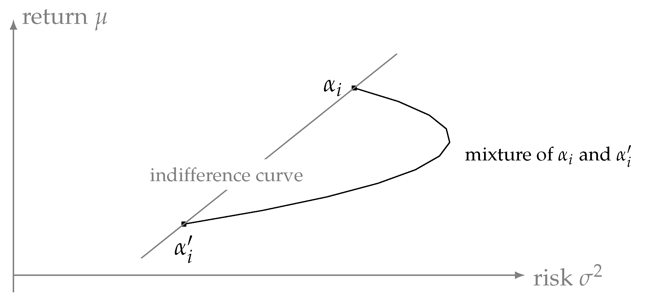
We now consider a game where a player chooses a possibly mixed strategy given the possibly mixed strategy profile of other player(s); then the player faces a lottery where material payoffs depend on the specified game, and probabilities depend on the strategy profile. For a given strategy of the other player(s), each strategy of a player represents a point in the – diagram given the expected value and the implied variance of the strategy; i.e., for any strategy this point is determined by and . We will show that mixing between two strategies of player i with the same utility (see Figure 1, where these strategies are denoted and ) actually leads to a of utility as the variance increases. This is in sharp contrast to the usual “egg shaped” efficient frontier seen in almost every textbook in finance, where mixing decreases the variance and therefore contributes to an increase in utility.
One main difference relative to other applications of non-generalized or generalized expected utility functions to game theory (see, for example, [25]) is that terminal node utilities of players are now dependent on how this terminal node is reached. In the case of random events, whether due to moves by nature or mixed strategies of one of the players, payoffs that are identical with respect to their material (or monetary) payoffs give rise to differences in utility under the – paradigm. That terminal node utility may depend on endogenous aspects of other players’ behavior has recently received some detailed attention under the heading of psychological game theory (see, for example, [15,16,26]) where beliefs of players matter for the utility payoffs of players). – utility in games implies that strategies and the history of play, whenever random events are involved, affect the utility.
We proceed by first defining games based on – utility functions and study static 2 × 2 and N × N games based on linear utility functions. We then discuss nonlinear – utility functions.
2. Definition of Static – Games
To understand the applicability of – utility functions to games, we start by analyzing static games with complete information. We consider games with a finite set N of players and nonempty and finite sets () of actions. Any profile of pure strategies will provide player i with a material (not utility) payoff ; we use the notation .
We consider mixed strategies—that is, elements of . Let be a profile of mixed strategies, that is, a vector with . Furthermore, with is the probability that player i will play the pure strategy and for .
Player i can expect the following material payoff from strategy combination
and a variance of
For ease of notation we use and Var
Definition 1.
A μ–σ game is a game where the utility of player from strategy combination α is given by a μ–σ utility function
is strictly increasing in the first variable and strictly decreasing in the second variable, and is strictly quasiconcave in μ and.
We assume strict quasiconcavity to ensure uniqueness of the solution to classical maximization problems in finance. Relaxing this assumption most likely does not alter our results but makes the arguments very tedious.6
We first analyze the case of two players. Furthermore, we assume that the utility function is of the following simple linear form:
with r being the parameter for the strength of the variance aversion.7 We refer to a utility function of this form as linear utility.8
In the next paragraphs we analyze the effect of this utility model in well known examples of the literature on game theory. This allows us to show that in – games a Nash equilibrium does not always exist.
3. First Results for – Games
3.1. Best Response with Linear Utility
Compared to standard game theory, – games may have different sets of equilibria. In standard game theory mixed strategies, i.e., strategies that randomize over actions that lead to the same expected (material) utility, yield the same utility payoff for a player, due to the the linearity in probabilities assumed by the expected utility framework. For – games the randomization of a mixed strategy comes at a price.
Given the behavior of the other player(s) in the game, the following maximization problem determines the best response of a player with – utility.
This is a quadratic equation in , where the coefficient on the quadratic term is always negative.
Lemma 1
(best response with mixed strategy). In equilibrium a player with μ–σ utility does not choose a mixed strategy, unless all actions chosen with positive probability are characterized by the same expected value and the same variance—i.e., they are characterized by the same point in the μ– diagram.
Proof.
We show first that all convex combinations of two (mixed) strategies lie on a convex curve in a – diagram. Let and be two strategies of player i. Expected value and variance given the strategies of other players can be denoted as
Let a convex mixture choose times to play and times to play ; we refer to this strategy as . The expected value can then be calculated following (1):
and the variance is given as
In the case that
and the second derivative is given as
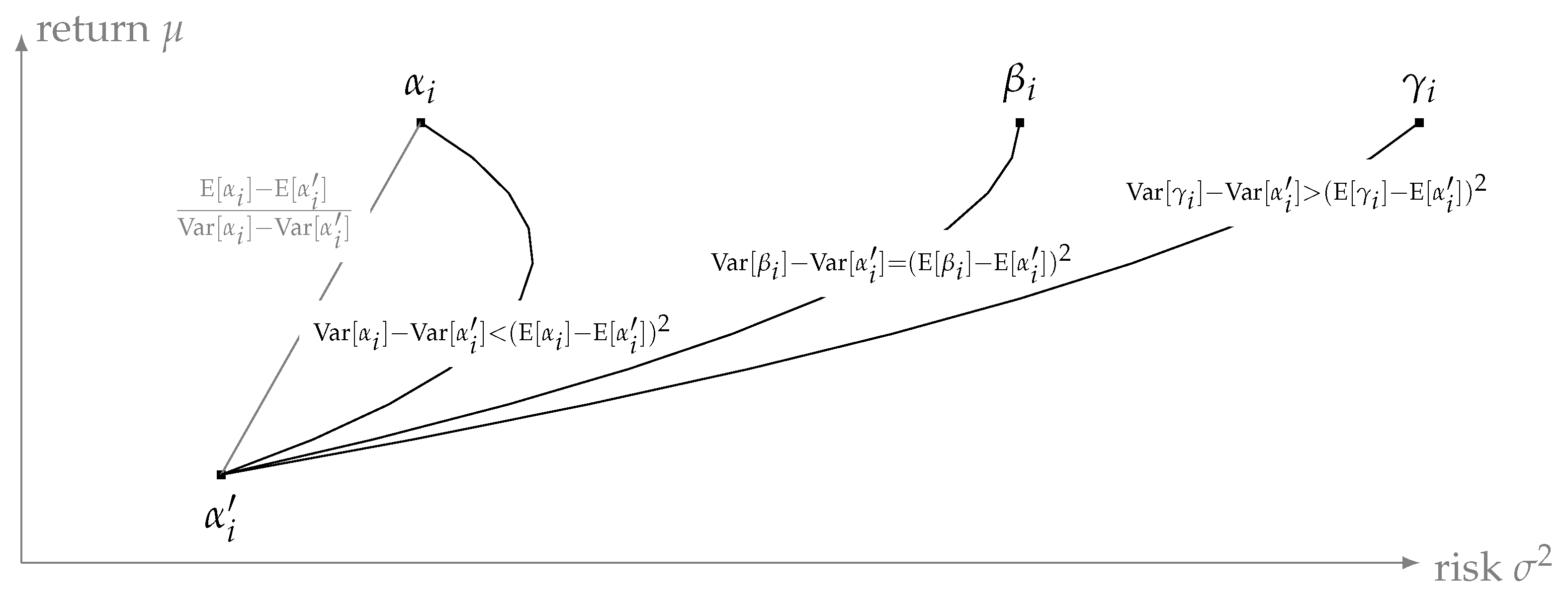
Therefore, any convex combinations of two strategies lie on a convex curve. Figure 2 illustrates such curves for three different combinations of strategies.
Our result follows from the observation that indifference curves of a player in the – diagram are given by straight lines between two strategies, given the linear utility function . For this reason any convex combination of strategies must be worse than either of the strategies that are combined. Even if a player is indifferent between two strategies and , he will see any mixture between these strategies as inferior. □
This implies an equilibrium in mixed strategies only exists if both strategies are represented by the same point in the – diagram—i.e., they do not only have the same expected material payoff but also lead to the same variance.
Although this lemma seems to be related to Lemma 1 in [14], our model differs from theirs in one substantial point. The set of all pure actions in [14] is convex, which is not the case in static games with a finite number of pure strategies. Similarly, [13] looked at games where the players violate von Neuman and Morgenstern’s independence axiom, and assumed that the preferences (in terms of payments) were quasiconcave. Again, our paper differs from that work because (in terms of payments) – utility functions need not be quasiconcave.9
We next study the implication of this with respect to the best response towards a pure strategy and when an equilibrium in mixed strategies exist.
Lemma 2
(best response given pure strategies of another player). The best response to a pure strategy is a pure strategy, unless the material payoff of the player under consideration is the same for a set of at least two actions. Any (best response) mixed strategy can only randomize over this set of actions.
Proof.
Referring again to Figure 2. Given that the other player chooses a pure strategy, all strategies of the player under consideration will be a point on the -axis. This implies that the point higher on the axis will be chosen unless two strategies lead to exactly the same material payoff. □
3.2. 2 × 2 Games with Linear Utility
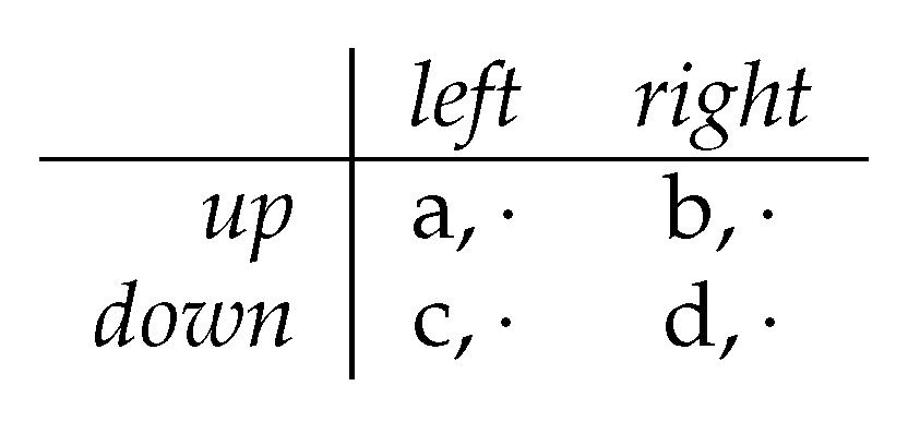
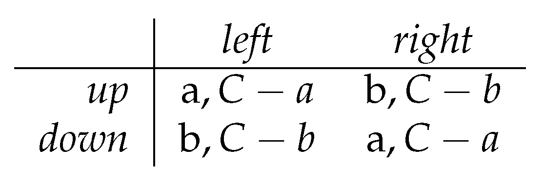
To answer the question when mixed strategy equilibria exist in – games, we start with the case of 2 × 2 games. The game we consider is given in Figure 3. We state our result for player 1 (the row player) and denote by q the probability that player 2 (the column player) chooses left. The following lemma characterizes the necessary condition for a best mixed strategy best response in comparison to the condition assuming standard expected utility theory.
Lemma 3
(best response in 2 × 2 games). The best response in any 2 × 2 game is a mixed strategy if and only if, (a) the usual condition of expected utility game theory holds,
and (b) the following condition is true:
This lemma shows that 2 × 2 – games do not have more mixed equilibria than an equivalent standard 2 × 2 game. Being a mixed strategy equilibrium in the standard game is a necessary but not sufficient condition for being an equilibrium in the equivalent – game. The second condition (6) has to be fulfilled as well; therefore, many – games will not have any equilibrium.
Condition (6) has an insightful interpretation. It requires that, given any pure strategy of the other player, the sum over all material payoffs that the player is able to achieve over all his strategies is constant, i.e., independent of the pure strategy that is chosen given the randomization of the other player. Regardless the other player’s choice, it is only the slice of the cake and not the size of the cake that is determined by the player’s own actions.
Proof.
We apply Lemma 1, which implies for the 2 × 2 game that expected value and variance have to be the same for any variation in the probability p of player 1 to choose up. This leads to the following two conditions:
The constant expected value implies
A non-degenerate mixed equilibrium requires , and thus and . Simplifying the condition under constant variance by solving for and calculating the first-order condition p, gives us the second condition, so it follows as
Combining both conditions gives us the second condition for the existence of a mixed equilibrium . □
We next characterize the games where mixed equilibria do survive.
Theorem 1
(Mixed Equilibria in 2 × 2 games). A mixed equilibrium in 2 × 2 μ–σ games with linear utility functions exists if and only if
- (i)
- The candidate for equilibrium is a mixed equilibrium of a standard (expected utility) game with utility payoffs equal to the monetary payoffs of the μ–σ game;
- (ii)
- For each strategy of the other player, the sum of monetary payoffs of a player is the same for the strategies available to the player.
Proof.
In the following we discuss special cases. We start by analyzing zero-sum games.
Theorem 2
(2 × 2 zero-sum games). The only 2 × 2-μ–σ zero-sum game with an equilibrium in non-degenerate mixed strategies is matching pennies.
Proof.
We denote the material payoffs as given by Figure 4.
Given the previous results, we know that the following two conditions have to be fulfilled in a mixed strategy equilibrium
Given that we study zero-sum games we know
Substituting the last equation into the previous two, gives us
Adding this equation to (8), yields and and and ; therefore, Figure 5 represents this game. □
Our next result concerns non-zero-sum games. It is well-known—despite disturbing results in – theory—that a portfolio with higher payoffs is not necessarily preferred by an investor (preferences need not be monotone).10 Therefore, it is not clear that dominated strategies in – games cannot be equilibrium strategies. In 2 × 2 games we can show the following result.
Theorem 3
(2 × 2 games with dominated strategies). If a strategy in a 2 × 2 game is dominated in monetary payoffs, then no mixed equilibrium of the 2 × 2 μ–σ games exists.
Proof.
This follows immediately from the fact any equilibrium of the – game must be an equilibrium in the equivalent expected utility framework. In expected utility, games dominated strategies never receive a positive probability weight. □
While this result seems to be obvious at first, it is less so if one considers that a player’s monetary payoff choosing the—in monetary payoffs—dominant action may lead to a higher variance than the dominated action over compensating for the loss in payoff. As the result shows, this cannot be the case. These results have a set of implications that are noteworthy:
- Only coordination games and games without a pure strategy equilibrium in the expected utility framework can have mixed strategy equilibria.This follows from the observation that solving (5) for q and substituting (6). Given , either one action dominates the other or players prefer payoffs in two diagonal corners. Theorem 3 rules out the former, leaving the cases where both players either prefer the same two diagonal corners (coordination games) or they prefer different corners—games without a pure strategy equilibrium in standard games.
- Battle of sexes – games do not have a mixed strategy equilibrium unless players—in case of miscoordination—receive an additional payoff equal to the difference in their payoffs between the preferred and the alternative equilibrium.
3.3. N×M Games with Linear Utility
Mixed equilibria in 2 × 2 – games only exist if an additional constraint on payoffs holds to ensure that these strategies are a best response. In this section we show that for N × M games a mixed equilibrium only exists if the game is degenerate. To show this, we show that any best response avoids mixing unless the material payoff for this player are constant over all possible outcomes of the game.
Theorem 4
(best response with N × M games). In an N × M μ–σ game () in any mixed equilibrium, players randomize at most over two pure strategies, unless the payoffs to the player are constant (independent of his choice).
Proof.
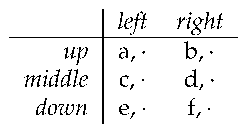
Again, we study the best responses of players. From Lemma 1 we know that any action that may be chosen by a player will have to be represented by the same point in the – diagram. To illustrate our argument, let us assume that a player randomizes over 3 actions, while the other player randomizes only over two. To show this, consider the 3 × 2 game with material payoffs given in Figure 7.
Let , and be the probabilities that the player chooses up, middle, and down respectively. The condition for a constant expected value in this case is
This is a condition on two variables, which gives us two constraints:
If one combines both, they imply also . Any nondegenerate mixed equilibrium implies that which immediately implies .
Furthermore the variance needs to be constant:
This is a condition on two variables, and using derivatives it can be reduced to two equations
and thus . Solving implies
These three equations imply that and , which contradicts the condition for the constant expected value. □
3.4. A Game with Nonlinear Utility Functions
The results of the former section heavily depend on the fact that we restricted ourselves to linear – utility functions. If we consider other utility functions it might well be that an equilibrium in mixed strategies exists, although the restrictive condition (6) is not met. In order to show this result, we consider the following utility function:
Its indifference curves are convex and monotone functions in the - diagram.
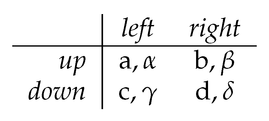
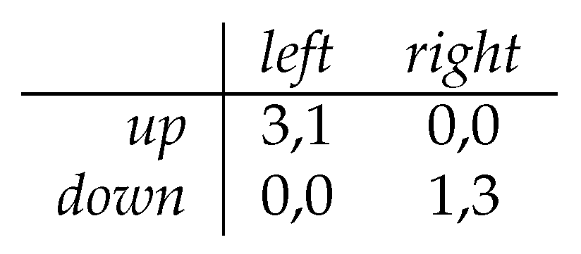
We now look at a game where the material payoffs are given by Figure 8. We can now show that is a mixed equilibrium of the game. Notice that in classical game theory (where utilities are given by Figure 8) an equilibrium would be given by .
Assume that the row player chooses . Then the utility of the column player is given by
This function has a maximum of in . Hence, the best response is a mixed strategy. With the same reasoning we can show that is the best response to the own player’s strategy .
4. Conclusions
We applied – utility to game theory. Using monetary games we discussed how equilibria predictions—in particular with respect to the existence of mixed equilibria in static games—change if behavior can be described by preferences depending on the mean and variance of random payoffs. This is an alternative to models of generalized expected utility which relax the assumption of linearity in probabilities, which is the basis of von Neuman and Morgenstern’s expected utility model. While generalized expected utility models still maintain the assumption that terminal utilities are independent of the way the respective endpoint is reached, – theory allows us to capture endogenous uncertainty caused by mixed strategies of players. In the case of the 2 × 2 games we were able to show that mixed strategy equilibria do survive in a – game under a set of additional restrictions. Thus, the set of mixed equilibria in a – game is a subset of the mixed equilibria of the equivalent game where the monetary payoffs are interpreted as utility payoffs.
Our analysis is based on the interpretation of mixed strategies as randomization by players over their actions, and not as the beliefs about actions of the other player or of the composition of a population of other players playing pure strategies from which the other player is randomly drawn.11 In this case mixed equilibria only survive in – games if there is a substantial gain from randomizing, for example, because allowing the other player to predict one’s behavior comes at a first order cost effect, as in the case of zero sum games.
We believe this analysis can help to capture the experimentally observed aversion against mixing by players. While the – model is a very specific abstraction and somewhat arbitrary, its prominence in finance and its capability to capture uncertainty endogenous to the play of the game, made it for us a worthwhile starting point to reconsider equilibria when one departs from using utility function that can be characterized by Choquet integrals.
Author Contributions
Methodology, writing, and formal analysis: Both authors contributed equally. All authors have read and agreed to the published version of the manuscript.
Funding
This research received no external funding.
Conflicts of Interest
The authors declare no conflict of interest.
References
- Von Neumann, J.; Morgenstern, O. Theory of Games and Economic Behavior; Princeton University Press: Princeton, NJ, USA, 1947. [Google Scholar]
- Allais, M. Le Comportement de l’Homme Rationnel devant le Risque. Econometrica 1953, 21, 503–546. [Google Scholar] [CrossRef]
- Ellsberg, D. Risk, Ambiguity, and the Savage Axioms. Q. J. Econ. 1963, 75, 643–669. [Google Scholar] [CrossRef] [Green Version]
- Quiggin, J. A Theory of Anticipated Utility. J. Econ. Behav. Organ. 1982, 3, 225–243. [Google Scholar] [CrossRef]
- Yaari, M.E. The Dual Theory of Choice under Risk. Econometrica 1987, 55, 95–115. [Google Scholar]
- Segal, U. The Ellsberg Paradox and Risk Aversion: An Anticipated utility Approach. Int. Econ. Rev. 1987, 28, 175–202. [Google Scholar]
- Cochrane, J.H. Asset Pricing, 2nd ed.; Princeton University Press: Princeton, NJ, USA, 2005. [Google Scholar]
- Fama, G.; French, K. The cross section of expected returns. J. Financ. 1992, 47, 427–465. [Google Scholar] [CrossRef]
- Markowitz, H.M. Portfolio Selection. J. Financ. 1952, 7, 77–91. [Google Scholar]
- Lajeri-Chaherli, F.; Nielsen, L.-T. Parametric characterizations of risk aversion and prudence. Econ. Theory 2000, 15, 469–476. [Google Scholar]
- Lajeri-Chaherli, F. More on Properness: The Case of Mean-Variance Preferences. Geneva Risk Insur. Rev. 2002, 27, 49–60. [Google Scholar]
- Meyer, J. Two Moment Decision Models and Expected Utility Maximization. Am. Econ. Rev. 1987, 77, 421–430. [Google Scholar]
- Crawford, V.P. Equilibrium without Independence. J. Econ. Theory 1990, 50, 127–154. [Google Scholar] [CrossRef] [Green Version]
- Chen, H.-C.; Neilson, W.W. Pure-strategy equilibria with non-expected utility players. Theory Decis. 1999, 46, 19–209. [Google Scholar] [CrossRef]
- Rabin, M. Incorporating Fairness Into Game Theory and Economics. Am. Econ. Rev. 1993, 83, 1281–1302. [Google Scholar]
- Battigalli, P.; Dufwenberg, M. Dynamic Psychological Games. J. Econ. Theory 2009, 144, 1–35. [Google Scholar] [CrossRef]
- Choquet, G. Theory of capacities. Ann. l’Inst. Fourier 1953, 5, 131–295. [Google Scholar] [CrossRef] [Green Version]
- Löffler, A. Variance aversion implies μ-σ-criterion. J. Econ. Theory 1996, 69, 532–539. [Google Scholar] [CrossRef]
- Battigalli, P.; Samuelson, L.; Van Huyck, J. Optimization Incentives and Coordination Failure in Laboratory Stag Hunt Games. Econometrica 2001, 69, 749–764. [Google Scholar]
- Al-Ubaydli, O.; Jones, G.; Weel, J. Patience, cognitive skill, and coordination in the repeated stag hunt. J. Neurosci. Psychol. Econ. 2013, 6, 71–96. [Google Scholar] [CrossRef] [Green Version]
- Agranov, M.; Healy, P.J.; Nielsen, K. “Non-Random Randomization”, Working Paper. 2020. Available online: https://ssrn.com/abstract=3544929 (accessed on 11 January 2021).
- Raiffa, H. Risk, Ambiguity, and the Savage Axioms: Comment. Q. J. Econ. 1961, 75, 690–694. [Google Scholar] [CrossRef]
- Eichberger, J.; Kelsey, D. Uncertainty Aversion and Preference for Randomization. J. Econ. Theory 1996, 71, 31–43. [Google Scholar] [CrossRef] [Green Version]
- Harsanyi, J.C.; Selten, R. A General Theory of Equilibrium Selection in Games; MIT Press: Cambridge, MA, USA, 1988. [Google Scholar]
- Dekel, E.; Safra, Z.; Segal, U. Existence and dynamic consistency of Nash equilibrium with non-expected utility preferences. J. Econ. Theory 1991, 55, 229–246. [Google Scholar] [CrossRef]
- Geanakoplos, J.; Pearce, D.; Stacchetti, E. Psychological Games and Sequential Rationality. Games Econ. Behav. 1989, 1, 60–79. [Google Scholar] [CrossRef] [Green Version]
- Nielsen, L.T. Portfolio selection in the mean-variance model: A note. J. Financ. 1987, 42, 1371–1376. [Google Scholar] [CrossRef]
| 1. | |
| 2. | |
| 3. | See [17]. |
| 4. | See [18] for an axiomatic foundation of – utility functions based on preference axioms. That – utility functions are not a special case of a Choquet integral using some capacity can easily be seen: Choquet integrals are homogenous of degree one, a feature that many – functions (for example, –) do not possess. |
| 5. | However, notice that [21] found very high rates of randomization in their experiments. |
| 6. | See the discussion in [10]. |
| 7. | |
| 8. | Note, this utility function shares with CARA expected utility functions the characteristic that the preference overall risk is independent of the wealth or income level. |
| 9. | Using suitable numbers, one can already show that has upper contour sets that are not convex. |
| 10. | This particular feature of – preferences is well known; see, for example, [27]. The fact that the CAPM as an application of – is still used today shows that the non-monotonicity is not regarded as a major problem in finance. |
| 11. | With the population interpretation, selection criteria, particularly payoff dominance ([24]), become important. Payoff dominance does not select mixed equilibria in coordination games, as these minimize the expected payoff, and it is difficult to argue why a population’s composition should yield this result. – theory applied to game theory gives us in the case of coordination games a similar prediction. |
Figure 1.
Mixing two lotteries and with the same utility decreases the utility in a – game.

Figure 2.
Mixtures of three pairs of strategies , and in the - diagram.

Figure 3.
Material payoffs for best response function.

Figure 4.
Material payoffs in the game of Theorem 2.

Figure 5.
Matching pennies—the only – zero-sum game with (non-degenerate) mixed strategies.

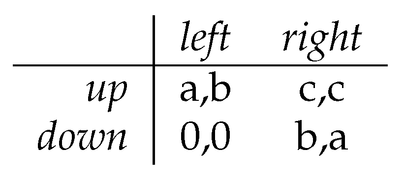
Figure 6.
Battle of sexes with mixed strategy equilibrium ().

Figure 7.
Material payoffs for best response function in a 3 × 2 game in the proof of Theorem 4.

Figure 8.
Material payoffs of a game with nonlinear utility.

Publisher’s Note: MDPI stays neutral with regard to jurisdictional claims in published maps and institutional affiliations. |
© 2021 by the authors. Licensee MDPI, Basel, Switzerland. This article is an open access article distributed under the terms and conditions of the Creative Commons Attribution (CC BY) license (http://creativecommons.org/licenses/by/4.0/).
Share and Cite
MDPI and ACS Style
Dulleck, U.; Löffler, A. μ–σ Games. Games 2021, 12, 5. https://0-doi-org.brum.beds.ac.uk/10.3390/g12010005
AMA Style
Dulleck U, Löffler A. μ–σ Games. Games. 2021; 12(1):5. https://0-doi-org.brum.beds.ac.uk/10.3390/g12010005
Chicago/Turabian StyleDulleck, Uwe, and Andreas Löffler. 2021. "μ–σ Games" Games 12, no. 1: 5. https://0-doi-org.brum.beds.ac.uk/10.3390/g12010005
Note that from the first issue of 2016, this journal uses article numbers instead of page numbers. See further details here.