
Trust and Trustworthiness in Corrupted Economic Environments


1
Department of Economics, Law and Institutions, University of Rome Tor Vergata, Via Columbia, 2, 00133 Rome, Italy
2
Centre for Financial and Management Studies, SOAS University of London, London, 10 Thornhaugh St, Bloomsbury, London WC1H 0XG, UK
3
Department of Economics and VERA, University of Venice “Ca’ Foscari”, Cannaregio, 821, 30121 Venice, Italy
4
Centre for North South Economic Research, Department of Economics and Business, University of Cagliari, V. le S. Ignazio, 17, 09123 Cagliari, Italy
*
Author to whom correspondence should be addressed.
Games 2021, 12(1), 16; https://0-doi-org.brum.beds.ac.uk/10.3390/g12010016
Submission received: 14 January 2021
/
Revised: 26 January 2021
/
Accepted: 29 January 2021
/
Published: 4 February 2021
(This article belongs to the Special Issue Laboratory Experiments: Cooperation, Sanctions and Norms)
Abstract
:We use an original variant of the standard trust game to study the effects of corruption on trust and trustworthiness. In this game, both the trustor and the trustee know that part of the surplus they can generate may be captured by a third “corrupted” player under different expected costs of audit and prosecution. We find a slightly higher trustor’s giving in the presence of corruption, matched by a significant excess of reciprocity from the trustee. Both the trustor and the trustee expect, on average, corruption to act as a tax, inelastic to changes in the probability of corruption prosecution. Expectations are correct for the inelasticity assumption and for the actual value of the “corruption tax”. Our experimental findings lead to the rejection of four standard hypotheses based on purely self-regarding preferences. We discuss how the apparently paradoxical excess reciprocity effect is consistent with the cultural role of heroes in history, where examples of commendable giving have been used to stimulate emulation of ordinary people. Our results suggest that the excess reciprocity component of the trustee makes the trustor’s excess giving a rational and effective strategy.
1. Introduction
Trust is without a doubt among the most important and investigated characteristics and drivers of economic development.1 At the micro-level, most of the empirical experimental research in the field has been conducted using the well-known trust investment game [6]. In this sequential game, a first player (the trustor) can send part of her/his endowment to a second player (the trustee). The amount sent is tripled by the experimenter, and the trustee can decide to send back part (or all) of it to the trustee. The game reproduces some of the most important characteristics of human interactions in economic environments. Under imperfect information and incomplete contracts, individuals cooperate (and create extra value from cooperation) only if levels of trust and trustworthiness are high enough. Social capital under these two specific microeconomic dimensions is, therefore, at the root of creation of economic value.
A main characteristic of the standard trust investment game is that the two players (trustor and trustee) make their decisions by knowing that the surplus generated by the trustor will be entirely shared between them in their final game payoffs. Many social and economic environments in the world are, however, unfortunately plagued by crime and corruption.2 Studying trust and trustworthiness in difficult economic environments where agents know and expect that part of the generated payoffs may be reduced by the choices and actions of third agents is, therefore, of foremost importance. We make an original contribution to this literature by devising a variant of the standard investment game [13], where the trustor and the trustee know that part of the surplus that can be generated in the game can be extorted by a third-party subject to different expected audit probabilities. In this way, the game reproduces three typical characteristics of corruption, where the corruptor has monopoly power and discretion over a surplus, while knowing that a higher level of information will increase the probability of prosecution and penalty. The literature on trust and corruption has postulated a strong and negative correlation between the two variables. Evidence on the direction of the causal link between corruption and trust is, however, mixed, at best. On the one hand, some have taken the view that low levels of trust in a society may favor corruption because of the widespread sense of opportunism [14,15,16,17]) while others have shown that a lack of trust may generate a perception of high levels of corruption [18] that, in turn, renders corruption both more acceptable and more likely to occur [19,20]. On the other hand, many authors view corruption as one of the driving forces behind the erosion of trust [21,22,23]. Some have also discussed the possibility of a circular causality [24]: corrupt officials and business people tend to illegally appropriate an undue share of resources, thereby making the rich even richer. In this way, corruption fuels inequality, which leads to lower trust and even more corruption.
Endogeneity and the two-way causality links described above provide evidence that testing the trust–corruption causality with econometric studies on aggregate data is a difficult task. Randomized lab experiments can, therefore, be a valid alternative.
The only experiment, to our knowledge, that addresses the issue is [25]. In his design, participants first play either a harassment bribery game or a strategically equivalent ultimatum game. These games mimic a situation where extortion is an option. In the second stage of the experiment, with the aim of measuring the effect of the previous experience on trust, players interact in a standard trust game. Findings from this experiment show a negative spillover effect of corruption on trust.
Our approach is original, vis-à-vis the relevant work of [25], in several respects. First, we look at the impact of corruption on trust and trustworthiness within the same treatment. More specifically, the stylized corruption activity has a direct effect on players’ payoffs and does not enter the game as a spillover effect produced by the results and characteristics of a previous and independent treatment. In this respect, our treatment has an important element of external consistency, since corruption is modelled as extorting a share of the expected payoff of the trustor and the trustee and, as such, directly affecting their decisions of trust and reciprocity. Second, the above-described approach allows us to directly measure the expected perceived corruption and to analyze how it affects trustors’ and trustees’ choices. Third, with our design, we can evaluate the impact of different policies and, specifically, the relative deterrent effect of a high versus low probability of audit and a fine on both the actual third player behavior and the beliefs about corruption of the other two trust game agents. Fourth, with such a design, we can look at the impact of our treatments on a wide range of variables, such as trust, the conditional distribution of trustworthiness (elicited with the strategy method), the trustor’s first order beliefs, and strategic altruism (by measuring the trustor’s expected return on giving based on the expected reply of the trustee and the behavior of the third player).
The well-known trade-off between lab experiments and standard econometric analysis passes through the external consistency and capacity of isolating causal relationships. We accurately design our experiment to limit problems related to the first point. First and foremost, the experimental design properly reproduces the consequence of corruption under the form of bribery (i.e., a “tax” on the monetary payoffs of economic agents), subject to a risk of audit and penalty. Second, in the experiment, the third-party agent only chooses how much to subtract of the surplus generated during the interaction between the trustor and the trustee. This consideration has two main consequences that allow us to interpret the strategic interaction in terms of corruption. On the one hand, there is no possibility for the third-party agent to improve social welfare. On the other hand, the choice domain of the third-party agent is confined within the outcome of the trust game, thus excluding the possibility to impact (as, for instance, in settings with agents who can steal/destroy others’ initial endowment) the strategy set of both the trustor and trustee. Third, in our design, we use a real effort game to assign roles, relegating the third-party agent to the worst performing subject. This is done to foster the perception (beyond the information on the probability of audit and the penalty given by the experimenter) that the third player is withdrawing part of the other two players’ payoffs without being entitled to it [26]. Fourth, the audit procedure used in the experiment to detect and fine the third-party agent qualifies the negative connotation of corruption in that it gives the idea to all subjects that what the third player does is close to bribery (and not just to legal taxation). Even though we are clearly aware that external consistency in a lab cannot be perfect, we believe that, for the reasons explained above, the design can reasonably capture some of the main elements involved in a fiduciary relationship in the presence of risk of extortion.
Testable Predictions and Summary of Findings
We use our experiment to test four null hypotheses on the three players’ behavior under the standard assumption of purely self-regarding preferences being common knowledge. Under this theoretical benchmark, we expect (i) the trustor’s giving to be zero (with the exception of the special case, where, for strategic reasons, she expects that the trustee and the third agent are not purely self-regarding and that trust pays), (ii) the trustee’s giving to be zero, and (iii) the third player’s withdrawal to be equal to 100 percent of the game surplus.
With reference to our theoretical benchmark, a first important finding is that all the formulated null hypotheses are rejected. Trustees and trustors (even when they expect that trust does not pay) give more than zero, and the third agent’s withdrawal rate is significantly less than 100 percent (and is expected to be so by trustors and trustees). A second important result is that trustees’ choices are positively and significantly related to the level of trustor’s giving and are, therefore, consistent with the alternative theoretical benchmark of reciprocity. A third important general finding is the slightly higher (and not lower) level of trust in treatments with corruption, matched by a significant effect of excess reciprocity from the trustee. We comment on this last finding by considering its consistency with an alternative view of human preferences where commendable giving triggers excess reciprocity, thereby justifying the role of and emphasis on heroes in all cultures and traditions.
The rest of the paper is organized as follows. In the second section, we present the experimental design. In the third section, our empirical findings are separately examined for trustors, trustees, and third corrupting agents. In the fourth section, we conclude and resume the main findings and their implications for the literature.
2. The Experimental Design
2.1. Baseline Game and Additional Treatments
The baseline treatment, TC (trust + corruption), consists of a sequential game involving three players: A, B, and C (Figure 1).
Let , , and denote the choices of the three players, respectively. At the beginning of the game, all three players are endowed with an initial, exogenous endowment, . In the first two stages of the game, A and B participate in a standard trust game. Specifically, in the first stage, A chooses how much of the endowment to send to B, with . Whatever A sends to B is multiplied by a coefficient , so that the amount effectively received by B at the end of the first stage is . In the second stage, B chooses how much of that amount to return to A, with . Thus, at the end of the second stage, the (temporary) payoffs of A and B from the trust game are given by , for A, and , for B.
Notice that, regardless of the choice made by B, the sum of A’s and B’s payoffs from the trust game is , thus being uniquely determined by the size of the exogenous, initial endowment, , and the choice of A. Let denote the “surplus” generated in the trust game, namely, the increase in the overall amount of resources at stake in the interaction. By the previous considerations, is a function of the choice of the trustor, A.
In the third stage of the game, the corruptor, C, chooses how much of the surplus to keep for herself, with . Whatever C decides to keep reduces A’s and B’s payoffs from the trust game in proportion to the share of surplus, , acquired by the subject in the trust game. More specifically, given , the reductions in payoffs imputed to A and B are expressed by and , respectively, where , , and .
C’s choice completes the sequential game, and the final payoffs are , , and , for A, B, and C, respectively.
We compared results from the baseline game TC with a modified version introducing the possibility for C of withdrawing part of the surplus produced by the other two players at the end of the game.
In the base treatment, TNC (Trust + No Corruption) the third agent, C, cannot make any choice and simply receives feedbacks about the size of the surplus generated in the trust game. Thus, in TNC, the final payoffs of the three players are given by , , and for A, B, and C, respectively.
In the corruption treatment, we studied the effects exerted by the opportunity given to the third player, C, of withdrawing part of the surplus generated by the other two players (with different audit probabilities). In particular, before making their choices in the TC_p (Trust + Corruption + Audit with probability p) treatment, all subjects are informed that, at the end of the game, C’s choice will be audited with positive probability . More specifically, we have three different versions of the corruption treatment, with p set at 0, 10 percent, and 50 percent, respectively. The audit procedure influences C’s final earnings only, while the expressions of A’s and B’s payoffs remain unchanged with respect to those in TC. In particular, if audited and found to have kept a positive amount of the surplus , the payoff of the corruptor, C, is reduced by plus a sanction that is proportional to the size of . Specifically, the expected final payoff of C in TC_p is given by , where represents the flat fine rate that the corruptor pays on , if audited.
2.2. Procedures
Upon their arrival in the laboratory, subjects were randomly assigned to a computer terminal. At the beginning of the experiment, subjects were randomly and anonymously assigned to groups of three and were given a general description of the sequential game. In particular, subjects in TC_p were told that the interaction involved the following three phases (Figure 2).
Phase 1: the “slider task” competition. In the first phase, the three roles, A, B, and C, were assigned to group members depending on subjects’ relative performance in the “slider task” real effort game [27]. The task consists of a single screen displaying a number of “sliders”, and the layout of the screen was kept unchanged across subjects and sessions. All of the sliders on the screen were initially positioned at the left margin, which corresponds to the value of 0. By using the mouse, the subject could change, an unlimited number of times, the position of each slider at any integer location between 0 and 100 inclusive. She was awarded a point whenever she managed to position a slider to the value of 50. At the end of the slider task, the score obtained by each subject was given by the number of sliders she centered to the value of 50 within an allotted time of 120 s. As the task proceeded, the screen displayed the subject’s current points score and the amount of time remaining. At the end of the first phase, subjects were only informed about their final score and whether it ended up in the two best performances of the group. The two best performers in the group were randomly assigned to either role A or role B, while the subject with the lowest score was assigned to role C. Ties were broken randomly.
It is worth noting that our mechanism does not exclude the possibility that a player C in one group obtains a score that is higher than those of players A and B in a lower performing group. However, the average score of player C is significantly lower (9.7; 95% confidence interval: [8.19; 11.20])) than those of players A (20.05; 95% confidence interval: [17.97–22.12]) and B (mean score: 19.93; 95% confidence interval: [17.90–21.96]).
It might be argued that assigning roles on the basis of performances in a slider task might cause selection into roles. However, both the simplicity of the task and the fact that the subjects were not required to properly demonstrate any specific skills (field of study, professional profile, etc.) reduces the extent of the potential bias from selection (our point is confirmed by empirical evidence on balancing properties discussed in Section 3). On the contrary, two considerations justify this procedure. First, competing in the slider task could introduce a sense of entitlement to participate in the trust game, rather than being relegated to the mere role of C, who either made no choice in the experiment (in TNC) or could only subtract resources from A and B (in TC and TC_p). Indeed, in line with [28], we believe that effort and work performance—more than luck, birth, and wealth—better capture what an individual “deserves”. Moreover, there are studies assigning property rights [29] and roles in groups [30] based on subjects’ performance in the slider task. Second, by making the difference between best and worst performers salient, the slider task enhanced the existing conflict of interest between the trust game participants, A and B, and the corruptor, C.
Phase 2: the trust game. At the beginning of the second phase, each of the three subjects of the group was assigned to an exogenous endowment of ten tokens, namely, . Then, A and B participated in the trust game with the efficiency parameter set to . The strategy method was used to elicit B choices. In particular, before being informed about A’s decision, B chose how much to return to A for each possible choice that A could have made. B knew that, of all her 10 choices (one for each of the admissible values of in ), only the choice corresponding to the amount effectively sent by A would be used to determine payoffs. The decision to use the strategy method for eliciting B’s choice allows us to collect detailed information about B’s conditional behavior and to assess whether her attitude to reciprocate is affected by the presence of the corruptor and the existence of formal rules of auditing and prosecution.
Phase 3: the choice of C and the audit procedure. The choice of C is also measured with the strategy method. Namely, the player chose how much of the surplus to keep for any possible choice of A. Again, C knew that, of all her 10 choices (one for each of the admissible values of in , only that corresponding to the amount effectively sent by A would be used to determine payoffs. The audit procedure was administered by the PC. In particular, subject C was told that the computer would have randomly selected one of 100 tickets, numbered from 1 to 100. If the number of the ticket was smaller than p, then the choice of C was audited. We used two values of p, either 10 or 50, thus generating two treatments: TC_50, in which the probability of auditing was fifty percent, and TC_10, in which the probability was ten percent. In both treatments, we set the penalty rate , implying that, in the case of auditing, C was convicted to pay a fine of one token for every two subtracted from the surplus, . The value of was chosen to avoid bankruptcy of C.
All the relevant rules for determining payoffs, in addition to information about how C’s choice affected A’s and B’s payoffs, were provided at the beginning of the experiment and included in the general description of the game. Specific instructions for each of the three phases were distributed at the beginning of each phase and read aloud. Before starting with each phase, subjects answered several control questions to confirm their understanding of the experimental rules and, when necessary, they were assisted by researchers to ensure their full understanding of the rules.
In designing our experiment, we had to choose whether to use an absolutely neutral language to write the instructions or frame them in a strong way for the “corruption” element of our treatment. We opted for an intermediate solution by not quoting explicitly the word “corruption” but letting players know in the instructions that the third player C would be audited with a given probability in some treatments and fined if caught taking part in the surplus. The reason for this intermediate choice was to avoid confusion with redistribution games (where there is no penalty when part of the value generated is given to another player) or, on the opposite, to avoid experimenter’s demand effect in presence of too explicit framing. Finally, we elicited belief measures about B’s and C’s choices by using an incentive compatible mechanism. To minimize the risk of hedging between choices and beliefs, subjects were informed about the belief elicitation procedure after phase 3 and before receiving feedback on subjects’ choices and payoffs. Again, instructions were distributed and read aloud. Measurement of beliefs is important since the gap between beliefs and actual behavior of the counterpart allows us to test whether observed findings are consistent with some specific preference structures (i.e., as it is well known that strategic giving occurs when trustor giving is inferior to the amount she/he expects to receive by the trustee). In our game, we measure the trustor’s and trustee’s beliefs about the behavior of the third agent (which corresponds to the corruption tax) since both beliefs are needed to understand whether trustor giving is strategic or not.
A’s first order and B’s second order beliefs in the trust game. We collected A’s guesses as to the amount returned by B and B’s guesses as to the amount A expected her to return in the trust game. Since B made her choice in strategy method, A and B were asked to state beliefs for each of the 10 potential choices that B could make. A and B were also told that, at the end of the experiment, one of the ten guesses would be randomly picked by the computer. In case the selected conjecture turned out to be correct, the participants received three tokens in addition to the payoff of the three phases.
A’s and B’s first order beliefs about C’s choice. We collected A’s and B’s guesses as to the share of surplus generated in the trust game that was kept by C in the third phase of the experiment. Again, since C made her choice of strategy method, A and B were asked to state beliefs for each of the 10 potential choices that C could make. As for before, at the end of the experiment, the computer randomly selected one conjecture, and A and B were paid 3 tokens according to its correctness.
The only difference between TC_p (p = 0) and TC_p (p > 0) concerned the fact that, in the former, we removed the audit procedure and, therefore, C did not face the risk of audit. Instead, the difference between TC_p and TNC was that, in the latter treatment, C did not make any choice and only observed the surplus generated in the trust game. In all treatments, the language used in the instructions was kept as neutral as possible and did not refer to sensitive words, such as “trust” and “corruption” (an English version of the experimental instructions used in TC_50 is included in Appendix A).
Subjects were informed that, during the experiment, payoffs and choices were expressed in tokens, rounded to the closest integer, if necessary. At the end of the session, the number of tokens accumulated during the experiment was converted at an exchange rate of EUR 1 for 2 tokens, and monetary earnings were paid in cash privately. On average, experiment participants earned about EUR 9.59 (including EUR 3 for showing up) for sessions lasting approximately 45 min, including the time for instructions and payments. Before leaving the laboratory, subjects completed a short questionnaire containing questions on their socio-demographics and their perception of the experimental task. We ran 3 sessions per treatment, each involving 15 subjects, for a total of 180 participants. The experiment took place in June 2017 in the Behavioral Economics Research Group (BERG) laboratory of the University of Cagliari. Participants were randomly recruited from the BERG subject pool, which consists of approximately 1000 students from a wide range of disciplines. The experiment was computerized using the Z-Tree software [31].
2.3. Hypothesis Testing
As is well known, with common knowledge on purely self-regarding preferences, the Nash equilibrium of a trust investment game is the “no investment”, “no return” situation, that is, the pair of strategies where the trustor gives 0 and the trustee cannot return anything but (and would in any case return) 0. The situation becomes different if the assumption of common knowledge of purely self-regarding preferences is relaxed. In such case, if the trustor believes that the trustee is other-regarding and that trust pays (i.e., the trustee will return more than what was initially sent), she may find it optimal to give a strictly positive amount of resources.
Conversely, the choice of a purely self-regarding trustee does not change conditional to the assumption of the counterpart’s (trustor’s) preferences. Her optimal conditional giving is null, even though she expects non-zero giving from the trustor.
Optimal strategies of the trustor and the trustee are also unaffected by the introduction of the third “corrupting” player in our modified trust investment game in three cases: the trustor’s giving with common knowledge of purely self-regarding preferences, and the trustee’s giving either with or without common knowledge of purely self-regarding preferences. In the fourth case, in which the trustor gives a positive amount of resources under the expectation of other-regarding preferences from the trustee, the choice depends on the effect of withdrawal of the third player (acting as a tax on the surplus created by the trustor in the game). There may be cases where the strategic altruism of the purely self-regarding trustor pays without the tax, but is expected not to pay with the tax since the gross trustors’ payoff (the trustors’ payoff net of tax) is expected to be higher (lower) when giving than when not giving. In these cases, the introduction of the third agent in the game modifies (reduces) the trustor’s giving.
Last, it is easy to observe that, in the case of purely self-regarding preferences, the third agent “levies” a 100 percent tax on the surplus produced by the other two players, in line with the expectation of zero giving from a purely self-regarding player in the dictator games.
These considerations led us to formulate the following three standard null hypotheses for our research:
Hypothesis 1 (H1).
When the trustor is purely self-interested, and such preferences are common knowledge, the possibility of withdrawal of part of the surplus from a third “corrupting” agent in the trust game has no effect on the trustor’s behavior. The trustor’s giving is zero both with and without corruption.
A variant of this hypothesis is that, when trustors believe that the trustee may give non-zero (purely self-regarding preferences are not common knowledge), but believe that trust does not pay, they will still choose zero giving based on their purely self-regarding preferences.
Hypothesis 2 (H2).
In a setting with purely self-regarding trustees, the possibility of withdrawal of part of the surplus from a third “corrupting” agent in a trust investment game has no effect on the trustee’s giving (with or without common knowledge of purely self-regarding preferences). The trustee’s conditional giving is zero, both with and without corruption.
Hypothesis 3 (H3).
In a setting with purely self-regarding trustors, where trustors expect that trustees are non-purely self-regarding, the possibility of withdrawal of part of the surplus from a third “corrupting” agent in a trust investment game has an effect on the trustor’s behavior (from zero to non-zero giving) if the trustor expects that his/her giving is expected to pay (not to pay) without (with) the tax (where for “pay”, we mean trigger a return that is higher than the amount sent).
Note that the previous hypothesis is based on the idea that trustors expect that trust pays in treatments without corruption, while it does not pay in treatments with corruption. To verify this conjecture, we need to calculate the trustor’s expected return from giving, as in Section 3.1.3.
Hypothesis 4 (H4).
If the third agent has purely self-regarding preferences, she will apply a 100 percent tax on the surplus created by the other two players in the corruption treatments without penalty.
The expected payoff for the third agent in the case of withdrawal is pwS(1 − p) − ( pwS/2)p, where pw is the share of the surplus withdrawn and p is the probability of being detected. The third agent, even if risk averse, will charge the highest (100 percent) tax in a corruption treatment without penalty (since she does not run any risk of being prosecuted) and in corruption treatments with penalty if she is not risk averse (since a higher tax will raise her expected payoffs). If she is risk averse and if her level of risk aversion is high, she may prefer less than 100 percent tax in treatments with a positive probability of audit since the decision to withdraw is equivalent to running a bet of increasing risk insofar as the withdrawal rate is higher.
3. Empirical Findings
We started our empirical analysis by testing whether balancing between corruption and non-corruption treatments is guaranteed (see Table 1).
We found a one-year difference between participants playing treatments with/without corruption (not significant at 95 percent), while the gender balance is almost the same (44 percent against 40 percent in corruption versus non-corruption treatments). The share of players doing voluntary activity is 44 percent against 51 percent in non-corruption versus corruption treatments, respectively (the difference is again not statistically significant). University years are, on average, three in both groups, even though students range from first year undergraduate to second year graduate. The share of those knowing game theory is approximately one third and is almost the same in both corruption and non-corruption treatments. In Table 2, columns 2 and 3, we report non-parametric tests showing that balancing properties are met within each role (trustor or trustee) between participants to corruption vs. non-corruption treatments. Moreover, we did not find significant differences in gender, age, self-assessed risk aversion, voluntary status, and share of players knowing game theory in two-by-two role comparisons (e.g., trustor versus trustee and trustor versus third corrupting agent). These findings confirm that selection into roles is not a problem in our experiment. To conclude, there are no relevant and significant differences in socio-demographic characteristics among players in corruption and non-corruption treatments and in two-by-two role comparisons. Consequently, we can conclude that balancing properties are met in our between design experimental setting.
3.1. Behavior of the Trustor
A first inspection of the behavior of our 60 trustors under the different treatments does not reveal any apparent significant effect of corruption on their behavior (Figure 3). From a descriptive point of view, trustors, surprisingly, give slightly more in corruption treatments and, specifically, 5.6 Experiment Currency Units (ECUs) in the treatment with zero probability of auditing of the third corrupting agent (TC_0), 4.53 ECUs in the treatment with 10 percent probability of auditing (TC_10), and 4.67 ECUs in the treatment with 50 percent probability of auditing (TC_50). The average trustor’s giving in the no corruption (TNC) treatment is 3.87 ECUs.
The difference between corruption and no-corruption treatments is, however, not significant under both parametric and non-parametric tests (two-sided Mann–Whitney rank-sum test, z 1.31, p-value 0.19). Note that this finding does not necessarily imply rejection of the hypothesis of the trustor’s purely self-regarding preferences under Ho(1), since evidence on the trustor’s giving per se is uninformative about the common knowledge assumption, that is, we do not know whether the trustor expects trust to pay (we verify this point in Section 3.1.1 and Section 3.1.2). In the first case, she can still have purely self-regarding preferences and opt for non-zero giving.
Upon deeper inspection of our data, also using information from our post-experiment questionnaire, we found that 40 trustors declare they have never studied game theory, while 20 declare that they have. If we look at the effect of game theory knowledge on the average trustor’s giving in games with corruption, we find that trustors who declare that they do not know game theory give significantly more (5.52 ECUs, against 3.33 ECUs from those who know game theory) (Figure 4). The non-parametric test on the difference in giving between the two groups of trustors created when using game theory knowledge as a discriminating factor rejects the null (z = 2.34, p-value 0.019 in the two-sided Mann–Whitney rank-sum test).
The problem here is that knowledge of game theory is not a randomized variable in our experiment. What we observed, therefore, may well be endogenous and due to a sorting and matching effect (i.e., individuals with stronger pro-social attitudes decide not to study game theory). This implies that, based on our evidence, we cannot prove that studying game theory reduces per se the trustor’s giving. Nonetheless, the observed significant correlation is of great interest, suggesting that heterogeneity in this specific population characteristic can produce relevant effects. In another part of our post-experimental questionnaire, we asked the players what strategy they followed (e.g., maximizing their own payoffs, maximizing payoffs of the team).
The share of individuals declaring that they acted to maximize their own payoffs was 50 percent among those who studied game theory and just 18 percent among those who did not study it. Meanwhile, the share of individuals declaring that they acted to maximize the team payoffs was 13 percent among those who studied game theory and 28 percent among those who did not study it. Therefore, we can associate knowledge of game theory with the prevalence of a purely self-regarding approach and ignorance of game theory with a different, more other-regarding (or we-thinking), attitude.
3.1.1. Behavior of the Trustor’s Expectations of the Withdrawal of the Third Agent
To check whether the different behavior of trustors, according to knowledge of game theory, was affected by either pure or strategic altruism, we parametrically investigated differences across treatments and determinants of trustors’ expectations of both the behavior of the third corrupting agent and the trustee’s strategy.
Specifically, the following table focuses on the trustor’s expectations about the behavior of the third corrupting agent.
Estimated findings show that average trustors’ expectations of a “corruption tax” (third player’s withdrawal rate) are approximately 62 percent, inelastic to differences in the probability of audit and a fine of the corruptor (see Table 2, column 1). However, if we introduce dummies for the expectation of trustors who know game theory, we find that these trustors expect a higher tax (almost 100 percent) in the treatment with corruption and zero probability of audit, while expecting a significantly lower tax in corruption games with probability of audit (see Table 2, column 2).
As we see in Section 3.3, the guess of trustors who know game theory is revealed to be too pessimistic, while that of trustors who do not know game theory is closer to the actual third agent’s withdrawal. This is because the third agent will “levy” a 70 percent tax (not significantly different from 62 percent, however, given the variability of forecasts, when using 95 percent confidence intervals), inelastic to the probability of audit. Fixed effects are, as expected, strongly significant, and their inclusion allows us to properly estimate the within effect of changes in the generated surplus on the expected third agent’s withdrawal.
3.1.2. Trustor’s Expectations of Trustee’s Giving
The next table parametrically analyzes differences across treatments and determinants of trustors’ expectations of the trustee’s giving.
On average, trustors predict a 1.23 payback ratio falling to around 1 in games with corruption and not the highest (50 percent) probability of audit (Table 3, column 1).
This means that trustors expect, on average, that trust will pay in terms of reciprocity (net of the intervention of the third corrupting agent) without corruption, or with corruption and high probability of audit.
Moreover, they expect that trust will not pay in games with corruption and zero or mild (10 percent) probability of audit. However, if we decompose the effect in separate estimates for trustors who either know or do not know game theory, we find that the payback ratio without corruption is much lower (around 1.06) for the former, falling substantially (by around 0.3) in games with corruption and not highest probability of audit (Table 3, column 2). In synthesis, trustors who know game theory expect trust to pay almost nothing in all treatments, while not to pay in those with corruption and mild probability of audit. Nonetheless, they choose non-zero giving in these last treatments, and these combined findings, therefore leading to the rejection of Ho(1), implying that the above-mentioned trustors cannot have purely self-regarding preferences.
Conversely, trustors who do not know game theory have higher expectations of trustees’ strategies, predicting an average payback ratio of 1.43 that falls by around 37 in games with corruption and not the highest probability of audit (Table 3, column 3). In synthesis, for these trustors, trust pays in terms of reciprocity (and weakly so, even in games with corruption and not the highest probability of audit). In Table 3, column 4, we simply re-estimate the model for the overall sample of trustors introducing slope dummies to check whether the observed differences between trustors who either know or do not know game theory are significant. Findings from this estimate show that the above-described differences in expectations between the two groups are significant.
3.1.3. Trustor’s Expectations of Returns of Her Strategies
To clarify the link between the trustor’s giving and her expectations of the trustee’s and third agent’s behavior (described in the previous two sections), we calculated the expected return on giving based on the above-mentioned two expectations (separately looking at agents either knowing or not knowing game theory).
The expected return is measured as:
E[R]i|Tk = [qA + S − E[qB] − ϑAE[qC]]/qA
Our findings show that players who know game theory expect that trust pays (with a 6 percent return) only in treatments without corruption, but, surprisingly, they choose non-zero giving also in treatments with corruption where they expect that trust does not pay (Table 4).
This implies rejection of H1, since their giving is significantly different from zero. More specifically, average giving of trustors who know game theory in treatments with corruption is 3.34 (t-stat 5.08, p-value 0.000, non-parametric test z 2.97, p-value 0.003), with n = 12 and only 2 players out of 12 giving zero (see Figure 4). Note that our observations are very limited when we look at the game theory knowledge/treatment type subgroups, so that some of the findings provided in Figure 4 are purely descriptive. Players who do not know game theory expect that trust always pays (from a maximum of a 43 percent return in the treatment without corruption to a minimum of a 2.9 percent return in the treatment with corruption and 10 percent probability of audit). Consistently, their levels of giving are generally higher than are those of players who know game theory but, again, are surprisingly higher in treatments with corruption than in those without corruption.3
3.1.4. Discussion on Trustor’s Behavior
Evidence provided in Section 3.1.1, Section 3.1.2 and Section 3.1.3 shows that trustors’ behavior does not follow the Nash prediction of zero giving, neither in the standard trust game without corruption nor in the game with corruption. This is only partially justified by their average belief of higher than unit trustees’ payback ratios, where their non-zero giving may be explained by strategic altruism. This is the case of trustors who do not know game theory and expect, on average, a higher than unit payback ratio (and not a 100 percent corruption tax), both in corruption and non-corruption treatments. However, we also observed that players who know game theory expect lower than unit payback ratios from trustors and an almost 100 percent corruption tax and still choose higher than zero giving. Their average giving in treatments with corruption is indeed 3.34 (and close to it even when we exclude the treatment with corruption and highest probability of audit). This result leads to the rejection of H3, since, when expected returns switch from negative to positive (from corruption to non-corruption treatments), we do not find a significant increase in giving. In sum, the prediction of a 62 percent flat tax of the corrupting agent in treatments with corruption does not reduce, but slightly increases, giving in players who do not know game theory (from 5.52 to 4.25) and in players in general (from 3.87 to 4.93). This is another “anomaly” that will be matched by similar excess giving from trustees in treatments with corruption (see the next section).
3.2. Behavior of the Trustee
By replicating what is done for the trustor, the following table reports parametric estimates of differences across treatments and determinants of the trustee’s expectations of the choice of the third agent (corruption tax).
On average, trustees expect a corruption tax of 64 percent (Table 5, column 1). When we estimate the specification separately for trustees who either know or do not know game theory, we find that the former is slightly more pessimistic (67 percent against 61 percent) (Table 5, columns 2–3). The analysis of trustees’ choices in the strategy methods with the specification below allows us to compare their actual behavior with that predicted by trustors ( (2) in Section 3.1.2).
The next table parametrically studies the determinants of the trustee’s choice.
Trustees’ payback ratio (payback/trustor’s giving) in the aggregate sample (when considering all players in corruption and non-corruption treatments) is 0.67, but it is higher in games with corruption (0.25 higher in games with zero probability of capture, while 0.42 higher in games with 50 percent probability of capture) (Table 6, column 1). These findings clearly show that trust does not pay, but they also lead to the rejection of H2 in two directions: (i) trustees do not choose zero giving in treatments with/without corruption; (ii) giving in treatments with corruption is not the same as giving in treatments without corruption and is actually higher. Note that this excess reciprocity effect produced by the introduction of corruption in our treatment is a controlled experimental result, valid in the overall sample for all trustees (irrespective of declared characteristics such as knowing or not knowing game theory and/or declared strategies followed in the game). An immediate conclusion drawn when comparing this finding with those of the previous section is that trustors, on average, overestimate trustees’ giving.4
If we separately analyze the giving of trustees, reporting that they have knowledge of game theory and trustees not reporting game theory knowledge (37 percent of trustees),5 we find that the effect is driven by the former, who raise their payback ratio significantly in corruption treatments (Table 6, columns 2 and 4).
On average, the payback ratio decreases significantly from the abovementioned overall sample average, by 0.47 for trustees who know game theory in corruption treatments (Table 6, column 5). As a final remark on this point, most of the excess reciprocity effect is detected in corruption treatments with the highest probability of audit. Hence, the effectiveness of prosecution plays an important role in determining the resilience of trustworthiness in difficult economic environments.
Note that this finding is only partially driven by differences in expectations about the third agent’s withdrawal. This is because, when we test whether knowing game theory produces a difference in such expectations among trustees, we find that the null is not rejected (Table 5, column 4). However, when we estimate the regression separately for trustees who either know or do not know game theory, we find a 6 percent difference in the predicted corruption tax, with trustees who do not know game theory being more optimistic (Table 5, columns 2 and 3).
In sum, the paradoxical experimental finding of our trust game with corruption on the trustee side is that trustees give significantly more in the presence of corruption treatments (excess reciprocity effect of corruption), even though they expect that the corruptor will charge a flat tax of 62 percent on the surplus generated by the trust game. We also found that our result is driven by trustees who do not know game theory, even though these trustees have expectations of the corruption tax that are not significantly different from those of trustees that do know game theory, and still expect a strong corruption tax, with an expectation that is not significantly different from the reality. A likely interpretation is that trustors who do not know game theory follow a reciprocity rule that includes a premium for the trustor’s giving in more difficult “environmental” conditions, such as those of the treatments with corruption.
The trustee’s giving in our paper is not proportional to the amount of the trustor’s transfer (a finding that would be compatible with the trustee’s inequality aversion), but ceteris paribus is higher in the treatments with corruption than in those without corruption (see the significant effect of the corruption treatment variables in the regressions in Table 6). Because of the corruption tax, inequality of payoffs between trustor and trustee is not higher in treatments with than in those without corruption. Hence, the trustee’s higher giving in the treatments with corruption cannot be explained by inequality aversion.
The excess payback of trustees matches the excess giving of trustors, thereby outlining a sort of gift exchange in treatments with corruption that has the effect of raising trust and trustworthiness in a difficult economic environment where players know that part of the surplus they generate can be lost. Note that such behavior cannot be motivated by scarce knowledge of the game, since players correctly expect that part of their surplus will be taken by the third corrupting agent.
Interpretation of Trustees’ Excess Reciprocity
The experimental findings of the higher trustee’s giving in treatments with corruption are in strong contradiction with the standard hypothesis (H2) formulated in Section 2.1. However, they may be consistent with a different definition of players’ preferences. Consider the importance of heroes (in non-religious culture) and of saints (in religious culture). Why has so much emphasis been placed on them in the past? One of the reasons is that celebration of virtues of heroes and saints was meant to stimulate the virtues of the common people to facilitate the achievement of some societal or institutional goals. This interpretation is consistent with findings showing that heroic giving of soldiers in the US civil war (that is, taking the risk of the battle that could lead to death without desertion) was significantly affected by their morale or ideology, which are in turn were fueled by the deeds of other heroic actions [32]. Hence, we comment that our findings are consistent with the “microeconomic brick” of this self-fueling mechanism identified by [32], whereby “heroic” giving of the trustor (especially in the more difficult setting with corruption) triggers additional giving from the trustee. We assume that these giving chains can create social norms of ideology and morale that can fuel further giving (of course, our experiment can just show excess giving triggered by giving in more difficult situations and cannot say anything about the formation of the social norm).
The translation of this idea in terms of preferences implies a hypothesis of an excess component of reciprocity that could be activated in the case of observation of an action of another human being that is particularly commendable. Our modified trust game treatment can be used to test whether human populations possess excess reciprocity characteristics. This is because the difference with respect to a standard trust game is that a trustor’s giving can be considered relatively more praiseworthy by trustees who know that, in the case of non-zero third agent withdrawal, part of that giving will be lost for them. If the specific component of reciprocity preferences either awarding praiseworthy behavior or emulating it exists and is strong, it could produce a significantly higher trustee’s giving in treatments with corruption.6 Indeed, this is what we observed. Note as well that the idea that particularly praiseworthy behavior of trustors may trigger excess generosity from the trustee is consistent with the findings of the first experimental trust game results in [13]7 and with behavioral principles, such as guilt aversion [33,34,35] and trust responsiveness [36,37,38,39].
3.3. Behavior of the Third Agent
Findings discussed in the previous sections show that both trustors and trustees believe that the presence of the third “corrupting” agent will significantly change their payoffs. In fact, they expect, on average, that the corruptor will take approximately 63 percent of the surplus generated by the trustor’s giving, (Table 7).
We also know that the expectations of trustors who do not know game theory are the highest (Table 3, column 2). The 63 percent average expectation of the third agent’s withdrawal is significantly different from 100 percent in the fixed effect estimate of the expected conditional corruption tax including both trustors and trustees (95 percent confidence interval ranging from 57 percent to 69 percent). We also tested whether trustees’ and trustors’ beliefs differ and found that this is not the case (omitted and available upon request).
We now move to the choices of the third (corrupted) agent in phase 3 of the experiment and compare them with the expectations of both trustor and trustee. Parametric results are reported in Table 8.
The intercept coefficient in Table 7, column 1, is 0.708, with 95 percent confidence intervals at 0.657 and 0.758, hence, significantly different from the 100 percent withdrawal. The same coefficient in Table 7 column 2 is 0.638, with 95 percent confidence intervals at 0.567 and 0.710.
In an estimate without covariates and just fixed effects and intercept, we obtained an average tax of 0.707, with 95 percent confidence intervals at 0.677 and 0.736, leading to the rejection of the null of 100 percent withdrawal also in this case. When we limit the estimate to treatments with corruption and zero probability of audit, the equivalent numbers are 0.708 with 95 percent confidence intervals at 0.666 and 0.750, leading to rejection of the null also when third agents do not run the risk of being prosecuted. This last finding implies rejection of our fourth null hypothesis (H4) in Section 2.3.
It is also remarkable that the 95 percent confidence intervals of the actual third agent behavior (62–79 percent) and the forecast third agent behavior by all trustors and trustees (57–69 percent) overlap, thereby documenting a not statistically significant prediction error of trustors and trustees when considered in aggregate. Note also that, as remarked above, we know that, behind this aggregate result, trustors who do not know game theory are closer to the actual value than those who know it and overestimate the tax.
A final test is whether third agents who know game theory behave differently from those who do not. We found that this is the case. The 71 percent corruption tax splits into a 64 percent tax levied by corruptors who do not know game theory and a 77 percent (adding the S * Game Theory coefficient) tax levied by the complementary sample (Table 8, column 2). This is, again, a significant difference in our experiment that is driven by the knowledge of game theory, with knowledge of game theory inducing behavior in the players that is closer to that seen in the purely self-regarding paradigm.
4. Discussion and Conclusions
In our randomized experiment, we devised a novel theoretical framework accounting for the effect of corruption on a standard trust investment game having as a reference the standard theoretical benchmark of purely self-regarding preferences being common knowledge. Our findings are rich and articulated but can be summed up in three main contributions in terms of tests of theoretical models of players’ preferences.
The first contribution refers to the rejection of the four null hypotheses following the standard theoretical benchmark based on the assumption that all players have purely self-regarding preferences. Trustors’ giving is significantly different from zero even when they expect that trust does not pay. Trustees’ giving is also significantly different from zero, and the third player’s withdrawal rate is significantly below the 100 percent prediction, based on the assumption of purely self-regarding preferences. An interesting, related aspect to this first point is that players’ expectations are broadly in line with actual choices in the game. Hence, the purely self-regarding paradigm is rejected not only in players’ choices but also in their expectations about the behavior of their counterparts in the game.
The second contribution is that the behavior of trustees is consistent with the alternative benchmark of reciprocity, since their giving is positively and significantly related to trustors’ giving (Table 6). Again, this is what trustors expect from them. In this respect, our results relate to the flourishing literature focusing on psychological game theory, whereby the choice to give of the trustor is associated with the belief that the trustee, motivated by guilt aversion [34,40,41] or reciprocal kindness [42,43] and cooperation [35], will respond accordingly.
The third important contribution is the significant finding of trustees’ excess reciprocity in the presence of corruption, since trustees pay back a significantly higher share of what they receive from trustors when we introduce corruption in the game (Table 6, column 1). This last finding is consistent with an alternative configuration of preferences that we argue as justifying the role of heroes in culture and past traditions. Such an alternative configuration implies that individuals have an excess reciprocity component that can be triggered when they observe counterparts’ giving, which can be considered particularly praiseworthy. This is the case in our treatments with corruption, where the trustor’s giving is more commendable given the risk of withdrawals of part of the surplus by the third “corrupting” agent.
We believe that two further fundamental lessons can be learned from the findings of this paper, opening the way for future research on the role of heterogeneity of individual preferences and aggregate effects between corruption and official/shadow economic growth.
First, at least three of our main findings provide evidence of trust and trustworthiness resilience in difficult economic environments (i.e., in the presence of experimental treatments reproducing the main economic effects of corruption). This occurs because: (i) trustors who do not know game theory give more in corruption treatments, partly because they expect more than unit payback ratios from trustees, even though they give less in treatments with corruption than in treatments without corruption; (ii) trustors who know game theory (and expect a less than unit payback ratio from trustees and a higher corruption tax), nonetheless choose non-zero giving in corruption treatments; (iii) the corruption treatment produces excess reciprocity (driven by trustees who do not know game theory). Facts (i) and (iii) outline a sort of “gift exchange” phenomenon, limited to players who do not know game theory. This gift exchange mechanism has the power of raising both trust and trustworthiness in difficult economic environments. It is important to remark that such resilience is not produced by a misunderstanding of the corruption added feature of the game, because expectations of the third corrupting agent’s behavior from experiment participants who do not know game theory are not statistically incorrect. It is also important to consider that a relevant part of this resilience effect is produced in corruption games with the highest probability of audit. Hence, the effectiveness of prosecution accounts for an important part (even though not all) of trust and trustworthiness resilience in difficult economic environments.
Second, as is clear from the findings described above, knowledge/ignorance of game theory matters both in discriminating between purely self-regarding and other-regarding strategies and in players’ expectations and actual behavior. Specifically, players who know game theory exhibit behavior and beliefs closer to the purely self-regarding paradigm. As already discussed above, this is not an experimentally controlled factor in our research. This means that it is not possible to verify whether it is either game theory knowledge, per se, that produces the effect or a sorting mechanism that leads individuals who are closer to the purely self-regarding paradigm to follow studies including game theory in their curricula.8 Nevertheless, this specific finding tells us that it is of foremost importance to take into account the fact that populations are highly heterogeneous in their educational backgrounds and preferences when modelling, investigating, and predicting economic agents’ behavior. In this sense, the incorrect and too-pessimistic beliefs of the third agents’ corruption tax by trustors who do know game theory may be driven by the erroneous expectation that all third agents know game theory and that their behavior follows purely self-regarding preferences.
Our findings also produce interesting inferences as to the aggregate dynamics of corruption and growth, if we regard the trust investment game as the microeconomic core of the process of creation of economic value. In our experiment, corruption treatments yield higher gross output (by considering it as the sum of the traditional aggregate trust game “output”, including the part of the surplus taken by the third corrupting agent), but lower net “output” (the observed sum of payoffs of trustors and trustees after the corruption tax) vis-à-vis the output of no corruption treatments. This is consistent with an observed negative effect between corruption and growth (under the reasonable assumption that the corruption tax is part of the informal economy), even though the gross effect, when adding the corruptor’s take in the informal sector, may become surprisingly positive.
To conclude, our experiment suggests that a combination of effectiveness in prosecution, other-regarding preferences, and gift exchange mechanisms, where the commendable trustor’s giving in corruption treatments triggers excess reciprocity, may produce, even in economic environments plagued by corruption and crime, unexpectedly high levels of trust and growth, even though not all of these are measured by official statistics. At the core of this unexpected phenomenon, we find “commendable” giving triggering excess reciprocity.
Author Contributions
Conceptualization, L.B., L.C. and V.P.; Formal analysis, L.B., L.C. and V.P.; Methodology, L.B., L.C. and V.P.; Writing—original draft, L.B., L.C. and V.P. All authors have read and agreed to the published version of the manuscript.
Funding
This research received no external funding.
Institutional Review Board Statement
Not Applicable.
Informed Consent Statement
Not Applicable.
Data Availability Statement
Not Applicable.
Acknowledgments
We thank Tiziana Medda, Alessio Cordella, Sara Demartis for their invaluable research assistance in running the experiment. We thank Filippo Pavesi, Ivan Soraperra, participants to the ESA World Meeting in Berlin, and two anonymous reviewers for useful comments. Financial support from the University of Rome–Tor Vergata (Consolidate the Foundations research grant, P.I. Germana Corrado) and the University of Cagliari (Fondazione di Sardegna fundamental research grant L.R. 7/2005, “Economic Growth, Cultural Values and Institutional Design: Theory and Empirical Evidence”, P.I. Vittorio Pelligra). The authors are responsible for any errors.
Conflicts of Interest
The authors declare no conflict of interest.
Appendix A (not for Publication). Experimental Instructions
As follows, we present instructions of TC_50. Original instructions were written in Italian. Subjects received instructions of each phase only at the end of the previous phase. The only difference between TC_10 and TC_50 concerns the probability of auditing. The difference between TC_50 and TC concerns the fact that, in the latter, there was no audit procedure. Finally, the difference between TC_50 and TNC concerns the fact that, in the latter, C could not make any choice and, therefore, her choice could not be audited.
Instructions
- Welcome and thank you for participating in this experiment.
- During the experimental session, you are not allowed to communicate with the other subjects. If you have any questions, please raise your hand and one of the assistants will come to your place and answer you.
- Following these instructions carefully, you could gain an amount of money (in EUR) which depends on both your choices and those taken by the subjects you will interact with. The following rules are the same for all the subjects involved in this experiment.
- During the experimental session, earnings will be expressed in tokens. At the end of the experiment, the overall tokens will be converted into EUR at the exchange rate of 2 tokens = 1 EUR. Your final earnings in EUR will be paid in cash at the end of the session.
General Rules
- 15 subjects will participate in this experimental session.
- At the beginning of the experiment, the computer will form 5 groups of 3 subjects each randomly and anonymously.
- During the experiment, each subject will interact with the remaining 2 subjects in her/his group only. Choices will remain anonymous throughout the experiment.
The Interaction Situation
- The interaction across the 3 group members proceeds in 3 consecutive phases. The final earnings of each subject depend on the choices made by the group members in the 3 phases.
- Schematically:
- -
- In PHASE 1: the 3 group members will compete in an ability task. The 2 best performers in the group will be assigned to roles A and B. The subject with the lowest score will be assigned to role C.
- -
- In PHASE 2: Both A and B will be assigned an endowment of 10 tokens. A will choose how many tokens of her/his endowment to send to B. B will receive a number of tokens that is equal to three times those sent by A. Of the received tokens, B will choose how many tokens to send to A.
- -
- In PHASE 3: C will be assigned an endowment of 10 tokens. C will choose how many tokens of the “surplus” generated during the interaction between A and B in PHASE 2 to keep for herself/himself. The “surplus” is given by 2 times the number of tokens sent by A in PHASE 2. Given the choice of C, earnings obtained by A and B in PHASE 2 will be reduced accordingly, in proportion to the share of surplus obtained by each subject in PHASE 2. With a probability of 50%, the choice of C will be audited by the computer. If C has not kept any tokens of the surplus, the audit procedure does not exert any effect on her/his earnings. Instead, in the case of auditing and if C has kept a positive number of tokens, then her/his earnings will be reduced by the number of tokens kept plus a fine that is equal to 1 token for every 2 subtracted from the surplus. The audit procedure does not exert any effect on A’s and B’s payoffs, which will remain equal to those obtained in PHASE 2 minus the tokens kept by C in PHASE 3.
- The instructions of each of the three phases will be distributed at the beginning of the corresponding phase.
PHASE 1: The Ability Competition
- In PHASE 1, you and the other two members of you group will compete in an ability task.
- The computer will show a screen containing a number of “sliders” of the following form:
![Games 12 00016 i001]()

- By using the mouse and the arrow keys
![Games 12 00016 i002]() , your task will be to align the cursor on the left of the slider to the value “50”.
, your task will be to align the cursor on the left of the slider to the value “50”. - The competition lasts 120 s. At the end of the 120 s, the computer will inform you about your final score given by the number of sliders for which you successfully centered the cursor on the value “50”.
- Given the final scores, each group member will be assigned to one of three possible roles, either A, B, or C. In particular, the two subjects with the highest scores will be randomly assigned either A or B. Instead, the subject totalizing the lowest score will be assigned role C. Ties will be randomly broken by the computer.

PHASE 2: A’s and B’s Choices
- In PHASE 2, only A and B will make choices. C will not make any choice in this phase.
- Both A and B will be assigned an endowment of 10 tokens.
- A will choose how many tokens to send to B. She/he can choose to send any number of tokens between 0 and 10.
- The amount sent by A will be tripled such that B will receive 3 tokens for each token sent by A.
- Given the received amount, B will choose how many tokens to send to A. She/he can choose to send any number of tokens between 0 and 3 times the amount initially sent by A.
- Given their choices, A’s and B’s earnings in PHASE 2 will be given by:
- -
- For A: 10 tokens − tokens sent to B + tokens sent by B;
- -
- For B: 10 tokens + 3 * tokens sent by A − tokens sent to A.
- Example: If A sends x tokens to B and B sends y tokens to A, A earns 10 − x + y tokens and B earns 10 + 3x − y tokens.
- C’s earnings are null in PHASE 2.
- B will make her/his choice before knowing the number of tokens effectively sent by A. In particular, B will choose how many tokens to send to A for each possible amount that A could have sent to her/him (1–10 tokens). Since there are 10 possible cases, B will make 10 choices.
- Given the 10 choices made by B, only the one corresponding to the effective choice made by A will be used to determine earnings in PHASE 2.
- At the end of PHASE 2, A and B will be informed about their earnings in tokens before C makes her/is choice.
PHASE 3: The Choice of C
- In PHASE 3, only C will make her/his choice. A and B will not make any choices in this phase.
- C will be assigned an endowment of 10 tokens.
- C will choose how many tokens of the “Surplus” generated during the interaction between A and B in PHASE 2 to keep for herself/himself. The “Surplus” is given by 2 times the number of tokens sent by A in PHASE 2. Thus, the “Surplus” increases in the number of tokens sent by A in PHASE 2 and is null if A has sent nothing to B.
- Given the choice made by C, earnings obtained by A and B in PHASE 2 will be reduced accordingly, in proportion to the share of “Surplus” obtained by each subject in PHASE 2. In particular, on the basis of the “Surplus” generated during the interaction between A and B in PHASE 2, the shares obtained by A and B are given by:
The reduction in A’s earnings will be equal to the “Share of A” multiplied by the choice of C, while the reduction in B’s earnings will be equal to the “Share of B” multiplied by the choice of C. In the case of a negative share assigned to a subject, her/his earnings will not be influenced by the choice of C. Instead, if C does not keep any token for herself/himself, A’s and B’s earnings in PHASE 2 will remain unchanged.
- Example: Suppose that, at the end of PHASE 2, the “surplus generated during the interaction between A and B in PHASE 2 is equal to 10 tokens, A’s earnings are equal to 16 tokens and, finally, B’s earnings are equal to 14 tokens. Suppose that C chooses to keep 10 tokens for herself/himself. Given the previous expressions, A’s and B’s shares of “Surplus” are given by e . Thus, the reduction in earnings will be, respectively, tokens for A and tokens for B.
- C will make her/his choice before knowing the effective size of the “Surplus” generated in PHASE 2. In particular, C will choose how many tokens to keep for herself/himself for each possible amount of the “Surplus” (2–20 tokens). Since there are 10 possible cases, C will make 10 choices.
- Given the 10 choices made by C, only the one corresponding to the effective size of the “Surplus” generated in PHASE 2 will be used to determine earnings.
- With certain probability, C’s choice can be audited by the computer.
- If C’s choice is not audited, C’s earnings will be equal to the endowment of 10 tokens plus the tokens of the “Surplus” generated in PHASE 2 kept by C for herself/himself.
- Instead, in the case of auditing and if C has kept a positive number of tokens of the “Surplus” generated in PHASE 2 for herself/himself, then her/his earnings will be reduced by the number of tokens kept plus a fine that is equal to 1 token for every 2 subtracted from the surplus. In this case, C’s earnings will be equal to the endowment of 10 tokens minus one token for every two subtracted from the surplus.
- The audit procedure does not exert any effect on A’s and B’s payoffs, which will remain equal to those obtained in PHASE 2 minus the tokens kept by C in PHASE 3.
- Example: Suppose that C keeps z tokens from the effective “Surplus” generated in PHASE 2. Then, C earns 10 + z tokens if her/his choice is not audited, while she/he earns 10 − z/2 tokens if her/his choice is audited.
- The audit procedure follows a random scheme. In particular, after C makes her/his choice, the computer will select an integer between 1 and 100 randomly and with equal probability. If the selected number is between 1 and 50, then C’s choice will be audited. Instead, if the selected number is between 51 and 100, then C’s choice will not be audited. This means that C’s choice will be audited with a probability of 50 percent. Moreover, the random selection of the number neither depends on the choice of C, nor on those made by the other group members.
- At the end of PHASE 3, A and B will be informed about how many tokens of the “Surplus” have been kept by C for herself/himself, while C will be informed about the outcome of the audit procedure and her/his earnings in tokens.
A’s and B’s conjectures
- Before being informed about the final results of the experiment, A and B will be given the opportunity to increase their payoffs by guessing the choices of the other group members in PHASE 2 and PHASE 3. Instead, C will not express any conjecture. The procedure used to pay conjectures is such that A and B should express their conjecture accurately and truthfully. Indeed, A and B will receive 3 tokens only if their conjectures will be correct.
B guesses A’s choice
- B has to guess the number of tokens sent by A in PHASE 2.
- If B’s conjecture is correct, B will earn 3 additional tokens.
A guesses B’s choices
- In PHASE 2, B has made 10 choices about the tokens sent by A, one for each of the possible positive amounts that A could send (1–10 tokens). A has to guess the number of tokens chosen by B for each of the 10 possible cases.
- The computer will randomly select one of the 10 conjectures expressed by A. If the selected conjecture is correct, then A will earn 3 additional tokens.
A and B guess C’s choices
- In PHASE C, C has made 10 choices about the tokens to keep from the “Surplus” generated during the interaction between A and B in PHASE 2, one for each of possible positive size of the “Surplus” (2–20 tokens). Both A and B have to guess the number of tokens kept by C for each of the 10 possible cases.
- For each of the two subjects, A and B, the computer will randomly select one of the 10 conjectures. If the selected conjecture is correct, then the corresponding subject will earn 3 additional tokens.
- After expressing their conjectures, A and B will be informed about their correctness and final earnings from participating in the experiment.
References
- Arrow, K. The Limits of Organisations; W.W. Norton: New York, NY, USA, 1974. [Google Scholar]
- Knack, S.; Keefer, P. Does social capital have an economic payoff? A cross-country investigation. Q. J. Econ. 1997, 112, 1251–1288. [Google Scholar] [CrossRef]
- Guiso, L.; Sapienza, P.; Zingales, L. The Role of social capital in financial development. Am. Econ. Rev. 2004, 94, 526–556. [Google Scholar] [CrossRef] [Green Version]
- Guiso, L.; Sapienza, P.; Zingales, L. Cultural biases in economic exchange. Q. J. Econ. 2009, 124, 1095–1131. [Google Scholar] [CrossRef] [Green Version]
- Helliwell, J.F.; Aknin, L.B.; Shiplett, H.; Huang, H.; Wang, S. Social capital and prosocial behavior as sources of well-being. In Handbook of Well-Being; Diener, E., Oishi, S., Tay, L., Eds.; DEF Publishers: Salt Lake City, UT, USA, 2018. [Google Scholar]
- Lambsdorff, G.J. How corruption affects productivity. Kyklos 2003, 56, 457–474. [Google Scholar] [CrossRef] [Green Version]
- Mauro, P. Corruption and growth. Q. J. Econ. 1995, 10, 681–712. [Google Scholar] [CrossRef]
- Rivera-Batiz, F.L. Democracy, governance, and economic growth: Theory and evidence. Rev. Dev. Econ. 2002, 6, 225–247. [Google Scholar] [CrossRef] [Green Version]
- Li, H.; Xu, L.C.; Zou, H. Corruption, income distribution, and growth. Econ. Politics 2000, 12, 155–182. [Google Scholar] [CrossRef] [Green Version]
- Anokhin, S.; Schulze, W. Entrepreneurship, innovation, and corruption. J. Bus. Ventur. 2009, 24, 465–476. [Google Scholar] [CrossRef]
- Kaufmann, D.; Kraay, A. Governance and Growth: Which Causes Which? The World Bank Working Papers; World Bank: Washington, DC, USA, 2003. [Google Scholar]
- Bauman, Y.; Rose, E. Selection or indoctrination: Why do economics students donate less than the rest? J. Econ. Behav. Organ. 2011, 79, 318–327. [Google Scholar] [CrossRef]
- Berg, J.; Dickhaut, J.; McCabe, K. Trust, reciprocity, and social history. Games Econ. Behav. 1995, 10, 122–142. [Google Scholar] [CrossRef] [Green Version]
- La Porta, R.; Lopez de Silanes, F.; Shleifer, A.; Vishny, R. Trust in Large Organizations. Am. Econ. Rev. 1997, 87, 333–338. [Google Scholar]
- Bjornskov, C. Combating corruption: On the interplay between institutional quality and social trust. J. Law Econ. 2011, 54, 135–159. [Google Scholar] [CrossRef]
- Moreno, A. Corruption and democracy: A cultural assessment. Comp. Sociol. 2002, 1, 495–507. [Google Scholar] [CrossRef] [Green Version]
- Seligson, M. The impact of corruption on regime legitimacy: A comparative study of four Latin American countries. J. Politics 2001, 64, 408–433. [Google Scholar] [CrossRef]
- Rotondi, V.; Stanca, L. The effect of particularism on corruption: Theory and empirical evidence. J. Econ. Psychol. 2015, 51, 219–235. [Google Scholar] [CrossRef] [Green Version]
- Bardhan, P. Corruption and development: A review of issues. J. Econ. Lit. 1997, 35, 1320–1346. [Google Scholar]
- Innes, R.; Mitra, A. Is dishonesty contagious? Econ. Inq. 2013, 51, 722–734. [Google Scholar]
- Anderson, C.J.; Tverdova, J. Corruption, political allegiances, and attitudes toward Government in contemporary democracies. Am. J. Political Sci. 2003, 47, 91–109. [Google Scholar] [CrossRef]
- Chang, E.; Chu, Y. Corruption and trust: Exceptionalism in Asian democracies. J. Politics 2006, 68, 259–271. [Google Scholar] [CrossRef]
- Della Porta, D. Social capital, beliefs in government and political corruption. In Disaffected Democracies: What’s Troubling the Trilateral Countries? Pharr, S.J., Putnam, R.D., Eds.; Princeton University Press: Princeton, NJ, USA, 2000. [Google Scholar]
- Uslaner, E.M. Corruption, Inequality, and the Rule of Law; Cambridge University Press: New York, NY, USA, 2008. [Google Scholar]
- Banerjee, R. Corruption, norm violation and decay in social capital. J. Public Econ. 2016, 137, 14–27. [Google Scholar] [CrossRef] [Green Version]
- Ball, S. Entitlements in laboratory experiments. In Behavioural and Experimental Economics; Palgrave Macmillan: London, UK, 2010; pp. 73–74. [Google Scholar]
- Gill, D.; Prowse, V. A structural analysis of disappointment aversion in a real effort competition. Am. Econ. Rev. 2012, 102, 469–503. [Google Scholar] [CrossRef] [Green Version]
- Buchanan, J.M. Fairness, hope and justice. In New Directions in Economic Justice; Skurski, R., Ed.; University of Notre Dame Press: Notre Dame, IN, USA, 1983; pp. 53–89. [Google Scholar]
- Faillo, M.; Rizzolli, M.; Tontrup, S. Thou shalt not steal: Taking aversion with legal property claims. J. Econ. Psychol. 2019, 71, 88–101. [Google Scholar] [CrossRef] [Green Version]
- Gall, T.; Hu, X.; Vlassopoulos, M. Dynamic incentive effects of assignment mechanisms: Experimental evidence. J. Econ. Manag. Strategy 2019, 28, 687–712. [Google Scholar] [CrossRef] [Green Version]
- Fischbacher, U. z-Tree: Zurich toolbox for ready-made economic experiments. Exp. Econ. 2007, 10, 171–178. [Google Scholar] [CrossRef] [Green Version]
- Costa, D.L.; Kahn, M.E. Cowards and heroes: Group loyalty in the American Civil War. Q. J. Econ. 2003, 118, 519–548. [Google Scholar] [CrossRef] [Green Version]
- Dufwenberg, M. Marital investment, time consistency and emotions. J. Econ. Behav. Organ. 2002, 48, 57–69. [Google Scholar] [CrossRef] [Green Version]
- Battigalli, P.; Dufwenberg, M. Guilt in games. Am. Econ. Rev. 2007, 97, 170–176. [Google Scholar] [CrossRef] [Green Version]
- Isoni, A.; Sugden, R. Reciprocity and the Paradox of Trust in psychological game theory. J. Econ. Behav. Organ. 2019, 167, 219–227. [Google Scholar] [CrossRef]
- Guerra, G.; Zizzo, D.J. Trust responsiveness and beliefs. J. Econ. Behav. Organ. 2004, 55, 25–30. [Google Scholar] [CrossRef] [Green Version]
- Bacharach, M.; Guerra, G.; Zizzo, D.J. The self-fulfilling property of trust: An experimental study. Theory Decis. 2007, 63, 349–388. [Google Scholar] [CrossRef]
- Pelligra, V. Under trusting eyes: The responsive nature of trust. In Economics and Social Interaction: Accounting for the Interpersonal Relations; Sugden, R., Gui, B., Eds.; Cambridge University Press: Cambridge, UK, 2005. [Google Scholar]
- Pelligra, V. Trust responsiveness: On the dynamics of fiduciary interactions. J. Socio-Econ. 2010, 39, 653–660. [Google Scholar] [CrossRef] [Green Version]
- Charness, G.; Dufwenberg, M. Promises and Partnership. Econometrica 2006, 74, 1579–1601. [Google Scholar] [CrossRef] [Green Version]
- Dufwenberg, M.; Gächter, S.; Hennig-Schmidt, H. The framing of games and the psychology of play. Games Econ. Behav. 2011, 73, 459–478. [Google Scholar] [CrossRef] [Green Version]
- Stanca, L.; Bruni, L.; Corazzini, L. Testing theories of reciprocity: Do motivations matter? J. Econ. Behav. Organ. 2009, 71, 233–245. [Google Scholar] [CrossRef] [Green Version]
- Rabin, M. Incorporating fairness into game theory and economics. Am. Econ. Rev. 1993, 83, 1281–1302. [Google Scholar]
| 1. | According to [1] (p. 357), trust is “the lubricant of the social system”. In [2], it is documented that the levels of trust among people are higher in countries with low income inequality, more efficient institutions, and better-educated citizens. Trust has a positive effect on the development of a country’s financial system and even on cross-country trade [3,4]. In [5], a positive link is found between trust and the level of subjective well-being. |
| 2. | The economic impact of corruptive practices has inspired, in recent years, a large body of research that has documented a negative relationship between the level of corruption and foreign direct investment [7,8], productivity [7,9], income inequality [10], entrepreneurship [11], and growth in income [12]. |
| 3. | The extremely limited number of observations for each intersection explains the lack of consistency of behavior when moving from treatments of lower to higher probabilities of audit (i.e., there is only one player who knows game theory and participates in a treatment with corruption and highest probability of prosecution). |
| 4. | Beyond this general finding, however, we know that trustors who know game theory underestimate trustees’ giving in treatments with corruption, while trustors who do not know game theory overestimate trustees’ giving in treatments without corruption (see Table 3). |
| 5. | The decision to maximize one’s own payoff is declared ex post by 45 percent of trustees who know game theory against 32 percent of those who do not know it. |
| 6. | Of course, in the hero–common people reaction scheme, the excess reciprocity is not directed toward the hero but is addressed to her/his same cause. This does not change the essence of our reasoning. |
| 7. | The authors find that, on average, trust does not pay in their 32 observations (average amount sent 5.16, average payback 4.66). However, for trustors sending the entire amount (10 ECUs), trust did pay (average payback 10.2). |
| 8. | Previous studies, however, tend to support the former explanation [36]. |
Figure 1.
The trust game with corruption.

Figure 2.
Timeline of the experiment.

Figure 3.
Mean amount sent by the trustor, by treatment.

Figure 4.
Mean amount sent by the trustor, by treatment and subjects’ background.


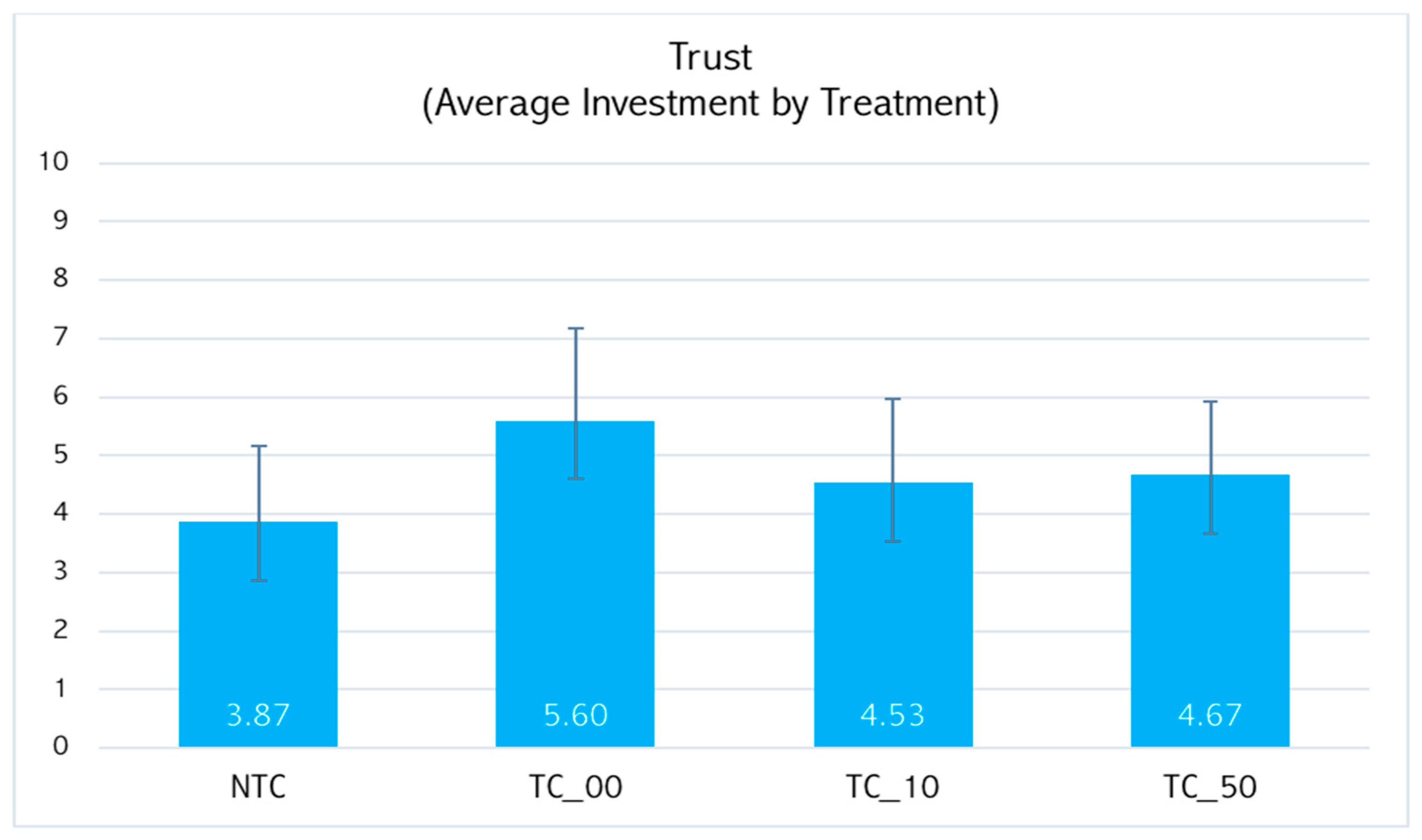
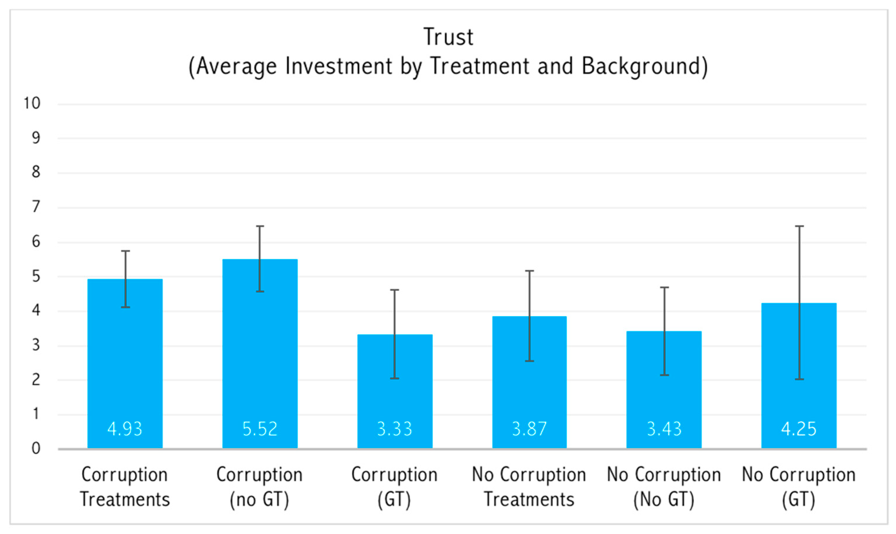
Table 1.
Balancing properties (between corruption/non-corruption treatments and players’ roles)–z-stat (with p-values in parentheses).
Table 1.
Balancing properties (between corruption/non-corruption treatments and players’ roles)–z-stat (with p-values in parentheses).
| Corruption vs. Non-Corruption Treatments | Trustors only (Corr. vs. Non-Corr. Treatments) | Trustees only (Corr. vs. Non-Corr. Treatments) | Trustor vs. Trustee | Trustor vs. Third Corrupting Agent | Trustee vs. Third Corrupting Agent | |
|---|---|---|---|---|---|---|
| Male | 0.520 (0.603) | 0.000 (1.000) | −0.148 (0.882) | 0.55 (0.585) | −1.68 (0.093) | −2.21 (0.027) |
| Age | 2.23 (0.024) | 1.771 (0.077) | −0.301 (0.764) | −0.14 (0.887) | 1.07 (0.204) | 1.27 (0.203) |
| Voluntary status | 0.53 (0.598) | −0.699 (0.485) | 1.645 (0.100) | −2.131 (0.033) | 0.029 (0.977) | 1.812 (0.070) |
| Years of education | −0.005 (0.998) | −1.330 (0.1835) | 1.481 (0.139) | −0.961 (0.343) | −0.847 (0.402) | 0.092 (0.932) |
| Risk aversion * | −1.624 (0.104) | −0.952 (0.341) | 0.027 (0.979) | −0.073 (0.941) | 0.485 (0.628) | 0.535 (0.593) |
| Game theory knowledge | 0.359 (0.730) | −1.881 (0.060) | 0.307 (0.759) | 0.381 (0.703) | 0.381 (0.703) | 0.000 (1.00) |
Non-parametric, two-sided, Mann–Whitney rank-sum test. * Self-assessed degree of risk aversion: “Using a 0–10 scale how much do you like to take risk (high return/high risk investment, extreme sports, lotteries, and other risky behavior) or try to avoid it? 0 (I try to avoid it)–10 (I like risk)”.
Table 2.
Trustor’s expectations of the withdrawal of the third agent.
| (1) | (2) | |
|---|---|---|
| S | 0.615 *** | 0.641 *** |
| (0.026) | (0.033) | |
| S × TC_10 | 0.057 | −0.008 |
| (0.037) | (0.046) | |
| S × TC_50 | 0.019 | −0.035 |
| (0.037) | (0.043) | |
| S × Game Theory | 0.421 *** | |
| (0.104) | ||
| S × TC_10 × Game Theory | −0.305 *** | |
| (0.117) | ||
| S × TC_50 × Game Theory | −0.486 *** | |
| (0.116) | ||
| Constant | 0.416 ** | 0.416 ** |
| (0.190) | (0.185) | |
| F-stat | ||
| 587.12 | 311.59 | |
| p > F | 0.00 | 0.00 |
| Observations | 450 | 450 |
| R-squared (within) | 0.814 | 0.824 |
| Number of id. | 45 | 45 |
This table reports estimates (with standard errors in parentheses) from a fixed effects regression. The dependent variable is the trustor’s expectations of the choice of the third (corrupted) agent, S is the surplus generated in the trust game played in the first two stages of the experiment. TC_10 and TC_50 are treatment dummies. Game Theory is a dummy that takes a value of 1 if the subject is reported to have knowledge of game theory in the post-experiment questionnaire. S × TC_10, S × TC_50, S × Game Theory, S × TC_10 × Game Theory, and S × TC_50 × Game Theory are interaction terms. Results remain qualitatively unchanged if replicating the analysis with either clustered standard errors to control for potential sources of dependency within session or robust bootstrapped standard errors to control for non-normality and heteroskedasticity of residuals. Significance levels are denoted as follows: *** p < 0.01, ** p < 0.05.
Table 3.
Trustor’s expectations of trustee’s strategy.
| (1) | (2) | (3) | (4) | |
|---|---|---|---|---|
| All Data | Game Theory = 1 | Game Theory = 0 | All Data | |
| 1.232 *** | 1.058 *** | 1.430 *** | 1.430 *** | |
| (0.071) | (0.091) | (0.104) | (0.102) | |
| × TC_0 | −0.252 ** | −0.327 ** | −0.284 ** | −0.284 ** |
| (0.100) | (0.139) | (0.139) | (0.136) | |
| × TC_10 | −0.266 *** | −0.304 ** | −0.359 *** | −0.359 *** |
| (0.100) | (0.147) | (0.136) | (0.133) | |
| × TC_50 | 0.036 | 0.458 * | −0.181 | −0.181 |
| (0.100) | (0.274) | (0.128) | (0.125) | |
| × Game Theory | −0.373 *** | |||
| (0.140) | ||||
| × TC_0 × Game Theory | −0.043 | |||
| (0.200) | ||||
| × TC_10 × Game Theory | 0.056 | |||
| (0.204) | ||||
| × TC_50 × Game Theory | 0.639 ** | |||
| (0.313) | ||||
| Constant | 0.373 * | 0.630 * | 0.245 | 0.373 * |
| (0.220) | (0.358) | (0.271) | (0.216) | |
| F-stat | 249.55 | 64.90 | 195.13 | 131.40 |
| p > F | (0.000) | (0.000) | (0.000) | (0.000) |
| Observations | 600 | 200 | 400 | 600 |
| R-squared | 0.651 | 0.596 | 0.687 | 0.664 |
| Number of id. | 60 | 20 | 40 | 60 |
The dependent variable is the trustor’s expectations of the choice of the trustee, is the amount sent by the trustor in the first stage of the experiment. × TC_0, × TC_10, × TC_50, × Game Theory, × TC_0 × Game Theory, × TC_10 × Game Theory, and × TC_50 × Game Theory are interaction terms. All other remarks of Table 2 apply. *** p < 0.01, ** p < 0.05, * p < 0.1.
Table 4.
The trustor’s giving, expectations, and expected return on giving.
| Expected Return on Giving | ||||
|---|---|---|---|---|
| Players who know game theory | ||||
| NTC (n = 7) | 4.25 | 1.06 | 6 percent | |
| TC_0 (n = 6) | 4.16 | 0.60 | 64 percent | Negative |
| TC_10 (n = 5) | 2.2 | 0.73 | 74 percent | Negative |
| TC_50 (n = 1) | 4 | 1.06 | 100 percent | negative |
| Players who do not know game theory | ||||
| NTC (n = 8) | 4.25 | 1.43 | 43 percent | |
| TC_0 (n = 9) | 6.55 | 1.15 | 64 percent | 5.4 percent |
| TC_10 (n = 10) | 5.7 | 1.08 | 64 percent | 2.9 percent |
| TC_50 (n = 14) | 4.71 | 1.43 | 64 percent | 15.5 percent |
Table 5.
Trustee’s expectations of the “corruption tax” (third agent’s withdrawal).
| (1) | (2) | (3) | (4) | |
|---|---|---|---|---|
| All Data | Game Theory = 1 | Game Theory = 0 | All Data | |
| S | 0.638 *** | 0.608 *** | 0.665 *** | 0.665 *** |
| (0.026) | (0.041) | (0.033) | (0.035) | |
| S × TC_10 | 0.060 | 0.142 ** | 0.014 | 0.014 |
| (0.036) | (0.067) | (0.044) | (0.046) | |
| S × TC_50 | 0.001 | −0.004 | −0.001 | −0.001 |
| (0.036) | (0.060) | (0.046) | (0.048) | |
| S × Game Theory | −0.060 | |||
| (0.052) | ||||
| S × TC_10 × Game Theory | 0.131 * | |||
| (0.078) | ||||
| S × TC_50 × Game Theory | 0.003 | |||
| (0.073) | ||||
| Constant | 0.116 | 0.427 | −0.074 | 0.116 |
| (0.184) | (0.323) | (0.221) | (0.184) | |
| F-stat | 657.19 | 203.17 | 470.22 | 330.13 |
| p > F | 0.00 | 0.00 | 0.00 | 0.00 |
| Observations | 450 | 170 | 280 | 450 |
| R-squared | 0.831 | 0.803 | 0.850 | 0.832 |
| Number of id. | 45 | 17 | 28 | 45 |
The dependent variable is the trustee’s expectations of the choice of the third (corrupted) subject in the third phase of the experiment, The dummy Game Theory now takes a value of one if the trustee reported having knowledge of game theory in the post-experiment questionnaire. All other remarks of Table 3 apply. *** p < 0.01, ** p < 0.05, * p < 0.1.
Table 6.
Trustee’s choice.
| (1) | (2) | (3) | (4) | (5) | |
|---|---|---|---|---|---|
| All Data | Game Theory = 1 | Game Theory = 0 | All Data | All Data | |
| 0.669 *** | 0.796 *** | 0.605 *** | 0.605 *** | 0.605 *** | |
| (0.057) | (0.091) | (0.069) | (0.067) | (0.071) | |
| × Game Theory | −0.191 | −0.191 | |||
| (0.117) | (0.123) | ||||
| × TC_0 | 0.248 *** | 0.052 | 0.373 *** | 0.373 *** | |
| (0.080) | (0.119) | (0.104) | (0.101) | ||
| × TC_10 | −0.107 | −0.545 *** | 0.069 | 0.069 | |
| (0.080) | (0.137) | (0.096) | (0.093) | ||
| × TC_50 | 0.422 *** | −0.014 | 0.692 *** | 0.692 *** | |
| (0.080) | (0.123) | (0.100) | (0.098) | ||
| × TC_0 × Game Theory | −0.321 * | ||||
| (0.161) | |||||
| × TC_10 × Game Theory | −0.614 *** | ||||
| (0.170) | |||||
| × TC_50 × Game Theory | 0.705 *** | ||||
| (0.162) | |||||
| × TC | 0.356 *** | ||||
| (0.083) | |||||
| × TC × Game Theory | −0.467 *** | ||||
| (0.141) | |||||
| Constant | 0.612 *** | 0.612 ** | 0.612 *** | 0.612 *** | 0.612 *** |
| (0.176) | (0.269) | (0.220) | (0.171) | (0.180) | |
| F-stat | 217.19 | 73.13 | 164.46 | 119.73 | 200.91 |
| 0.000 | 0.000 | 0.000 | 0.000 | 0.000 | |
| Observations | 600 | 220 | 380 | 600 | 600 |
| R-squared | 0.618 | 0.601 | 0.661 | 0.643 | 0.600 |
| Number of id. | 60 | 22 | 38 | 60 | 60 |
The dependent variable is the trustee’s choice in the second phase of the experiment, Game Theory is a dummy that takes a value of one if the trustee reports having knowledge of game theory in the post-experiment questionnaire. TC is a dummy that takes a value of 1 in treatments with corruption (TC_0, TC_10, and TC_50). × Game Theory,, × TC_0 × Game Theory, × TC_10 × Game Theory, × TC_50 × Game Theory, × TC, and × TC × Game Theory are interaction terms. All other remarks of Table 3 apply. *** p < 0.01.
Table 7.
Aggregate (trustors and trustees) expectations of the corruption tax.
| (1) | (2) | |
|---|---|---|
| S | 0.627 *** | 0.652 *** |
| (0.018) | (0.024) | |
| S × TC_10 | 0.058 ** | 0.005 |
| (0.026) | (0.033) | |
| S × TC_50 | 0.010 | −0.024 |
| (0.026) | (0.032) | |
| S × Game Theory | 0.035 | |
| (0.043) | ||
| S × TC_10 × Game Theory | 0.057 | |
| (0.059) | ||
| S × TC_50 × Game Theory | −0.094 * | |
| (0.057) | ||
| Constant | 0.266 ** | 0.266 ** |
| (0.132) | (0.132) | |
| F-stat | 1245.26 | 628.31 |
| p > F | (0.000) | (0.000) |
| Observations | 900 | 900 |
| R-squared | 0.822 | 0.824 |
| Number of id. | 90 | 90 |
The dependent variable is the aggregated trustor’s and trustee’s expectations of the choice of the third (corrupted) agent, All other remarks of Table 2 apply. *** p < 0.01, ** p < 0.05, * p < 0.1.
Table 8.
The behavior of the third agent (corruption tax).
| (1) | (2) | |
|---|---|---|
| S | 0.708 *** | 0.638 *** |
| (0.026) | (0.037) | |
| S × Game Theory | 0.131 *** | |
| (0.050) | ||
| S × TC_10 | 0.055 | 0.083 * |
| (0.036) | (0.048) | |
| S × TC_50 | −0.057 | −0.068 |
| (0.036) | (0.050) | |
| S × TC_10 × Game Theory | −0.006 | |
| (0.073) | ||
| S × TC_50 × Game Theory | 0.041 | |
| (0.071) | ||
| Constant | −0.201 | −0.201 |
| (0.184) | (0.180) | |
| F-stat | 759.04 | 403.48 |
| p > F | 0.000 | 0.000 |
| Observations | 450 | 450 |
| R-squared | 0.850 | 0.859 |
| Number of id. | 45 | 45 |
The dependent variable is the choice of the third (corrupted) agent in the third phase of the experiment, The dummy Game Theory now takes a value of one if the third agent reported having knowledge of game theory in the post-experiment questionnaire. All other remarks of Table 3 apply. *** p < 0.01, * p < 0.1.
Publisher’s Note: MDPI stays neutral with regard to jurisdictional claims in published maps and institutional affiliations. |
© 2021 by the authors. Licensee MDPI, Basel, Switzerland. This article is an open access article distributed under the terms and conditions of the Creative Commons Attribution (CC BY) license (http://creativecommons.org/licenses/by/4.0/).
Share and Cite
MDPI and ACS Style
Becchetti, L.; Corazzini, L.; Pelligra, V. Trust and Trustworthiness in Corrupted Economic Environments. Games 2021, 12, 16. https://0-doi-org.brum.beds.ac.uk/10.3390/g12010016
AMA Style
Becchetti L, Corazzini L, Pelligra V. Trust and Trustworthiness in Corrupted Economic Environments. Games. 2021; 12(1):16. https://0-doi-org.brum.beds.ac.uk/10.3390/g12010016
Chicago/Turabian StyleBecchetti, Leonardo, Luca Corazzini, and Vittorio Pelligra. 2021. "Trust and Trustworthiness in Corrupted Economic Environments" Games 12, no. 1: 16. https://0-doi-org.brum.beds.ac.uk/10.3390/g12010016
Note that from the first issue of 2016, this journal uses article numbers instead of page numbers. See further details here.