
Imitation and Local Interactions: Long Run Equilibrium Selection


Department of Economics and Management, University of Florence, Via Delle Pandette 9, 50127 Florence, Italy
Games 2021, 12(2), 30; https://0-doi-org.brum.beds.ac.uk/10.3390/g12020030
Submission received: 30 January 2021
/
Revised: 19 March 2021
/
Accepted: 26 March 2021
/
Published: 1 April 2021
(This article belongs to the Special Issue Social Coordination Games)
Abstract
:In this paper, we analyze the long run dynamics of a multi-agent game played on a one-dimensional lattice with periodic boundary conditions, i.e., a ring. Agents repeatedly play a 2 × 2 coordination game with neighbors where the payoff dominant action and the risk dominant action are distinct. Necessary and sufficient conditions for both the actions to be the unique long run equilibrium are provided. The result is obtained through the application of the radius and modified coradius technique.
1. Introduction
We study a model in which agents are located on a one-dimensional lattice and interact only with their neighbors. Agents play a 2 × 2 coordination game where one action is payoff dominant and the other action satisfies the risk dominant criterion of Harsanyi and Selten [1]. We find necessary and sufficient conditions for the payoff dominant action and the risk dominant action to be the unique long run equilibrium under the imitate the best-neighbor behavioral rule. For some values of the payoff matrix, both the actions belong to the set of long run equilibria. Our results are an extension of the results of Alós-Ferrer and Weidenholzer [2], in which sufficient conditions for the payoff dominant action to be the unique long run equilibrium are provided.
Coordination problems represent a consistent part of social and economic interactions. Usually coordination problems are not only related to the convergence of strategies in a population toward a convention. In fact, the problem of which convention is selected is a relevant issue when there are multiple achievable conventions. Some major examples on how a coordination problem converges to a convention are languages, standards in technological products, and the adoption of a common currency, such as EUR. Evolutionary game theory and the stochastic stability analysis offer instruments to asses which convention is selected in the long run. In this paper, we contribute to the literature finding conditions under which a convention that is payoff dominated is inefficiently selected in the long run.
The related literature is presented in Section 2. In Section 3, we present the model, while, in Section 4, we describe the unperturbed dynamics generated by the model, characterizing the absorbing states. In Section 5, we introduce a perturbation in order to perform the stochastic stability analysis. Finally, in Section 6, there are the conclusions. All the proofs are relegated in Appendix B.
2. Related Literature
A well known result in literature on evolutionary game theory is that the selected long run equilibrium in a 2 × 2 coordination game, repeatedly played in a large population, depends on the behavioral rule, the error model, and the structure of interactions. When interactions are at the global level, i.e., when players interact with each other without any restriction, the seminal papers of Kandori et al. [3] and Young [4] show that the risk dominant action is selected in the long run. In Kandori et al. [3], a subset of players has a revision opportunity in each period and best reply to the current situation. In a 2 × 2 coordination game with global interactions, the best reply behavior coincides with the imitative behavior. Noise is introduced in the dynamics at the individual level; in fact, players have a small probability to make mistakes and select the action that is not the best reply in the current situation. The long run equilibrium coincides with the state in which all the players select the action that is risk dominant, and only in the case in which the level of risk of the two actions is equal is the payoff dominant action selected. An adaptive play with bounded memory is used in Young [4]. Players collect information about the strategies performed in the near past up to a limit; in fact, the memory capacity is bounded, and new information replace the older. Players best reply to the distribution of strategies observed in the unperturbed process, while mistakes are possible when noise is introduced. Similarly to Kandori et al. [3], in 2 × 2 coordination games, the risk dominant convention is selected in the long run. Bergin and Lipman [5] show that the long run equilibria depend on the underlying specification of noise. Any absorbing state of the unperturbed process can be obtained in the long run with appropriate state-dependent mutations rates. In fact, in the previous literature, the error rate is independent from the state of the process, the agent, and the payoffs obtained in the past, while it is plausible to assume that better performing agents have less incentive to experiment, and, in general, to commit mistakes. More recently along this line of research Bilancini and Boncinelli [6] describe a model in which past payoffs determine the rate at which errors converge to zero. Moreover interactions are at the global level, but there is a positive probability that two agents remains matched for more than one period. As a result, they obtain that, when the termination probability of a matching is high enough, the maximin convention emerges in the long run. As stated above, the behavioral rule of agents also has a major impact on the determination of long run equilibria. Recent results of Sawa and Wu [7] and Nax and Newton [8] show that, in the presence of loss aversion and risk aversion, the maximin strategy is stochastically stable.
A part of the literature studies models in which interactions are at the local level. Players are located on a graph and interact only with a subset of agents, the neighbors. A main distinction in this literature is between models with exogenous fixed networks and models in which the network is endogenously generated. A recent contribution in this second strand of literature is Staudigl and Weidenholzer [9]. Players can decide both the action, of a 2 × 2 coordination game, and the neighbors to whom play. In this setting, the payoff dominant action emerges in the long run, when the number of interactions is limited, through the simple fact that a small group of players playing the payoff dominant action enables the other players to obtain the highest payoff by linking to them and playing the payoff dominant action. When, instead, the number of possible links is unlimited, and the linking cost is small enough, the risk dominant action is observed in the long run. The last case seems much closer to a global interaction model than a local interaction one.
The seminal paper of Ellison [10] proved that, under a best reply behavioral rule, the system converges towards the risk dominant equilibrium, when agents are deployed on a one dimension lattice. In addition, in Blume [11], the risk dominant equilibrium is selected when agents play a 2 × 2 coordination game with neighbors. Switching costs are introduced by Norman [12] in a framework similar to Ellison [10]. Jiang and Weidenholzer [13] develop a model in which agents are located on a ring and best reply to the strategy of the two closest neighbors. They discuss the emergence of different stochastically stable states varying the magnitude of switching costs. When switching costs are small, the risk dominant action is the unique stochastically stable state, as in Ellison [10], while, for intermediate costs, the two monomorphic states are alternately the stochastically stable state. For high values of switching costs, some non-monomorphic states also enter in the stochastically stable set. In Alós-Ferrer and Weidenholzer [14], agents follow an imitate the best behavioral rule and the spatial structure is given by a two-dimensional lattice. The payoff dominant action is selected in the long run when the information network is larger than the interaction network. A similar result is obtained by Khan [15]; in this model, interactions are at the global level, while information accessible to players is at the local level. Under an imitate the best neighbor behavioral rule, the payoff dominant action is always stochastically stable, while the risk dominant action is stochastically stable only in some special case. The payoff dominant action is the unique stochastically stable state when each player has at least four neighbors or when the information network is regular. In Cui [16], agents are located on an arbitrary network and interact with all the neighbors contemporary. The imitative behavior described is slightly different from the previous literature; in fact, an agent during a revision opportunity compares his mean payoff with the payoff obtained by a random neighbor interacting with a random neighbor’s neighbor. The payoff dominant convention is the unique stochastically stable state if the dimension of neighborhoods is big enough. In Alós-Ferrer and Weidenholzer [2], agents are deployed on one dimension lattice and in each period every agent revises the strategy imitating the neighbor obtaining the highest payoff. Sufficient conditions for the payoff dominant action to be the long run equilibrium are provided. As in Cui [16], the dimension of neighborhoods is the main driver of the result; in fact, given any possible payoff matrix of the 2 × 2 coordination game, a threshold value for the dimension of neighborhoods is obtained. If neighborhoods are larger than the threshold, the payoff dominant convention is the unique stochastically stable state. The stochastically stable set when the dimension of neighborhoods is lower than the threshold is no further analyzed. In this paper, we develop on the model of Alós-Ferrer and Weidenholzer [2], providing a fully characterization of the stochastically stable sets. Given the dimension of neighborhoods, we identify the values of the parameters of the 2 × 2 underlying coordination game for which the risk dominant convention is the unique long run equilibrium, and the values for which is instead the payoff dominant convention the unique long run equilibrium. There are also values of the parameters for which the set of long run equilibria is made by both the conventions.
3. The Model
Agents are deployed on one-dimensional lattice, i.e., a ring, and interact only with a subset of agents, the neighbors. The underlying 2 × 2 coordination game has the following payoff matrix (Table 1):
Where and so that both and are strict Nash equilibria. We assume that is payoff dominant; then, we have , and is risk dominant [1], implying that . Without losing generality, we normalize the payoff matrix (Table 2):
Where the entries are referred to the row player, and and . We constrain the analysis to the case in which .
3.1. Interaction
The neighbors are agents at distance lower or equal to k, and the neighborhood is the set of all the neighbors:
Every agent does not belong to his neighborhood, irreflexivity, and, if agent i belongs to the neighborhood of agent j, then agent j belongs to the neighborhood of agent i, symmetry. The dimension of each neighborhood is equal to , where . When , interactions are at the global level. The total payoff obtained by an agent is the sum of the payoffs obtained playing the 2 × 2 game with each neighbor.
3.2. Revision Opportunities
In every period, all the agents have a revision opportunity. Usually, in the literature, it is not necessary that all the agents revise their strategies simultaneously in each period. In that case, the probability of revision is given by a parameter that represents the level of inertia of agents. We assume to be more adherent to Alós-Ferrer and Weidenholzer [2,14].
Agents choose the action of the neighbor that, in the last period, obtains the highest payoff. If, in the last period, an agent obtained a payoff greater than the payoff of all his neighbors, then such an agent maintains the same strategy.
There is no memory, i.e., only the current situation matters, and not how it was reached. The behavior of agents is myopic, they do not take in account the possible future states. With global interactions in 2 × 2 coordination games, the imitate the best and best reply behavior coincide. When interactions are at the local level, the relationship between best reply and imitation in coordination games is broken. The imitative behavioral rule may drive the dynamics to the payoff dominant convention in the long run through costly decisions in the short run. Whenever an imitative agent chooses an action that differs from the best reply, it is paying a cost in the short run. This is a consequence of the fact that the neighborhood of a neighbor of agent i is different from the neighborhood of agent i.
4. Unperturbed Dynamics
The dynamics are completely determined, except in the case in which there are ties, which are broken randomly, including a stochastic component in the unperturbed process. A prevailing characteristic of these dynamics is the emergence of clusters of agents choosing the same action. In this section, we initially concentrate on the dimension of such clusters.
Definition 1.
A cluster is a set of adjacent agents choosing the same action.
Definition 2.
A cluster is resistant if the dimension of the cluster is not reduced by any revision opportunity.
Label the A and B neighbors with higher payoff as and , respectively. Each agent has a and a neighbor. Resistant clusters can be ordered by their dimension, namely the number of agents composing the cluster.
Definition 3.
A minimal group is a resistant cluster with minimal dimension.
When , for each agent, it is convenient to be located near to other agents doing the same action. The more are the same-action neighbors the greater is the payoff. To prove that a cluster is resistant, we need to check that the extreme agents do not change action in case of a revision opportunity. If agents on the border do not change their action, then agents in the internal part of the cluster also do not change their action; furthermore, if a cluster is resistant, a bigger cluster is also resistant. The dimension of the minimal group for action A, , is in between and . A cluster of agents A is always resistant. An A agent situated on the border of a cluster of or more A agents has a neighbor at distance k with exactly neighbors A, and such an agent obtains a payoff equal to that is the maximum possible payoff of the game.
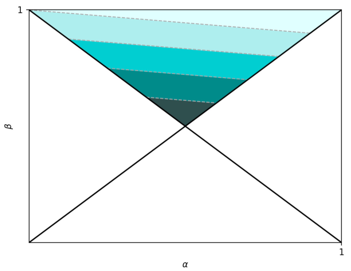
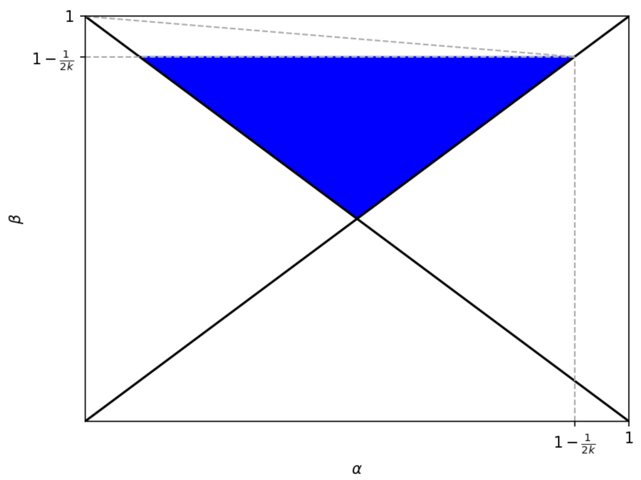
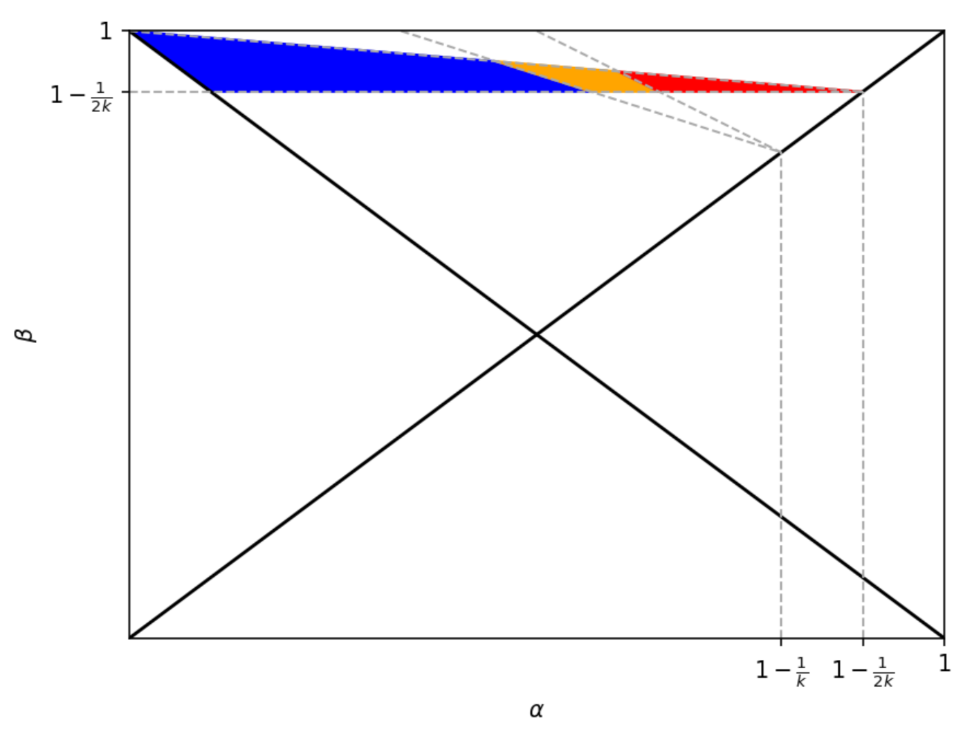
Different areas, in Figure 1, associated to different values of minimal A group dimension are obtained through parametric analysis. The bounds of areas, characterized by different dimensions of minimal A groups, consist of parallel segments with slope equal to . Areas on the top of Figure 1, lighter colors, are associated with greater values of minimal A group dimension. The fundamental point for the proof of the main propositions is that, for , is the dimension of minimal A groups, while, when , the dimension of minimal A groups is lower or equal to . The dimension of a minimal A group is equal to i when:
The dimension of the minimal group for action B is labeled with . or more B clusterized agents are not always resistant. In fact, when the dimension of minimal B groups is greater than . In this case, B groups are able to resist only when close to the monomorphic B state, i.e., the state in which all the agents play action B.
The dimension of the minimal B group, , is equal to j if:
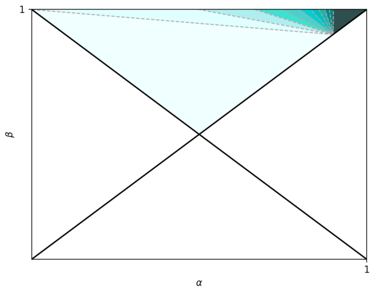
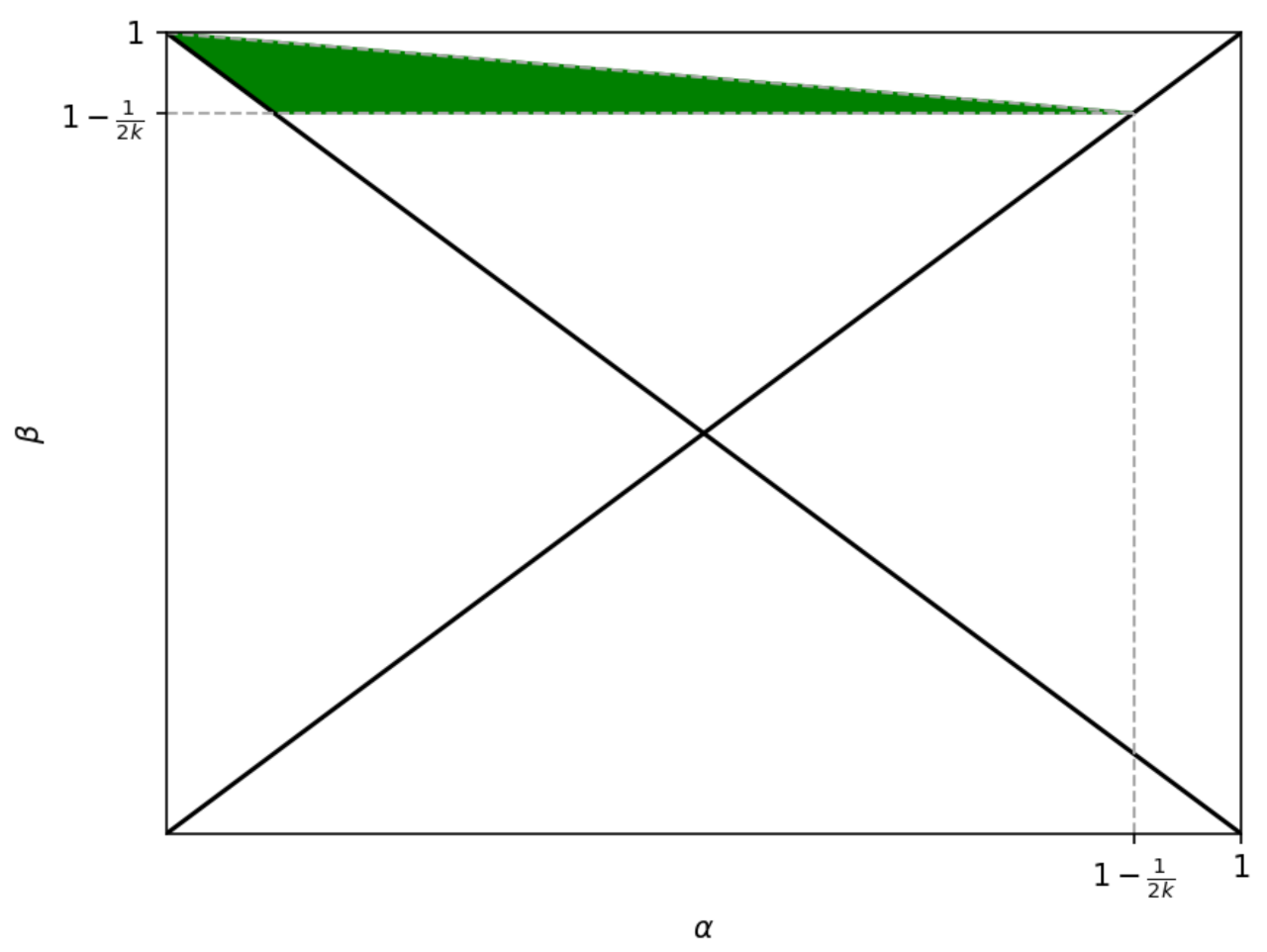
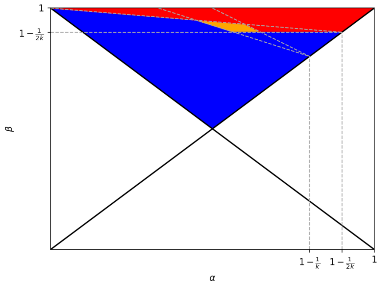
The dimension of minimal B groups varies from one to and from to . The bounds of the different areas in Figure 2 form a set of concurrent lines intersecting at point .
Absorbing States
An absorbing set is a set of states that, once reached, cannot be left, and there does not exist any proper subset with the same property. When an absorbing set is made by a single state, that is an absorbing state. In the next lemma, we give a characterization of absorbing states.
Lemma 1.
A state made of resistant clusters is an absorbing state.
An absorbing set is non-singleton when it is composed by more than one state. In this case, once the dynamics reach a state contained in the absorbing set, all and only the states of the absorbing set will be visited by the dynamics. The states belonging to a non-singleton absorbing set cannot be made of resistant clusters. In the next Lemma, we prove that there are no non-singleton absorbing sets, i.e., all the absorbing sets are made by one and only one state.
Lemma 2.
There are no non-singleton absorbing sets.
There exists a multiplicity of absorbing states of the unperturbed Markov chain, and which one is reached depends mainly on the states from which the dynamics begin. In the next section, we perform a stochastic stability analysis, selecting between the different absorbing states.
5. Stochastic Analysis
In this section, we introduce a perturbation at the individual level in order to be able to select the stochastically stable states, i.e., the states that are observed with a positive probability in the long run. The perturbation hits randomly at the individual level, making an agent choose an action different from the action of the best neighbor. The probability that such an event occurs is equal to . Since each agent has only two feasible strategies with probability , the agent chooses the strategy of the best neighbor, while, with probability , the agent chooses the other strategy. To perform the stochastic stability analysis, we use the radius-coradius technique [17]. Radius measures the persistence of an absorbing state, i.e., the difficulty to leave the basin of attraction of an absorbing state. Coradius and modified coradius are instead measures of the difficulty to reach the basin of attraction of an absorbing state, once the dynamics are in the basin of attraction of another absorbing state, see Appendix A for precise definitions. The stochastically stable set is contained in the set of absorbing states with radius greater than coradius, i.e., states for which the difficulty to leave the basin of attraction is greater than the difficulty to reach it. As we show in the previous section, there are a multiplicity of absorbing states, among which the two monomorphic states are of major interest. In the next lemma, we prove that all the absorbing states different from the two monomorphic states are not stochastically stable. In fact, these absorbing states have radius equal to one; since coradius is greater or equal to one, radius is certainly smaller or equal to coradius.
Lemma 3.
Each absorbing state, except the two monomorphic states and , has radius equal to one.
Only the two monomorphic states are possible candidates for being stochastically stable. In the next lemma, we exploit the fact that a path connecting the two monomorphic absorbing states can be traversed in both the directions.
Lemma 4.
When , we have:
The number of errors needed to leave one of the two monomorphic absorbing states represents both the radius of that state, and the modified coradius of the other monomorphic state. Then, to prove which one of the two monomorphic states is the unique long run equilibrium, we just need to calculate the radius of the two.
Notice that the radius of state , (), is lower or equal to the dimension of minimal resistant B, (A), group:
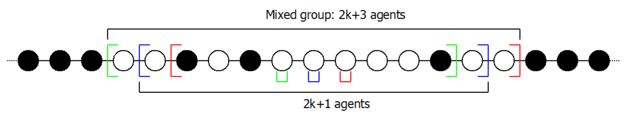
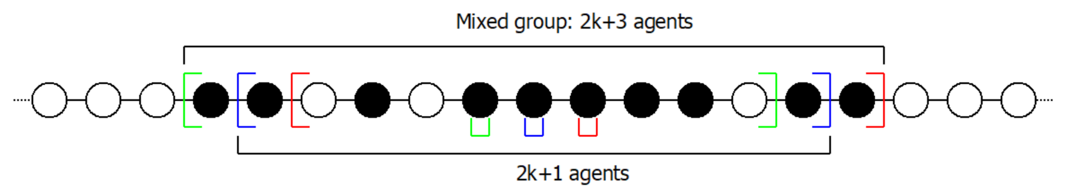
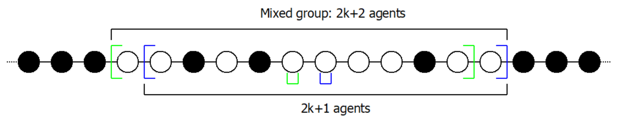
In fact, starting from the monomorphic state , (), it is hypothetically possible to generate a minimal dimension A (B) cluster with a number of errors lower or equal to (). Assume that it is possible to generate a resistant cluster of agents A, with only errors. We should have a configuration similar to the one in Figure 3, in which there is a mixed group of agents composed by agents A and a certain number of agents B. If the B agents inside the group switch to A, and not too many A agents switch to B, a resistant cluster of agents A is generated, from the monomorphic state , with only errors.
With Lemma 5, we prove that, when , the less costly way to generate a minimal dimension A cluster is to have exactly contemporaneous errors.
Lemma 5.
When , we have that:
The result of Lemma 5 is the main ingredient for the proof of Proposition 1.
Proposition 1.
In the 2k neighbors model, with , uniform perturbation and imitate the best neighbor behavior, when , the all-B monomorphic state, , is the unique stochastically stable state.
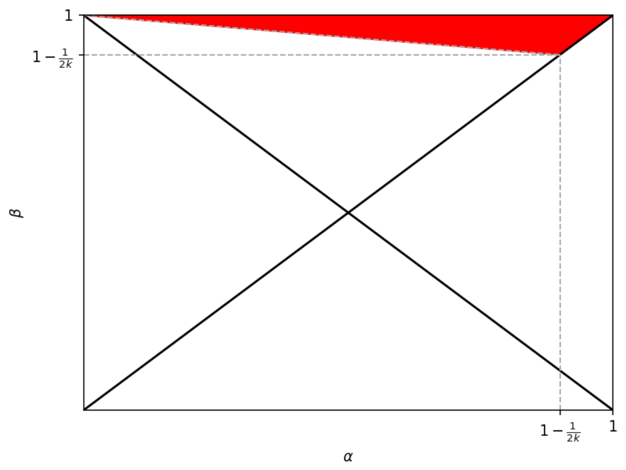
In Figure 4, we graphically represent the area in which the all-B monomorphic state, , is the unique stochastically stable state as identified in Proposition 1. Notice that, when , the condition is equivalent to , i.e., the condition under which B is the risk dominant action. Then, in this case, the all-B monomorphic state, , is always the unique long run equilibrium. This result was presented as a special case in Alós-Ferrer and Weidenholzer [2].
In Proposition 2, we find sufficient conditions for the all-A monomorphic state, , to be the unique long run equilibrium.
Proposition 2.
In the 2k neighbors model, with , uniform perturbation and imitate the best neighbor behavior, when
the all-A monomorphic state, , is the unique stochastically stable state.
In Figure 5, we graphically represent the area in which, for values of , the all-A monomorphic state is the unique long run equilibrium.
We now pass to study the long run equilibria of the system in the green area of Figure 6:
Anticipating the results, the area is divided into three parts. The unique long run equilibrium is in the first part, while it is in the second part. In the third part, both and are long run equilibria.
In the green area of Figure 6, the dimension of the minimal A group is equal to , while is the dimension of the minimal B group. Differently from A, Lemma 5, a resistant cluster of agents B can be generated with less than errors. When is the dimension of the minimal B group, the following inequalities hold:
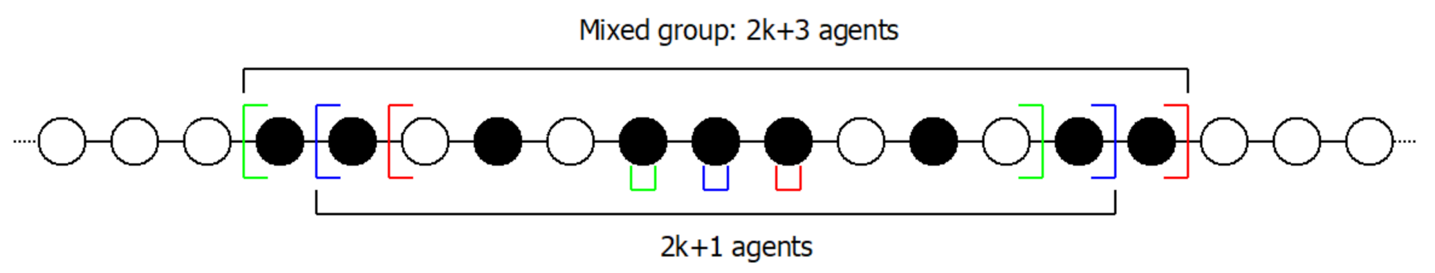
Consider a group of agents composed by or less B agents and one or more A agents such that the first and the last one are B agents, and all the agents outside the group are A agents; see Figure 7 and Figure 8.
In such a group, when , the two B agents on the border always switch to A. In fact, the payoff of the best B neighbor is equal to , while the payoff of the best A neighbor is equal to . The result follows from the first inequality in (1). At the same time, the A agents inside the group could switch to B, generating a resistant cluster of agents B.
In Lemma 6, we find the radius of the monomorphic state , and, in Lemma 7, we find the radius of the monomorphic state .
Lemma 6.
- Forthe radius of is equal to :
- Forthe radius of is lower than :
- Forthe radius of is equal to :
Lemma 7.
In area:
the radius of is equal to :
The next Proposition follows from the combination of Lemmas 6 and 7, comparing the radii of the two monomorphic states.
Proposition 3.
In the 2k neighbors model, with , uniform perturbation and imitate the best neighbor behavior, in area (green area in Figure 6):
we have:
- is the unique stochastically stable convention if
- , both belong to stochastically stable set if
- is the unique stochastically stable convention if
The results of Proposition 3 are summarized in Figure 9.
6. Conclusions
This paper analyzes a local interaction model in which agents imitate successful behaviors. We contribute to the literature on coordination games played in a large population. The selection of the risk dominant convention or the payoff dominant one depends on the details of the model. In this paper, agents are located on a one dimension lattice, i.e., a ring, and interact only with a subset of agents, the neighbors. Each agent is in the middle of his own neighborhood. In every period, all the agents revise their strategy, imitating the action of the neighbor that, in the previous period, obtains the highest payoff. Once a small and persistent perturbation is introduced in the model, it is possible to identify the long run equilibria of the dynamics, i.e., the stochastically stable states.
Merging the results of Propositions 1–3, we find necessary and sufficient conditions for both the risk dominant convention and the payoff dominant convention to be stochastically stable. The area characterized by and , implying that A is payoff dominant and B is risk dominant, can be dividend into three regions. In the first region, the payoff dominant convention is the unique long run equilibrium, while the risk dominant convention is the unique long run equilibrium in the second region. In the third region, both the conventions belong to the set of the long run equilibria. In Figure 10, we provide a graphic representation of the results. When the level of payoff dominance of action A is relatively large with respect to the level of risk dominance of action B, the payoff dominant convention, , is the unique stochastically stable state. Conversely, when the level of risk dominance is relatively larger the risk dominant convention, , it is the unique stochastically stable state. For intermediate values, both the conventions belong to the set of stochastically stable states.
The results obtained are strongly conditioned by the particular hypothesis of the model. This limitation of the paper leads the way to several future research directions. The stochastic analysis could be performed in the region in which . In this setting, agents playing the risk dominant action, B, perform better when they are isolated. This feature generates a qualitatively different dynamics. Sufficient conditions for the emergence in the long run of the payoff dominant convention in this setting are obtained by Alós-Ferrer and Weidenholzer [2]. Alternative forms of the network structure could be analyzed. This further research would be of major interest in assessing how much the main results depend on the particular network structure chosen. We expect that, in regular networks, such as a square lattice with periodic boundary conditions, i.e., a torus, there is still a tendency to the creation of clusters of agents choosing the same action, as for the ring. The major problem to extend the model in this direction is that the analytical difficulty is strongly increased by the fact that also the form of a cluster matters and not only the dimension. A promising way of addressing this issue is to simulate the model. Two recent contributions along this strand of literature are Alós-Ferrer, Buckenmaier, and Farolfi [18,19]. As discussed in Section 2, the specification of the noise determines the outcomes of the model. It is possible to argue that a uniform error model, as the one adopted in this paper, represents poorly the behavior of human players. Recent contributions find experimental evidence that different specifications of noise better fit human behavior [20,21,22,23]. In Mäs and Nax [21] and Bilancini and Boncinelli [22], two different specification of noise are tested. The first is the class of condition-dependent error models, in which a mistake made by an agent experiencing low payoffs is more likely to be observed. This class of error models well capture the idea that agents poorly performing tend to experiment more, and, in this sense, they make more errors [6]. Using such a specification of noise, not all the errors occur with the same probability; then, to calculate the cost of a transition from a state x to another state (see Equation (A1)), different errors should be weighted differently. On the one hand, moving from the definition of payoff dominance, we can argue that the risk dominant monomorphic state is more easily invaded than the payoff dominant one, suggesting an increase in the area of the parameters’ space in which the payoff dominant convention is the long run equilibrium. On the other hand, in the absorbing states that are not monomorphic, at the border between resistant clusters of agents A and B, the risk dominant agents perform better, and then experiment less, thus suggesting an increase in the area of the parameters’ space in which the risk dominant convention is the long run equilibrium. Which of the two phenomena prevails is of interest for a future research. The second class of error models is cost-dependent, meaning that costly mistakes are less likely to be done. A prominent example in this class is the logit response model [11]. With imitate the best neighbor behavior, the cost of a mistake is given by the difference in the utilities of the best-A and the best-B neighbor. In the two monomorphic states, such a comparison is impossible because all the neighborhoods are homogeneous. If we consider the utility of the other-action best neighbor equal to zero, the cost-dependent error model collapses on the condition-dependent error model. The behavioral rule of agents is a further hypothesis that can be relaxed to check the robustness of results. In the evolutionary game theory literature, different behavioral dynamics have been explored; for a review of recent contributions, see Newton [24]. The possibility that an agent follows different behavioral rules at different times, or that different agents comply to different behavioral rules at the same time, is studied recently in Newton [25]. An imitate the average best behavioral rule increases the strength of the risk dominant action in invading payoff dominant clusters, suggesting an increase in the area of the parameters’ space in which the risk dominant convention is the long run equilibrium. Different imitative rules, such as imitate the majority, completely change the results, implying that both the conventions are always stochastically stable under uniform error model, independently from payoffs.
Funding
This research received no external funding.
Institutional Review Board Statement
Not applicable.
Informed Consent Statement
Not applicable.
Conflicts of Interest
The author declares no conflict of interest.
Appendix A. Radius and Coradius
In this subsection, we present the definition of radius and modified coradius as given by Ellison [17]. Let X be the state space and P the Markov transition matrix on X. P() is the perturbed Markov transition matrix. With a uniform mistake error model, every error can occur with the same probability. P() is irreducible, i.e., from each state, it is possible to reach every other state in a finite number of steps, and, being X finite, P() is also ergodic; furthermore, . Let be the cost function:
the number of errors, probability events, necessary to move from state x to state x’.
The radius measures the persistence of an absorbing state in the perturbed process, while coradius and modified coradius measure the difficulty to reach the basin of attraction of an absorbing state having as initial condition a state outside the basin of attraction. The basin of attraction of is the set of states from which the unperturbed process, P, converges to with probability one:
The radius of is the number of probability events necessary to leave the basin of attraction of starting from . Define a path from a set of states to a set of states as a sequence of states such that at least belongs to , and only belongs to . The cost of a path is the sum of the costs of each step of the path:
Given all the paths from to any state outside , the radius of the basin of attraction of is equal to the cost of the path with minimal cost:
where is the set of all the paths from to any state outside . While the radius is a measure of the difficulty of leaving the basin of attraction of an absorbing state, the coradius is instead a measure of the difficulty with which is reached the basin of attraction of an absorbing state when the initial state is outside the basin of attraction. The path with minimal cost, connecting x and , is selected for each state x outside the basin of attraction of . Then, the coradius of is equal to the maximum cost between all the minimal cost paths:
In Reference [17], Theorem 2, the modified coradius is used instead of the coradius. To define the modified coradius, we have to define a modified cost function. The cost function of a path is the number of probability events necessary to move from one absorbing state to another one minus the radius of intermediate absorbing states, i.e., the absorbing states crossed by the path:
with the sequence of absorbing states from which the path is passing. The modified coradius of is equal to:
Appendix B. Proofs
Proof of Lemma 1.
Agents belonging to a resistant cluster do not change action. In a state made of resistant clusters, no agent changes action. Such a state is absorbing. □
Proof of Lemma 2.
Let be a state without any cluster with a dimension greater or equal to the dimension of the minimal resistant cluster. In , there are one or more agents obtaining the highest payoff, :
If M is a singleton, or there exists at least one element of M that is not sharing any neighbor with another element of M, then, in , there is at least a cluster of agents; in fact, all the neighbors of this agent copy its strategy. If two elements of M, one A and the other B, share one or more neighbors, the agents belonging to both the neighborhoods are indifferent between choosing A or B. Ties are broken randomly, then there is a positive probability that agents in between the two elements of M change action generating a cluster of same action agents. Then, from a state without any cluster with a dimension greater or equal to the dimension of the minimal resistant cluster, there is a positive probability to move in one or more periods to a state with at least a cluster of agents playing the same action.
In the second step of the proof, we show that a state with at least a cluster of agents with the same action has a positive probability to move to an absorbing state as in Lemma 1, i.e., a state made of resistant clusters. A cluster of agents is resistant; therefore, agents belonging to the cluster do not change action, and the agents on the border that join the cluster also can no longer change action. Suppose, without losing generality, that there exists in state a cluster of agents A. If the two B agents on the border switch to A when , then does not belong to an absorbing set; in fact, it is impossible to move back to state . The two B agents on the border of the cluster do not change action only if they belong to clusters with dimension greater or equal to . The same argument can be applied to the A agents on the borders of these two B clusters. Repeating the reasoning, we obtain a state as in Lemma 1. □
Proof of Lemma 3.
From every absorbing state with at least a minimal A group and a minimal B group, it is possible to reach another absorbing state with only one error at the border between the two groups.
where is the set of all the absorbing states. □
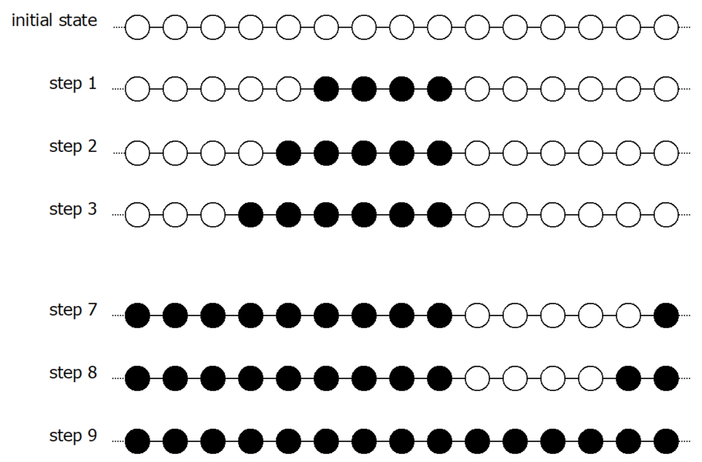
Figure A1.
Example of a minimal cost path from to . A agents are white, while B agents are black. In the example, , , and . Step 8 .
Figure A1.
Example of a minimal cost path from to . A agents are white, while B agents are black. In the example, , , and . Step 8 .

Proof of Lemma 4.
Firstly, note that () is equal to the minimal number of simultaneous errors necessary to pass from state () to a state with only one minimal dimension cluster of B (A) agents, and only A (B) agents in the rest of the population.
Second, we describe the path connecting to with minimal modified cost. The originating state of the path is ; with a number of errors equal to the system moves to a state with a minimal B group with dimension , this state is an absorbing state. Then, with only one error at the border of the cluster, the system moves to an absorbing state with clusterized B agents. The radius of such an absorbing state is equal to one (see Lemma 3), and the cost of the transition is equal to one; then, the balance in Equation (A2) is equal to zero. From this state, with another error at the border, the system reaches an absorbing state with clusterized B agents. The same procedure is repeated until the system reaches a state with agents B, where is the dimension of the minimal A group. Then, with only one error, the system enters into the basin of attraction of .
The cost of the first transition of the path is equal to . In all the steps of the remaining part of the path, the balance between the cost of the transition and the radius of the intermediate absorbing state is equal to zero. Then, we have:
The very same argument can be used to prove that:
□
Proof of Lemma 5.
To prove that, when , the less costly way to generate a minimal dimension A cluster is to have exactly contemporaneous errors, we start from the observation that, in a configuration similar to the one in Figure 3, the two external A agents always switch to B. In fact, the payoff of the best-B neighbor is always greater than the payoff of the best-A neighbor:
where is the maximal possible payoff of an agent A in a group with only agents A. The previous inequality follows from the fact that when:
Since the two A agents on the border switch to B, then, to obtain a cluster of agents A, it is necessary that three B agents inside the mixed group switch to A. A mixed group with agents A and three agents B is represented in Figure 3.
If the second and the last-second agents of the mixed group are B agents, then they do not switch to A. In fact, the payoff of the neighbor is always greater than the payoff of the neighbor:
We now show that the second and the last-second A agents always switch to B. From Figure 3, observe that the neighborhood of the neighbor of the second (and last-second) A agent is made by three agents B and agents A. The neighbor is instead outside the mixed group, with neighbors B and the remaining two neighbors A.
Then, we have that the second (and the last-second) A agent does not change action if:
which is equivalent to:
Recall that when
Then, the second and last-second A agents always switch to B. In fact, the intersection between the two inequalities (A3) and (A4) is empty.
In conclusion, a minimal cluster of agents A can be generated with at least errors. □
Proof of Proposition 1.
To prove the Proposition, we follow Theorem 2 in Reference [17]. From Lemma 5, we know that . Recall that, when , we have . Since , we get:
is the unique long run equilibrium. □
Figure A2.
Three periods of length 6.

Proof of Proposition 2.
When , the dimension of the minimal A cluster is in between and ; then, for Lemma 4:
We need now to calculate when . In this region, a cluster of agents A belongs to the basin of attraction of . In fact, consider a B agent on the border of such a cluster. Its best B neighbor has a utility lower or equal to , while the best A neighbor has a utility equal to . Since , the B agent on the border switches to A. This reasoning can be repeated until the dynamics reach the monomorphic state . The less costly way to leave the basin of attraction of , , is to disband every A cluster with at least agents.
We can consider the circle as divided into periods, and each period is equal to the others. A period is made by r agents A and one agent B in the last position from the left.
If, in a period, after one iteration, all the agents switch to B, then, to leave the basin of attraction of , we need a number of errors equal to the total number of periods, i.e., N divided by the length of periods. The shortest is the length of the period, L; the greater is the number of errors needed to leave the basin of attraction of , since the area of interest is:
A state made of periods of length , composed by A agents and a B agent, belongs to the basin of attraction of . Then, the number of errors needed to leave the basin of attraction of is greater than . This means that:
Recall from the first step of the proof that
In conclusion, when ,
and is the unique long run equilibrium. □
Proof of Lemma 6.
Consider a group of agents composed by agents B and three A agents such that the first and the last one are B agents, and all the agents outside the group are A agents, as in Figure 7. The two B agents on the border always switch to A. If the second and the second-last agents are A agents, the payoff of is equal to , greater than the payoff of . If the second and the second-last are B agents and remain B, and the three A agents switch to B, then a resistant cluster is generated with only errors. is the payoff of , while payoff is equal to . When
it is not possible to generate a resistant cluster with less than errors. In conclusion:
When, instead, , we have . Consider a group of agents composed by agents A and four B agents such that the first and the last one are B agents, and all the agents outside the group are A agents, as in Figure 8. The B agents on the border switch to A. The payoff of the and the neighbors of the second agent is, respectively, and . When
a resistant B cluster of is generated with errors, then
When, instead, , and , we have □
Figure A3.
Example of a mixed group composed by agents A and three B agents such that the first and the last one are A agents, and all the agents outside the group are B agents. .
Figure A3.
Example of a mixed group composed by agents A and three B agents such that the first and the last one are A agents, and all the agents outside the group are B agents. .

Proof of Lemma 7.
To prove that the less costly way to generate a cluster of agents A is to have exactly contemporaneous errors, we start from the observation that, in a configuration similar to the one in Figure A3, the two external A agents always switch to B; in fact:
holds in the green area of Figure 6. The second and the last-second A agents do not switch if
or equivalently if
While they switch otherwise. In conclusion, when
is impossible to generate a minimal A cluster of agents with less than errors, in fact, restricting the analysis to the green area in Figure 6, the intersection between inequalities (A5) and (A6) is empty. Then,
□
Proof of Proposition 3.
In the area of interest, . When
, then:
is the unique long run equilibrium. When, instead,
, then:
is the unique long run equilibrium. In the third area:
and let .
□
References
- Harsanyi, J.C.; Selten, R. A General Theory of Equilibrium Selection in Games; MIT Press: Cambridge, MA, USA, 1988; Volume 1. [Google Scholar]
- Alós-Ferrer, C.; Weidenholzer, S. Imitation, local interactions, and efficiency. Econ. Lett. 2006, 93, 163–168. [Google Scholar] [CrossRef]
- Kandori, M.; Mailath, G.J.; Rob, R. Learning, mutation, and long run equilibria in games. Econometrica 1993, 61, 29–56. [Google Scholar] [CrossRef]
- Young, H.P. The evolution of conventions. Econometrica 1993, 61, 57–84. [Google Scholar] [CrossRef]
- Bergin, J.; Lipman, B.L. Evolution with state-dependent mutations. Econometrica 1996, 64, 943–956. [Google Scholar] [CrossRef] [Green Version]
- Bilancini, E.; Boncinelli, L. The evolution of conventions under condition-dependent mistakes. Econ. Theory 2019, 69, 497–521. [Google Scholar] [CrossRef] [Green Version]
- Sawa, R.; Wu, J. Prospect dynamics and loss dominance. Games Econ. Behav. 2018, 112, 98–124. [Google Scholar] [CrossRef]
- Nax, H.H.; Newton, J. Risk attitudes and risk dominance in the long run. Games Econ. Behav. 2019, 116, 179–184. [Google Scholar] [CrossRef]
- Staudigl, M.; Weidenholzer, S. Constrained interactions and social coordination. J. Econ. Theory 2014, 152, 41–63. [Google Scholar] [CrossRef] [Green Version]
- Ellison, G. Learning, local interaction, and coordination. Econometrica 1993, 61, 1047–1071. [Google Scholar] [CrossRef] [Green Version]
- Blume, L.E. The statistical mechanics of strategic interaction. Games Econ. Behav. 1993, 5, 387–424. [Google Scholar] [CrossRef] [Green Version]
- Norman, T.W. Rapid evolution under inertia. Games Econ. Behav. 2009, 66, 865–879. [Google Scholar] [CrossRef] [Green Version]
- Jiang, G.; Weidenholzer, S. Local interactions under switching costs. Econ. Theory 2017, 64, 571–588. [Google Scholar] [CrossRef] [Green Version]
- Alós-Ferrer, C.; Weidenholzer, S. Contagion and efficiency. J. Econ. Theory 2008, 143, 251–274. [Google Scholar] [CrossRef]
- Khan, A. Coordination under global random interaction and local imitation. Int. J. Game Theory 2014, 43, 721–745. [Google Scholar] [CrossRef] [Green Version]
- Cui, Z. More neighbors, more efficiency. J. Econ. Dyn. Control 2014, 40, 103–115. [Google Scholar] [CrossRef]
- Ellison, G. Basins of attraction, long-run stochastic stability, and the speed of step-by-step evolution. Rev. Econ. Stud. 2000, 67, 17–45. [Google Scholar] [CrossRef] [Green Version]
- Alós-Ferrer, C.; Buckenmaier, J.; Farolfi, F. Imitation, network size, and efficiency. Netw. Sci. 2020, 9, 123–133. [Google Scholar] [CrossRef]
- Alós-Ferrer, C.; Buckenmaier, J.; Farolfi, F. When Are Efficient Conventions Selected in Networks? J. Econ. Dyn. Control 2021, 124, 104074. [Google Scholar] [CrossRef]
- Lim, W.; Neary, P.R. An experimental investigation of stochastic adjustment dynamics. Games Econ. Behav. 2016, 100, 208–219. [Google Scholar] [CrossRef]
- Mäs, M.; Nax, H.H. A behavioral study of “noise” in coordination games. J. Econ. Theory 2016, 162, 195–208. [Google Scholar] [CrossRef] [Green Version]
- Bilancini, E.; Boncinelli, L.; Nax, H.H. What noise matters? Experimental evidence for stochastic deviations in social norms. J. Behav. Exp. Econ. 2021, 90, 101626. [Google Scholar] [CrossRef]
- Hwang, S.H.; Lim, W.; Neary, P.; Newton, J. Conventional contracts, intentional behavior and logit choice: Equality without symmetry. Games Econ. Behav. 2018, 110, 273–294. [Google Scholar] [CrossRef] [Green Version]
- Newton, J. Evolutionary game theory: A renaissance. Games 2018, 9, 31. [Google Scholar] [CrossRef] [Green Version]
- Newton, J. Conventions under Heterogeneous Behavioural Rules. Rev. Econ. Stud. 2020, 0, 1–25. [Google Scholar]
Figure 1.
Areas characterized by different dimension of minimal A groups. Areas on the top, lighter colors, are associated with greater values of minimal A group dimension.
Figure 1.
Areas characterized by different dimension of minimal A groups. Areas on the top, lighter colors, are associated with greater values of minimal A group dimension.

Figure 2.
Areas characterized by different dimension of minimal B groups. Areas on the top, darker colors, are associated with lower values of minimal B group dimension.
Figure 2.
Areas characterized by different dimension of minimal B groups. Areas on the top, darker colors, are associated with lower values of minimal B group dimension.

Figure 3.
Example of a group composed by agents A and three B agents such that the first and the last one of the group are A agents, and all the agents outside the group are B agents. , A agents are white, and B agents are black.
Figure 3.
Example of a group composed by agents A and three B agents such that the first and the last one of the group are A agents, and all the agents outside the group are B agents. , A agents are white, and B agents are black.

Figure 4.
In the red area, the all-B monomorphic state is the unique long run equilibrium.

Figure 5.
In the blue area, the all-A monomorphic state is the unique long run equilibrium, when .

Figure 6.
In the green area, the dimension of the minimal A group is equal to , while is the dimension of the minimal B group.
Figure 6.
In the green area, the dimension of the minimal A group is equal to , while is the dimension of the minimal B group.

Figure 7.
Example of a mixed group composed by agents B and three A agents such that the first and the last one of the group are B agents, and all the agents outside the group are A agents. .
Figure 7.
Example of a mixed group composed by agents B and three A agents such that the first and the last one of the group are B agents, and all the agents outside the group are A agents. .

Figure 8.
Example of a mixed group composed by agents B and four A agents such that the first and the last one of the group are B agents, and all the agents outside the group are A agents. .
Figure 8.
Example of a mixed group composed by agents B and four A agents such that the first and the last one of the group are B agents, and all the agents outside the group are A agents. .

Figure 9.
In the red area, is the unique long run equilibrium; in the blue area, is the unique long run equilibrium; in the orange area, both and are long run equilibria.
Figure 9.
In the red area, is the unique long run equilibrium; in the blue area, is the unique long run equilibrium; in the orange area, both and are long run equilibria.

Figure 10.
In the red area, is the unique long run equilibrium; in the blue area, is the unique long run equilibrium; in the orange area, both and are long run equilibria.
Figure 10.
In the red area, is the unique long run equilibrium; in the blue area, is the unique long run equilibrium; in the orange area, both and are long run equilibria.


Table 1.
Payoff matrix.
| A | B | |
|---|---|---|
| A | ||
| B |
Table 2.
Normalized payoff matrix.
| A | B | |
|---|---|---|
| A | 1 | 0 |
| B |
Publisher’s Note: MDPI stays neutral with regard to jurisdictional claims in published maps and institutional affiliations. |
© 2021 by the author. Licensee MDPI, Basel, Switzerland. This article is an open access article distributed under the terms and conditions of the Creative Commons Attribution (CC BY) license (https://creativecommons.org/licenses/by/4.0/).
Share and Cite
MDPI and ACS Style
Vicario, E. Imitation and Local Interactions: Long Run Equilibrium Selection. Games 2021, 12, 30. https://0-doi-org.brum.beds.ac.uk/10.3390/g12020030
AMA Style
Vicario E. Imitation and Local Interactions: Long Run Equilibrium Selection. Games. 2021; 12(2):30. https://0-doi-org.brum.beds.ac.uk/10.3390/g12020030
Chicago/Turabian StyleVicario, Eugenio. 2021. "Imitation and Local Interactions: Long Run Equilibrium Selection" Games 12, no. 2: 30. https://0-doi-org.brum.beds.ac.uk/10.3390/g12020030
Note that from the first issue of 2016, this journal uses article numbers instead of page numbers. See further details here.