Cooperative Game for Fish Harvesting and Pollution Control

Abstract

This paper studies fishery strategies in lakes, seas, and shallow rivers subject to agricultural and industrial pollution. The flowing pollutants are modeled by a nonlinear differential equation in a general manner. The logistic growth model for the fish population is modified to cover the pollution impact on the fish growth rate. We start by presenting the stability analysis of the dynamical system to discern the different types of the evolution of the fish population according to human actions. A cooperative game is formulated to design strategies for preserving the fish population by controlling the pollution as well as the fish stock for harvesting. The sufficient conditions for implementing the cooperative strategy are investigated through an incentive design approach with an adaptive taxation policy for the players. Numerical results are presented to illustrate the benefit of the cooperative for fish population preservation but also for the players’ rewards.

1. Introduction

Prior to the 2019 coronavirus disease (COVID-19) pandemic, towns and cities had grown and attracted more than fifty percent of the world population. Their sustainability and competitive efficiency have become increasingly important issues to decision-makers. A city, more simply, is a geographic area where live people, with hard infrastructures and changing systems that interconnect the city with itself. Because of pandemics, economic drivers, energy, climate change, and resource supply, the concept of biodiversity preservation has gained more attention for the next generation of cities, called smart cities. The “smart city” can include a large and extensive range of systems, networks, and infrastructure elements. However, in this paper we use the term “smart city” to refer to more intelligent, more efficient, and more sustainable cities, and we focus on pollution control and economic supply. In support of the environment, risk management and sustainable development; natural resource management including systems for the reduction of pollutants; increasing energy efficiency; managing the human response to environmental stresses, and sustaining biodiversity are key elements of smart cities.

Seas and lakes provide a variety of economic uses: they are sources of drinking water, fishing, and recreational sports, and they provide pleasant locations for smart homes and drainage for agriculture. Runoff from fields flows into the streams and rivers that feed the lake. Much of the agricultural runoff includes phosphorus from fertilizers and animal wastes. Phosphorus is the primary nutrient of algae and weeds in the water. When it grows excessively from an infusion of phosphorus, algae blooms reduce the oxygen content of the lake and release toxins into the water. In addition, large amounts of waste produced by some industries and municipal sewage enter natural water bodies, either without treatment or through inappropriate and inadequate treatment processes [1]. In fact, the sources of water pollution are various [2]. Seas and lakes are polluted with high concentrations of phosphorus, Pb, Zn, Cu, Cd, and other toxins in their sediments. This pollution severely affects aquatic life and leads to a serious environmental, climatic, and public health problem. Fish and other marine species die due to high levels of pesticides and toxins in water and other types of water pollution, such as plastic and litter [3]. On the other hand, fish reproduction is seriously affected because of genetic mutations when toxins are absorbed. Fish are therefore mainly affected by human nuisance and it is necessary to give sufficient attention to this issue and to implement the necessary corrective measures [3,4].

Research activities are focused on finding suitable solutions to these problems. Anupam et al. [5] proposed a new mathematical model that uses fuzzy inferences to study the impacts of global warming, water pollution, and juvenile fish harvesting on the production of mature Hilsa fish. They used the Mamdani inference method and applied it to a model based on fuzzy rules. Most recent mathematical models take into account the spatialization of fisheries to study the control of a multi-site fishery [6]. For this, bio-economic models can be used. These models take into account economic aspects and, in particular, changes in investment and prices, in fisheries management models [7]. It is possible to eliminate over-fishing and move towards a sustainable fishery without risk of extinction for the exploited species, by varying the number of fishing sites and the costs of operating the fishery [8]. For a more recent work on economic models, see [9], where the authors studied the dynamics of marine industrial interactions through a dynamical systems theory approach.

For pollution control, the authors in [10] considered a dynamic partial equilibrium model that combines the optimum exploitation of renewable resources with optimum pollution control. For them, the pollution accumulates as a slowly decomposing stock and is supposed to affect the growth and quality of the stock of renewable resources. They maximized a social welfare function that gives the present value of the difference between the benefits of natural resources and the costs of controlling pollution. Their analysis also gives a general result concerning the state of equilibrium of two problems of optimal control. In [11], a mathematical model for solving the dispersion of pollutants in a river is considered. The concentration of the pollutant is obtained using a finite element method. This is subject to optimal control of the water treatment plants in order to achieve minimum costs.

In this paper, we introduce a mathematical model describing the impact of pollution on the fish population. The pollution dynamic covers the time unit input of chemical residuals and the eutrophication process; see [12]. The dynamic of the fish population is obtained by discharging the harvested fish stock from the natural logistic growth model. The in-water part of the allowed portion, according to the regulations, of the fishable population is referred to as the “fish stock” [13]. To gain clarity in the mathematical analysis, we first study the properties of the eutrophication dynamics. Moreover, considering fish preservation, we investigate the gain optimization for polluters and fishermen in non-cooperative and cooperative regimes. Two separate payoff functions are defined in the non-cooperative regime, while a single aggregated payoff for all the players is considered in the cooperative regime under the authority of a third entity. It is revealed that the cooperative regime is more supportive of fish preservation.

The outline of the paper is as follows: in Section 2, we discuss the management problem to develop the mathematical model. Section 3 is dedicated to the mathematical analysis, which is based on the basic reproduction number of the eutrophication dynamics. The non-cooperative optimization between the polluters and the fishermen with the constraint of preserving the fish population is presented in Section 4. In Section 5, we address the cooperative optimization and present sufficient conditions for its implementation.

2. Water Pollution and Fishing Industry

In this section, we describe the management problem of ecosystem preservation, present the mathematical models for the pollution and the fish population, and identify the control variables.

2.1. Management Problema

We identify the first class of players: farmers and mining industries surrounding rivers, lakes, and seas are polluters. Industry companies need to clean up material or deposit chemical waste into the water. Farmers use artificial fertilizers to grow crops; these fertilizers contain chemical elements such as phosphorus and zinc, which are ultimately washed out into the water. The dynamic of the chemical waste (such as the amount of phosphorus in the water) is given by [12,14]:

$$\begin{array}{c}\hfill {\dot{x}}_{{}_1}\left(t\right)=\sum _{j=1}^n{a}_j\left(t\right)-c{x}_{{}_1}\left(t\right)+b\frac{x_{{}_1}^p\left(t\right)}{x_{{}_1}^p\left(t\right)+m^p}.\end{array}$$

Here, n is the total number of polluters (farming and industrial companies); $a_j$ is the input of chemical waste (due to industrial production and farming) produced by the player j; $c\ge 0$ is proportional to the rate of loss of chemical elements due to the sedimentation, the outflow, and the sequestration in other biomasses. The term $b\frac{x_{{}_1}^p}{x_{{}_1}^p+m^p}$ ($p\ge 2,b>0$) models the production of chemicals in the water because the dissolution process generates other types of chemicals through reactions between water components and the spilled chemical.

Fishes represent the second class of players. To illustrate the dynamics and the impact of the fishing industry, we consider that the fish population size evolves according to:

$$\begin{array}{c}\hfill {\dot{x}}_{{}_2}\left(t\right)=h_{{}_1}(x_{{}_1}\left(t\right),x_{{}_2}\left(t\right))-h_{{}_2}\left(x_{{}_2}\left(t\right)\right),\end{array}$$

where the first term $h_{{}_1}$ is the inflow and the second term $h_{{}_2}$ is the outflow due to harvesting activities. We agree that the function $h_{{}_2}$ is essentially the harvesting activity as the natural death rate is neglected and we interpret the term $h_{{}_1}$ as the drift of the logistic growth model [6], i.e.,

$$\begin{array}{c}\hfill h_{{}_1}(x_{{}_1}\left(t\right),x_{{}_2}\left(t\right))=r{x}_{{}_2}\left(t\right)\left(\frac{K\left(x_{{}_1}\left(t\right)\right)-x_{{}_2}\left(t\right)}{K\left(x_{{}_1}\left(t\right)\right)}\right).\end{array}$$

The carrying capacity K is non-increasing with the pollution level $x_{{}_1}$, while the natural growth rate r is taken to be constant. If $h_{{}_1}>h_{{}_2}$, then the fish population growth continues, and for $h_{{}_1}<h_{{}_2}$, the harvesting activities are at over-fishing levels that lead to the extinction of the fish population.

2.2. Mathematical Model

The resulting ecosystem from the above problem consists of two predators (polluters and fishermen) and a single prey (fish population). The polluters are indirect predators because they do not have a direct interest in the fish population, but their activities are harmful for the fish population and can cause the fish population’s extinction. The fishermen are the direct predators for the fish population but they are naturally concerned with its preservation. If the watercourse is polluted, the fish population drops to the lowest level through $K\left(x_{{}_1}\right)$. The fish industry will lose considerable profit because the harvesting cost becomes higher and the utility (the price of fish in the market) smaller due to the low quality. Thus, a smarter solution, addressed in this paper, is to design a policy for the fish industry that may obtain a better outcome by cooperating with the farmers to control the pollution level. In this way, the farmers may be compensated by a tax reduction.

We consider $h_{{}_2}=x_{{}_2}^2{u}_{{}_2}$, where $u_2$ measures the fish stock to be harvested. Accordingly, the dynamics of the fishery subject to industrial and agricultural pollution is:

$$\begin{array}{c}\hfill \left\{\begin{array}{c}{\displaystyle {\dot{x}}_{{}_1}\left(t\right)=u_{{}_1}\left(t\right)-c{x}_{{}_1}\left(t\right)+b\frac{x_{{}_1}^p\left(t\right)}{x_{{}_1}^p\left(t\right)+m^p},}\hfill \\ {\displaystyle {\dot{x}}_{{}_2}\left(t\right)=r{x}_{{}_2}\left(t\right)\left(\frac{K\left(x_{{}_1}\left(t\right)\right)-x_{{}_2}\left(t\right)}{K\left(x_{{}_1}\left(t\right)\right)}\right)-x_2{\left(t\right)}^2{u}_{{}_2}\left(t\right),}\hfill \\ {\displaystyle x_{{}_1}(t=0)=x_{{}_1}^0\mathrm{and}{x}_{{}_2}(t=0)=x_{{}_2}^0,}\hfill \end{array}\right.\end{array}$$

(1)

where $u_{{}_1}\left(t\right)={\sum }_{j=1}^n{a}_j\left(t\right)$ globalizes the actions of the n polluters to lighten the notation. Then, the dynamical system (1) can be recast in the condensed form:

$$\begin{array}{c}\hfill \dot{x}\left(t\right)=f(x\left(t\right),u\left(t\right)),\mathrm{starting}\mathrm{at}x\left(0\right)=x^0.\end{array}$$

(2)

where the vector $u=(u_{{}_1},u_{{}_2})$ describes the players’ activities. Short-term suspension of the players’ activities appears to be insufficient to restore the fish population because, for $u_{{}_1}=u_{{}_2}=0$, the residual chemicals continue to jeopardize the natural growth of the fish population through eutrophication.

3. Analysis of the Model

This section is devoted to the stability analysis of the system (1). We start by addressing the stability of the eutrophication dynamics in a more general setting, which facilitates the stability analysis of the system, which is considered without chemical input and fishery activities, i.e., $u_{{}_1}=u_{{}_2}=0,$

$$\begin{array}{c}\hfill \left\{\begin{array}{c}{\displaystyle {\dot{x}}_{{}_1}\left(t\right)=k\left(x_{{}_1}\left(t\right)\right)x_{{}_1}\left(t\right),\mathrm{where}k\left(x_{{}_1}\right)\stackrel{\mathrm{def}}{=}-c+\frac{b{x}_{{}_1}^{{}^{p-1}}}{x_{{}_1}^{{}^p}+m^{{}^p}},\forall x_{{}_1}^p\ge 0}\hfill \\ {\displaystyle {\dot{x}}_{{}_2}\left(t\right)=r{x}_{{}_2}\left(t\right)-\frac{r{x}_{{}_2}^2\left(t\right)}{K\left(x_{{}_1}\left(t\right)\right)},}\hfill \\ x_{{}_1}\left(0\right)=x_{{}_1}^0\mathrm{and}{x}_{{}_2}\left(0\right)=x_{{}_2}^0,(x_{{}_1}^0,x_{{}_2}^0)\in {\mathbb{R}}_{+}^2.\hfill \end{array}\right.\end{array}$$

(3)

For this, we primarily focus on the analysis of the eutrophication process, which is the first equation of (3), and secondly, we end with the analysis of the complete dynamics.

3.1. Stability Analysis of the Eutrophication Process

Here, we consider the dynamics of the pollutant, described by the following nonlinear equation:

$$\begin{array}{c}\hfill \left\{\begin{array}{c}{\displaystyle {\dot{x}}_{{}_1}\left(t\right)=k\left(x_{{}_1}\left(t\right)\right)x_{{}_1}\left(t\right),}\hfill \\ \\ x_{{}_1}\left(0\right)=x_{{}_1}^0\in {\mathbb{R}}_{+},\hfill \end{array}\right.\mathrm{where}k\left(x_{{}_1}\right)\stackrel{\mathrm{def}}{=}-c+\frac{b{x}_{{}_1}^{{}^{p-1}}}{x_{{}_1}^{{}^p}+m^{{}^p}},\forall x_{{}_1}^p\ge 0\end{array}$$

(4)

with $m>0$ and the integer $p\ge 2$. Remark that the mapping $x_{{}_1}\mapsto k\left(x_{{}_1}\right)x_{{}_1}+c{x}_{{}_1}$ is nonnegative and increasing for $x_{{}_1}\in {\mathbb{R}}_{+}$, which implies that the semi-flow generated by (4) is monotone with respect to the initial conditions in ${\mathbb{R}}_{+}$. In this sequel, we will denote by $t\mapsto X(t,x_{{}_1}^0)$ the unique solution of the Cauchy problem (4) with data $x_{{}_1}^0$. The monotonicity of (4), for two initial conditions, $x_{{}_a}$ and $x_{{}_b}$, is given by:

$$\begin{array}{c}\hfill 0\le x_{{}_a}\le x_{{}_b}⟹X(t,x_{{}_a})\le X(t,x_{{}_b}),\forall t\ge 0.\end{array}$$

(5)

To establish the causality of the function k on the existence of the equilibrium points and their asymptotic behaviors, we look at the variation of k and find that k is increasing on $[0,x_{{}_1}^{🟉}]$ and decreasing on $[x_{{}_1}^{🟉},+\infty )$, where $x_{{}_1}^{🟉}=m{(p-1)}^{\frac{1}{p}}$ is the global maximum of k

$$\begin{array}{c}\hfill \underset{x_{{}_1}\in {\mathbb{R}}_{+}}{max}k\left(x_{{}_1}\right)=k\left(x_{{}_1}^{🟉}\right)=-c+\frac{b}{mp}{(p-1)}^{1-\frac{1}{p}}\mathrm{while}k\left(0\right)=-c\mathrm{and}\underset{x_{{}_1}\to +\infty }{lim}k\left(x_{{}_1}\right)=-c.\end{array}$$

We now introduce the basic reproduction number ${\mathcal{R}}_0$ of the chemical eutrophication process:

$${\mathcal{R}}_0\stackrel{\mathrm{def}}{=}\frac{b}{mpc}{(p-1)}^{1-\frac{1}{p}}.$$

(6)

In contrast to the epidemiological approach of defining ${\mathcal{R}}_0$ as an amplification factor—see [15,16]—we assign to ${\mathcal{R}}_0$ the rate of generating new chemical components as a result of the reactions between the components during eutrophication. We note that $k\left(x_{{}_1}^{🟉}\right)=c({\mathcal{R}}_0-1)$; thus, for ${\mathcal{R}}_0<1$, the total amount of generated chemicals during eutrophication is less than the number of involved input chemicals. If ${\mathcal{R}}_0>1$, the eutrophication tends to increase the amount and the number of chemicals, while ${\mathcal{R}}_0=1$ means that the toxicity level, given by the amount of residual chemicals, stays constant because it is not affected by the eutrophication. We enumerate the equilibrium points of (4) according to ${\mathcal{R}}_0$.

Proposition 1.

The number of equilibrium points of the eutrophication dynamics (4) is given by ${\mathcal{R}}_0$ as follows:

• If ${\mathcal{R}}_0<1$, the only stationary point is the free-pollution equilibrium $x_{{}_1}^{\circ }=0$.
• If ${\mathcal{R}}_0=1$, additional to the free-pollution equilibrium $x_{{}_1}^{\circ }=0$, there is one equilibrium point $x_{{}_1}^{🟉}$, which is positive.
• If ${\mathcal{R}}_0>1$, additional to the free-pollution equilibrium $x_{{}_1}^{\circ }$, there are two equilibrium points $x_{{}_1}^{⯀}$ and $x_{{}_1}^{▸}$, which are positive. For $p=2$, they are given by:

  $$\begin{array}{c}\hfill x_{{}_1}^{⯀}=\frac{b-\sqrt{b^2-4c^2{m}^2}}{2c}and{x}_{{}_1}^{▸}=\frac{b+\sqrt{b^2-4c^2{m}^2}}{2c}.\end{array}$$

It is clear that the pollution-free equilibrium $x_{{}_1}^{\circ }=0$ is always a stationary solution of (4). Furthermore, the other equilibrium of (4) is obtained by solving $k\left(x_{{}_1}\right)=0$ in $\mathbb{R}$. Indeed, using the variation of k stated earlier in this section, we observe that the graph of k intersects the abscissa $x_{{}_1}=0$ once at $x_{{}_1}^{🟉}$ when ${\mathcal{R}}_0=1$ and twice at $x_{{}_1}^{⯀}$ and $x_{{}_1}^{▸}$ when ${\mathcal{R}}_0>1$.

The following lemmas concern the behavior of the equilibrium points given in Proposition 1. In fact, Lemma 2 states that when ${\mathcal{R}}_0<1$, the pollution-free equilibrium $x_{{}_1}^{\circ }$ is globally asymptotically stable. The case ${\mathcal{R}}_0=1$ is given in Lemma 3. In this latter case, the dynamics converges to $x_{{}_1}^{\circ }$ or $x_{{}_1}^{🟉}$ whether the initial condition is in $(0,x_{{}_1}^{🟉})$ or in $(x_{{}_1}^{🟉},+\infty )$. When ${\mathcal{R}}_0>1$, we have in Lemma 4 that $x_{{}_1}^{⯀}$ is a uniform repeller. In addition, the dynamics converges to $x_{{}_1}^{\circ }$ or $x_{{}_1}^{▸}$ whether the initial condition is in $(0,x_{{}_1}^{⯀})$ or in $(x_{{}_1}^{⯀},+\infty )$.

Lemma 2.

If ${\mathcal{R}}_0<1$, then the pollution-free equilibrium point is globally asymptotically stable. Moreover, for initial state $x_{{}_1}^0>0$, the mapping $t\mapsto X(t,x_0)$ is exponentially decreasing at the rate of $c(1-{\mathcal{R}}_0)$, i.e.,

$$\begin{array}{c}\hfill 0<X(t,x_{{}_1}^0)\le x_{{}_1}^{0}exp\left(-c(1-{\mathcal{R}}_0)t\right)\forall t\ge 0.\end{array}$$

(7)

Proof. 

Let us consider a positive initial condition $x_{{}_1}^0>0$; we use the monotonicity property (5) with $x_{{}_a}=0$ and $x_{{}_b}=x_{{}_1}^0$ to show that the solution $t\mapsto X(t,x_{{}_1}^0)$ satisfies:

$$\begin{array}{c}\hfill X(t,0)\le X(t,x_{{}_1}^0)⟹0\le X(t,x_{{}_1}^0),\forall t\ge 0,\end{array}$$

since 0 is an equilibrium point.

Moreover, we have

$$\begin{array}{c}\hfill \dot{X}(t,x_{{}_1}^0)=k\left(x_{{}_1}\right)X(t,x_{{}_1}^0)\le \underset{x_{{}_1}\in {\mathbb{R}}_{+}}{max}k\left(x_{{}_1}\right)X(t,x_{{}_1}^0)=k\left(x_{{}_1}\right)X(t,x_{{}_1}^0)=c({\mathcal{R}}_0-1)X(t,x_{{}_1}^0).\end{array}$$

In short, we have $\dot{X}(t,x_{{}_1}^0)\le c({\mathcal{R}}_0-1)X(t,x_{{}_1}^0)<0$ for all $t\ge 0$, and for ${\mathcal{R}}_0<1$; this means $0<X(t,x_{{}_1}^0)\le x_{{}_1}^{0}exp\left(-c(1-{\mathcal{R}}_0)t\right)$ for all $t\ge 0$. □

Lemma 3.

If ${\mathcal{R}}_0=1$, the notion of stability is weakened because there is no basin of attraction covering the neighborhood of any two equilibrium points. However, the following properties hold:

(1) 

For all $x_{{}_1}^0\in (0,x_{{}_1}^{🟉})$, the solution $t\mapsto X(t,x_{{}_1}^0)$ is decreasing and $X(t,x_{{}_1}^0)\to x_{{}_1}^{\circ }$ as $t\to +\infty$.

(2) 

For all $x_{{}_1}^0\in (x_{{}_1}^{🟉},+\infty )$, the solution $t\mapsto X(t,x_{{}_1}^0)$ is decreasing and $X(t,x_{{}_1}^0)\to x_{{}_1}^{🟉}$ as $t\to +\infty$.

Proof. 

We recall that when ${\mathcal{R}}_0=1$, the global maximum of k is attained at $x_{{}_1}^{🟉}$, which is also an equilibrium of the dynamical system (4), i.e.,

$$\begin{array}{c}\hfill \dot{X}(t,x_{{}_1}^{🟉})=X(t,x_{{}_1}^{🟉})k\left(x_{{}_1}^{🟉}\right)=cX(t,x_{{}_1}^{🟉})({\mathcal{R}}_0-1)=0\mathrm{and}X(t,x_{{}_1}^{🟉})=x_{{}_1}^{🟉}.\end{array}$$

For an initial condition $x_{{}_1}^0\in ]0,x_{{}_1}^{🟉}]$, the monotonicity property (5) applied to $x_{{}_a}=x_{{}_1}^{\circ }$, $x_{{}_b}=x_{{}_1}^0$ and to $x_{{}_a}=x_{{}_1}^0$, $x_{{}_b}=x_{{}_1}^{🟉}$ gives us:

$$\begin{array}{c}\hfill 0=X(t,x_{{}_1}^{\circ })\le X(t,x_{{}_1}^0)\le X(t,x_{{}_1}^{🟉})=x_{{}_1}^{🟉}\forall t\ge 0,\end{array}$$

which, because the function k is increasing in ${\mathbb{R}}_{+}$, implies that:

$$\begin{array}{c}\hfill -c=k\left(0\right)\le k\left(X(t,x_{{}_1}^0)\right)\le k\left(x_{{}_1}^{🟉}\right)=0,\forall t\ge 0.\end{array}$$

Multiplying by $0\le X(t,x_{{}_1}^0)\le X(t,x_{{}_1}^{🟉})$, we find that:

$$\begin{array}{c}\hfill 0\le X(t,x_{{}_1}^0)k\left(X(t,x_{{}_1}^0)\right)\le X(t,x_{{}_1}^{🟉})k\left(x_{{}_1}^{🟉}\right)=0,\forall t\ge 0,\end{array}$$

which implies that:

$$\begin{array}{c}\hfill 0\le \dot{X}(t,x_{{}_1}^0)\le \dot{X}(t,x_{{}_1}^{🟉})=0,\forall t\ge 0.\end{array}$$

This shows that the mapping $t\mapsto X(t,x_{{}_1}^0)$ is decreasing, and since it is bounded from below by the pollution-free equilibrium $x_{{}_1}^{\circ }$, we have $X(t,x_{{}_1}^0)\to x_{{}_1}^{\circ }=0$ as $t\to +\infty$.

For an initial condition greater than $x_{{}_1}^{🟉}$, $x_{{}_1}^0>x_{{}_1}^{🟉}$, it yields from the monotonicity condition (5) with $x_{{}_a}=x_{{}_1}^{🟉}$, $x_{{}_b}=x_{{}_1}^0$ that:

$$\begin{array}{c}\hfill x_{{}_1}^{🟉}=X(t,x_{{}_1}^{🟉})<X(t,x_{{}_1}^0),\forall t\ge 0\end{array}$$

and since k is decreasing in $(x_{{}_1}^{🟉},+\infty )$, we obtain:

$$\begin{array}{c}\hfill k\left(X(t,x_{{}_1}^0)\right)<k\left(x_{{}_1}^{🟉}\right)=0,\forall t\ge 0.\end{array}$$

Multiplying by $0<x_{{}_1}^{🟉}<X(t,x_{{}_1}^0)$, we obtain:

$$\begin{array}{c}\hfill \dot{X}(t,x_{{}_1}^0)=X(t,x_{{}_1}^0)k\left(X(t,x_{{}_1}^0)\right)<0,\forall t\ge 0,\end{array}$$

which means $t\mapsto X(t,x_{{}_1}^0)$ is decreasing since it is bounded from below by the equilibrium $x_{{}_1}^{🟉}$. We conclude that $X(t,x_{{}_1}^0)\to x_{{}_1}^{🟉}$ as $t\to +\infty$. □

Lemma 4.

If ${\mathcal{R}}_0>1$, then $x_{{}_1}^{\mathrm{⯀}}$ is a uniform repeller and we have the following properties:

(1) 

For all $x_{{}_1}^0\in (0,x_{{}_1}^{\mathrm{⯀}})$, the solution $t\mapsto X(t,x_{{}_1}^0)$ is decreasing and $X(t,x_{{}_1}^0)\to x_{{}_1}^{\circ }$ as $t\to +\infty$.

(2) 

The solution $t\mapsto X(t,x_{{}_1}^0)$ is increasing if $x_{{}_1}^0\in (x_{{}_1}^{\mathrm{⯀}},x_{{}_1}^{▸})$ and decreasing if $x_{{}_1}^0\in (x_{{}_1}^{▸},+\infty )$. Moreover, $X(t,x_{{}_1}^0)\to x_{{}_1}^{▸}$ as $t\to +\infty$ for all $x_{{}_1}^0\in (x_{{}_1}^{\mathrm{⯀}},+\infty )$.

It is worth mentioning that the fact that $x_{{}_1}^{\mathrm{⯀}}$ is a repeller, for ${\mathcal{R}}_0>1$, is a consequence of (1) and (2). It is therefore sufficient to prove (1) and (2). However, the proof of (1) is similar to that of Lemma 3; therefore, we elaborate only the proof of (2). We will do so stepwise, by considering first the initial conditions in $[x_{{}_1}^{\mathrm{⯀}},x_{{}_1}^{▸}]$ and then those in $(x_{{}_1}^{▸},+\infty )$.

Proof. 

Note that the global maximum of k, given by $x_{{}_1}^{🟉}=m{(p-1)}^{\frac{1}{p}}$, satisfies $x_{{}_1}^{\mathrm{⯀}}<x_{{}_1}^{🟉}<x_{{}_1}^{▸}$. Then, for initial condition $x_{{}_1}^0\in [x_{{}_1}^{\mathrm{⯀}},x_{{}_1}^{▸}]$, either $x_{{}_1}^0\in [x_{{}_1}^{\mathrm{⯀}},x_{{}_1}^{🟉}]$ or $x_{{}_1}^0\in [x_{{}_1}^{🟉},x_{{}_1}^{▸}]$. For $x_{{}_1}^0\in [x_{{}_1}^{\mathrm{⯀}},x_{{}_1}^{🟉}]$, we apply the monotonicity property (5) to $x_{{}_a}=x_{{}_1}^{\mathrm{⯀}}$, $x_{{}_b}=x_{{}_1}^0$ and to $x_{{}_a}=x_{{}_1}^0$, $x_{{}_b}=x_{{}_1}^{🟉}$, to obtain:

$$\begin{array}{c}\hfill x_{{}_1}^{\mathrm{⯀}}=X(t,x_{{}_1}^{\mathrm{⯀}})<X(t,x_{{}_1}^0)<X(t,x_{{}_1}^{🟉}),\forall t\ge 0.\end{array}$$

Using the fact that the function k is increasing in $(x_{{}_1}^{\mathrm{⯀}},x_{{}_1}^{🟉})$, we obtain:

$$\begin{array}{c}\hfill 0=k\left(x_{{}_1}^{\mathrm{⯀}}\right)<k\left(X(t,x_{{}_1}^0)\right)<k\left(X(t,x_{{}_1}^{🟉})\right),\forall t\ge 0.\end{array}$$

By arguing similarly for $x_{{}_1}^0\in [x_{{}_1}^{🟉},x_{{}_1}^{▸}]$ and using the fact that the function k is decreasing in $(x_{{}_1}^{🟉},x_{{}_1}^{▸})$, we have:

$$\begin{array}{c}\hfill 0=k\left(x_{{}_1}^{▸}\right)<k\left(X(t,x_{{}_1}^0)\right)<k\left(X(t,x_{{}_1}^{🟉})\right),\forall t\ge 0.\end{array}$$

Multiplying the terms of the previous inequality by $0<X(t,x_{{}_1}^0)$, we obtain in both cases:

$$\begin{array}{c}\hfill 0<X(t,x_{{}_1}^0)k\left(X(t,x_{{}_1}^0)\right)=\dot{X}(t,x_{{}_1}^0),\forall t\ge 0,\end{array}$$

meaning that $t\mapsto X(t,x_{{}_1}^0)$ is increasing since it is bounded from above by $x_{{}_1}^{▸}$. This implies that $X(t,x_{{}_1}^0)\to x_{{}_1}^{▸}$ as $t\to +\infty$.

For an initial condition greater than $x_{{}_1}^{▸}$, $x_{{}_1}^0>x_{{}_1}^{▸}$, it yields from the monotonicity condition (5) with $x_{{}_a}=x_{{}_1}^{▸}$, $x_{{}_b}=x_{{}_1}^0$ that:

$$\begin{array}{c}\hfill x_{{}_1}^{▸}=X(t,x_{{}_1}^{▸})<X(t,x_{{}_1}^0),\forall t\ge 0.\end{array}$$

Since k is decreasing in $(x_{{}_1}^{▸},+\infty )\subset (x_{{}_1}^{🟉},+\infty )$, we obtain:

$$\begin{array}{c}\hfill 0=k\left(x_{{}_1}^{▸}\right)>k\left(X(t,x_{{}_1}^0)\right),\forall t\ge 0\end{array}$$

Hence, $t\mapsto X(t,x_{{}_1}^0)$ is decreasing and bounded from below by the equilibrium $x_{{}_1}^{▸}$. Therefore, $X(t,x_{{}_1}^0)\to x_{{}_1}^{▸}$ as $t\to +\infty$. □

3.2. Stability Analysis of the Fish Pollution Dynamic

Here, we focus on the analysis of the dynamical system (3), i.e.,

$$\begin{array}{c}\hfill \left\{\begin{array}{c}{\displaystyle {\dot{x}}_{{}_1}\left(t\right)=k\left(x_{{}_1}\left(t\right)\right)x_{{}_1}\left(t\right),\mathrm{where}k\left(x_{{}_1}\right)\stackrel{\mathrm{def}}{=}-c+\frac{b{x}_{{}_1}^{{}^{p-1}}}{x_{{}_1}^{{}^p}+m^{{}^p}},\forall x_{{}_1}^p\ge 0}\hfill \\ {\displaystyle {\dot{x}}_{{}_2}\left(t\right)=r{x}_{{}_2}\left(t\right)-\frac{r{x}_{{}_2}^2\left(t\right)}{K\left(x_{{}_1}\left(t\right)\right)},}\hfill \\ x_{{}_1}\left(0\right)=x_{{}_1}^0\mathrm{and}{x}_{{}_2}\left(0\right)=x_{{}_2}^0,(x_{{}_1}^0,x_{{}_2}^0)\in {\mathbb{R}}_{+}^2,\hfill \end{array}\right.\end{array}$$

(8)

where K is a non-increasing function of $x_{{}_1}\left(t\right)$. The following results give the equilibrium points related to the fish pollution dynamic. These points are obtained by combining the equilibrium points of the eutrophication process (Section 3.1) with the equilibrium points of the second equation of Equation (8), which are $x_{{}_2}^{\circ }=0$ and ${\overline{x}}_{{}_2}=K\left({\overline{x}}_{{}_1}\right)$, where ${\overline{x}}_{{}_1}$ is $x_{{}_1}^{\circ }$, $x_{{}_1}^{🟉}$, $x_{{}_1}^{\mathrm{⯀}}$ or $x_{{}_1}^{▸}$.

Proposition 5.

The number of equilibrium points of the fish pollution dynamics (8) depends on ${\mathcal{R}}_0$ as follows:

• If ${\mathcal{R}}_0<1$, the only equilibrium points are thetrivial equilibrium and the best-case scenario equilibrium, which are given, respectively, by:

  $$E_0=(x_{{}_1}^{\circ },0)=(0,0)and{E}_1=(x_{{}_1}^{\circ },K\left(x_{{}_1}^{\circ }\right))=(0,1).$$
• If ${\mathcal{R}}_0=1$, additional to the trivial equilibrium and the best-case scenario equilibrium, there are two equilibrium points, which are:

  $$E_2=(x_{{}_1}^{🟉},0)and{E}_3=(x_{{}_1}^{🟉},K\left(x_{{}_1}^{🟉}\right)).$$
• If ${\mathcal{R}}_0>1$, additional to the trivial equilibrium and the best-case scenario equilibrium, there are four equilibrium points, which are:

  $$E_4=(x_{{}_1}^{\mathrm{⯀}},0),E_5=(x_{{}_1}^{\mathrm{⯀}},K\left(x_{{}_1}^{\mathrm{⯀}}\right)),E_6=(x_{{}_1}^{▸},0)and{E}_7=(x_{{}_1}^{▸},K\left(x_{{}_1}^{▸}\right)).$$

Here, $x_{{}_1}^{\circ }$, $x_{{}_1}^{🟉}$, $x_{{}_1}^{\mathrm{⯀}}$ and $x_{{}_1}^{▸}$ are given in Proposition (1).

Since the second equation of (8) is a Bernoulli differential equation, we consider the following Lemma, which will be used together with the results of Section 3.1 to analyze the fish pollution dynamics.

Lemma 6.

Let $v\in C([0,+\infty ),{\mathbb{R}}_{+})$ be a given continuous function and $w\in C^1([0,+\infty ),{\mathbb{R}}_{+})$ the solution of the following Bernoulli differential equation:

$$\left\{\begin{array}{c}\dot{w}\left(t\right)=rw\left(t\right)-\frac{r}{K\left(v\right(t\left)\right)}{w}^2\left(t\right),t>0\hfill \\ w\left(0\right)=w_0\in {\mathbb{R}}_{+}.\hfill \end{array}\right.$$

(9)

If v is a monotone function with $v\left(t\right)\to v^{*}$ as $t\to +\infty$, then, for each $w_0>0$, we have:

$$\underset{t\to +\infty }{lim}w\left(t\right)=K\left(v^{*}\right).$$

Proof. 

The solution to the Bernoulli differential equation is:

$$w\left(t\right)={\displaystyle \frac{w_0}{{\displaystyle e^{-r(t-t_0)}+w_0{\int }_{t_0}^t\frac{r}{K\left(v\right(s\left)\right)}{e}^{-r(t-s)}ds}}},\forall t\ge t_0,$$

(10)

We recall that K is a non-increasing function of $v\left(t\right)$. As $v\left(t\right)\to v^{*}$, $K\left(v\left(t\right)\right)\to K\left(v^{*}\right)$. Let $ϵ>0$ be given and fixed. Then, there exists $t_0\ge 0$ such that $K\left(v^{*}\right)\le K\left(v\left(t\right)\right)<K\left(v^{*}\right)+ϵ$ for all $t\ge t_0$.

Hence, for all $t\ge t_0$, we have:

$${\displaystyle \frac{w_0}{{\displaystyle e^{-r(t-t_0)}+w_0{\int }_{t_0}^t\frac{r}{K\left(v^{*}\right)+ϵ}{e}^{-r(t-s)}ds}}}\le w\left(t\right)\le {\displaystyle \frac{w_0}{{\displaystyle e^{-r(t-t_0)}+w_0{\int }_{t_0}^t\frac{r}{K\left(v^{*}\right)}{e}^{-r(t-s)}ds}}}.$$

This gives:

$$K\left(v^{*}\right)\le \underset{t\to +\infty }{lim\; inf}w\left(t\right)\le \underset{t\to +\infty }{lim\; sup}w\left(t\right)\le K\left(v^{*}\right)+ϵ$$

Since $ϵ$ is arbitrary, we obtain that $w\left(t\right)\to K\left(v^{*}\right)$ as $t\to +\infty$. □

We have now all the technical elements in order to completely describe the asymptotic behavior of the solutions of (8). In the following, we refer to $E_2$, $E_4$ and $E_6$ as extinction-fish equilibrium and $E_1$, $E_3$, $E_5$ and $E_7$ as persistent-fish equilibrium. Furthermore, $E_7$ will be called the worst-case scenario equilibrium.

Next, we list in a series of lemmas the results concerning the asymptotic behavior of the system (8) in terms of the threshold ${\mathcal{R}}_0$. Lemma 8 states that when ${\mathcal{R}}_0<1$, the best-case scenario equilibrium $E_1$ is globally asymptotically stable. When ${\mathcal{R}}_0=1$ (Lemma 8), the extinction-fish equilibrium $E_2$ is unstable while the dynamics of the system converges either to the best-case scenario equilibrium $E_1$ or to the persistent-fish equilibrium $E_3$ depending on the initial condition. For the case ${\mathcal{R}}_0>1$ (Lemma 9), the extinction-fish equilibrium $E_4$ and $E_6$ are unstable. In this case, the dynamics of the system converges either to the best-case scenario equilibrium $E_1$ or to the worst-case scenario equilibrium $E_7$ depending also on the initial condition.

Lemma 7.

If $(x_{{}_1}^0,x_{{}_2}^0)\in {\mathbb{R}}_{+}\times {\mathbb{R}}_{+}^{*}$, then the fish is uniformly persistent. More precisely, there exists $\delta >0$ such that for each $(x_{{}_1}^0,x_{{}_2}^0)\in {\mathbb{R}}_{+}\times {\mathbb{R}}_{+}^{*}$, we have:

$$\underset{t\to +\infty }{lim}{x}_{{}_2}\left(t\right)\ge \delta .$$

Proof. 

Let $(x_{{}_1}^0,x_{{}_2}^0)\in {\mathbb{R}}_{+}\times {\mathbb{R}}_{+}^{*}$ be given. Using the results of Section 3.1, we know that, independently of ${\mathcal{R}}_0$, $t\to x_{{}_1}\left(t\right)$ is monotone and converges to some $\kappa$, where $\kappa$ is either $x_{{}_1}^{\circ }$, $x_{{}_1}^{🟉}$, $x_{{}_1}^{*}$ or $x_{{}_1}^{▸}$. Therefore, we deduce from Lemma 6 that $x_{{}_2}\left(t\right)\to K\left(\kappa \right)$ as $t\to +\infty$. The proof is completed. □

Lemma 8.

If ${\mathcal{R}}_0<1$, then the best-case scenario equilibrium $E_1$ is globally asymptotically stable in ${\mathbb{R}}_{+}\times {\mathbb{R}}_{+}^{*}$. More precisely, for each $(x_{{}_1}^0,x_{{}_2}^0)\in {\mathbb{R}}_{+}\times {\mathbb{R}}_{+}^{*}$, we have:

$$\underset{t\to +\infty }{lim}{x}_{{}_1}\left(t\right)=0and\underset{t\to +\infty }{lim}{x}_{{}_2}\left(t\right)=1.$$

Proof. 

Let $(x_{{}_1}^0,x_{{}_2}^0)\in {\mathbb{R}}_{+}\times {\mathbb{R}}_{+}^{*}$ be given. If ${\mathcal{R}}_0<1$, then, from Lemma 2, $t\mapsto x_{{}_1}\left(t\right)$ is monotone and converges to 0 as $t\to +\infty$. Thus, Lemma 6 implies that $x_{{}_2}\left(t\right)\to K\left(0\right)=1$ as $t\to +\infty$. □

Lemma 9.

If ${\mathcal{R}}_0=1$, then the extinction-fish equilibrium $E_2=(x_{{}_1}^{🟉},0)$ is unstable and we have the following properties:

(i) 

For each $(x_{{}_1}^0,x_{{}_2}^0)\in {\mathbb{R}}_{+}\times {\mathbb{R}}_{+}^{*}$ with $x_{{}_1}^0\in (0,x_{{}_1}^{🟉})$, we have:

$$\underset{t\to +\infty }{lim}{x}_{{}_1}\left(t\right)=0and\underset{t\to +\infty }{lim}{x}_{{}_2}\left(t\right)=1$$

i.e., $t\mapsto (x_{{}_1}\left(t\right),x_{{}_2}\left(t\right))$ converges to the best-case scenario equilibrium $E_1$.

(ii) 

For each $(x_{{}_1}^0,x_{{}_2}^0)\in {\mathbb{R}}_{+}\times {\mathbb{R}}_{+}^{*}$ with $x_{{}_1}^0\in [x_{{}_1}^{🟉},+\infty )$, we have:

$$\underset{t\to +\infty }{lim}{x}_{{}_1}\left(t\right)=x_{{}_1}^{🟉}and\underset{t\to +\infty }{lim}{x}_{{}_2}\left(t\right)=K\left(x_{{}_1}^{🟉}\right).$$

i.e., $t\mapsto (x_{{}_1}\left(t\right),x_{{}_2}\left(t\right))$ converges to the persistent-fish equilibrium $E_3$.

Proof. 

The fact that $E_2=(x_{{}_1}^{🟉},0)$ is unstable is a consequence of (i) and (ii). The proof of (i) follows the same lines of the proof of Lemma 8 and thus we only prove (ii). Let $(x_{{}_1}^0,x_{{}_2}^0)\in {\mathbb{R}}_{+}\times {\mathbb{R}}_{+}^{*}$ with $x_{{}_1}^0\in [x_{{}_1}^{🟉},+\infty )$ be given. Then, Lemma 3 ensures that $t\mapsto x_{{}_1}\left(t\right)$ is monotone and converges to $x_{{}_1}^{🟉}$ as $t\to +\infty$. Hence, we infer from Lemma 6 that:

$$\underset{t\to +\infty }{lim}{x}_{{}_2}\left(t\right)=K\left(x_{{}_1}^{🟉}\right).$$

□

The proof of the next lemma uses the same arguments of the proofs of Lemmas 7–9.

Lemma 10.

If ${\mathcal{R}}_0>1$, then the extinction-fish equilibrium $E_4=(x_{{}_1}^{\mathrm{⯀}},0)$ and $E_6=(x_{{}_1}^{▸},0)$ are unstable and we have the following properties:

(i) 

For each $(x_{{}_1}^0,x_{{}_2}^0)\in {\mathbb{R}}_{+}\times {\mathbb{R}}_{+}^{*}$ with $x_{{}_1}^0\in (0,x_{{}_1}^{\mathrm{⯀}})$, we have:

$$\underset{t\to +\infty }{lim}{x}_{{}_1}\left(t\right)=0and\underset{t\to +\infty }{lim}{x}_{{}_2}\left(t\right)=1$$

i.e., $t\mapsto (x_{{}_1}\left(t\right),x_{{}_2}\left(t\right))$ converges to the best-case scenario equilibrium $E_1$.

(ii) 

For each $(x_{{}_1}^0,x_{{}_2}^0)\in {\mathbb{R}}_{+}\times {\mathbb{R}}_{+}^{*}$ with $x_{{}_1}^0\in (x_{{}_1}^{\mathrm{⯀}},+\infty )$, we have:

$$\underset{t\to +\infty }{lim}{x}_{{}_1}\left(t\right)=x_{{}_1}^{▸}and\underset{t\to +\infty }{lim}{x}_{{}_2}\left(t\right)=K\left(x_{{}_1}^{▸}\right)$$

i.e., $t\mapsto (x_{{}_1}\left(t\right),x_{{}_2}\left(t\right))$ converges to the worst-case scenario equilibrium $E_7$.

3.3. Numerical Illustrations

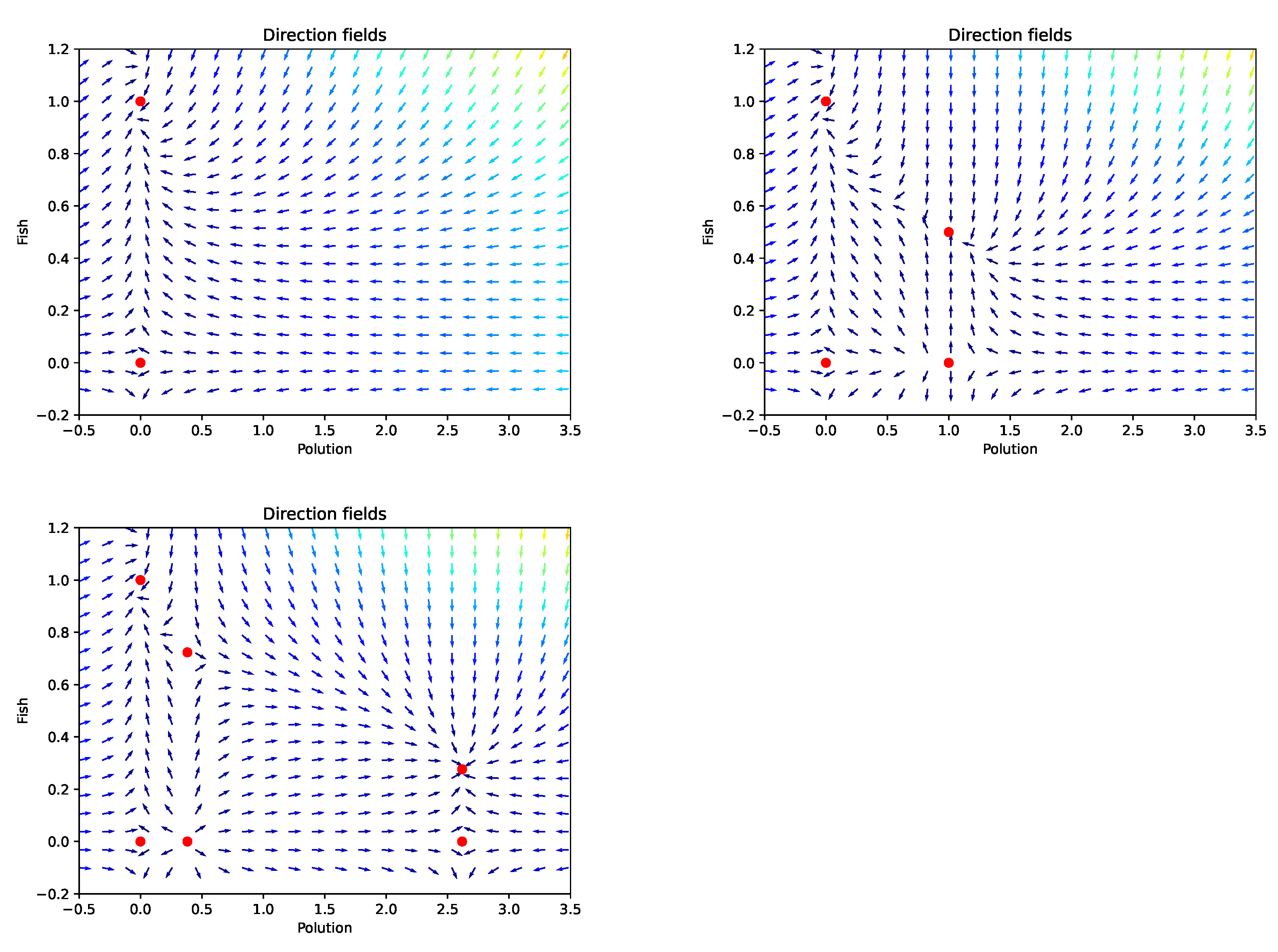
For illustration, we consider the capacity function $K\left(x_{{}_1}\right)=\frac{1}{x_{{}_1}+1}$ and the following values: $p=2$, $m=1$, $c=1$, and $r=1$. Therefore, the value of ${\mathcal{R}}_0$ will depend on b. For $b=0.7,2$ and 3, we have ${\mathcal{R}}_0=0.35<1$, ${\mathcal{R}}_0=1$ and ${\mathcal{R}}_0=1.5>1$, respectively. The dynamic of the model is given in Figure 1.

As stated in Proposition 5, the number of equilibrium points depends on ${\mathcal{R}}_0.$

• ${\mathcal{R}}_0<1.$ We have the trivial equilibrium $E_0=\left(0,0\right)$ and the best-case scenario equilibrium $E_1=\left(0,1\right)$, which is a nodal sink and globally asymptotically stable. It characterizes non-pollution for a perfect natural growth of the fish population.
• ${\mathcal{R}}_0=1$. Here, additionally to the trivial equilibrium$E_0$ and the best-case scenario equilibrium $E_1$, we have $E_2=(x_{{}_1}^{🟉},0)=(1,0)$, which is unstable, and $E_3=(x_{{}_1}^{🟉},K\left(x_{{}_1}^{🟉}\right))=(1,1/2)$. In this case, we see that if the initial condition $x_{{}_1}^0$ is in $(0,1)$, the dynamic converges to $E_1$ as stated by Lemma 9. For initial condition $x_{{}_1}^0$ starting at $x_{{}_1}=1$, $E_3$ is a stable point and behaves as a nodal sink. The level of pollution is damping at half the level of fish population growth.
• ${\mathcal{R}}_0>1$. Additionally to the trivial equilibrium$E_0$ and best-case scenario equilibrium $E_1$, we have $E_4=(x_{{}_1}^{\mathrm{⯀}}=0.38,0)$, $E_5=(x_{{}_1}^{\mathrm{⯀}}=0.38,K\left(x_{{}_1}^{\mathrm{⯀}}\right))$, $E_6=(x_{{}_1}^{▸}=2.62,0)$ and $E_7=(x_{{}_1}^{▸}=2.62,K\left(x_{{}_1}^{▸}\right))$. The equilibrium point $E_5$ is unstable (as well as $E_4$ and $E_6$) and behaves as a source. This stands for a very low pollution state, where the pollutants are not yet damping or at least not at an alarming level regarding the fish population growth. The stationary point $E_7$ is a nodal sink and is locally asymptotically stable. It illustrates the impact of a high level of pollution on the fish population. This leads asymptotically to the survival of the fish population after the total disintegration of the pollutant.

The main issue that we address in this paper is to design a fishing/pollution policy that satisfies all parties. The outcome is to have the best positioning of the stable (asymptotically stable) stationary point for both fishermen and polluters and to be able to bring and/or maintain the system state around this equilibrium. Before designing this stability policy, we must determine the feasibility, i.e., the controllability issue.

3.4. Controllability

In the rest of the paper, we consider $u_{{}_1}$ and $u_{{}_2}$ as control variables and we intend to investigate their optimal dynamics to preserve the fish population and to generate a consistent gain for both of the players in terms of business outcomes. Here, we look at the feasibility of designing such dynamics for $u_{{}_1}$ and $u_{{}_2}$ by investigating the controllability of the model. The feasibility of a mutually beneficial strategy for all the players agrees with the controllability of system (2). The first-order controllability around an equilibrium point implies its short-term controllability. In this sense, we announce the condition for the fish population preservation policy as a controllability result.

Proposition 11.

The regulation of the total pollution $u_{{}_1}$ is a necessary and sufficient condition on the feasibility of the stability policy.

Proof. 

The linear tangent system of (2) around the equilibrium point $(x^{*},u^{*})$ is given by:

$$\begin{array}{c}\hfill \dot{y}=Ay+Bu,\end{array}$$

(11)

where

$$\begin{array}{c}\hfill A={\nabla }_{x}f{{|}_{x=x^{*},u=u^{*}}\mathrm{and}B=(B_1,B_2)={\nabla }_{u}f|}_{x=x^{*},u=u^{*}}.\end{array}$$

We denote by ${\mathcal{C}}_1$, ${\mathcal{C}}_2$ and $\mathcal{C}$ the Kalman controllability matrices of (11) with respect to $u_{{}_1}$, $u_{{}_2}$ and $u$, respectively. They are given by:

$$\begin{array}{ccc}& & {\mathcal{C}}_1=\left[B_1\right|A{B}_1]=\left(\begin{array}{cc}1& -c+\frac{2b{x}_{{}_1}}{{(x_{{}_1}^2+1)}^2}\\ \\ 0& -r{x}_{{}_2}^2\end{array}\right),\hfill \\ & & {\mathcal{C}}_2=\left[B_2\right|A{B}_2]=\left(\begin{array}{cc}0& 0\\ \\ -x_{{}_2}^2& -x_{{}_2}^2\left(r-\frac{2x_{{}_2}}{K\left(x_{{}_1}\right)}-2x_{{}_2}{u}_{{}_2}\right)\end{array}\right)\hfill \end{array}$$

$$\begin{array}{c}\hfill \mathcal{C}=\left[B\right|AB]=\left(\begin{array}{cccc}1& 0& -c+\frac{2b{x}_{{}_1}}{{(x_{{}_1}^2+1)}^2}& 0\\ \\ 0& x_{{}_2}^2& -r{x}_{{}_2}^2& -x_{{}_2}^2\left(r-\frac{2x_{{}_2}}{K\left(x_{{}_1}\right)}-2x_{{}_2}{u}_{{}_2}\right)\end{array}\right).\end{array}$$

Since the state variable $x_{{}_i}$ is positive at any time, then rank(${\mathcal{C}}_1$) = rank($\mathcal{C}$) = 2 while rank(${\mathcal{C}}_2$) = 1. Consequently, the system (1) is, in the short term, controllable by $u_{{}_1}$ while not being locally controllable by $u_{{}_2}$. □

The non-controllability of (1) by $u_{{}_2}$ is due to the fact that the effect of this control is limited only to the fish population, while the control $u_{{}_1}$ acts on both dynamics, directly on the pollution level and via the limit growth rate K of the fish population. In spite of this evidence of regulating the pollution in the river, it will be politically difficult to attribute full responsibility to industries and farmers. Therefore, a cooperative strategy to yield them for the preservation of the fish population is required.

In the next sections, we investigate the evolution of the fish population as the consequence of unilateral/bilateral strategies adopted by the players. The unilateral strategies yield from a non-cooperative situation while the bilateral strategies are led by a third entity that decides the threshold of fish stock to be harvested, the tolerated level of pollution, and the tax to be paid by the players.

4. Non-Cooperative Regime: Quest for Profit

In the non-cooperative situation, the polluters as well as the fishermen maximize their payoff with the constraint of preserving a certain threshold amount of fish. It is worth noticing that the no-cooperation regime is not as bad as the lack of a third regulation entity; it is rather the failure to take into account the fishery actions’ when defining a strategy for the polluters and vice versa. Let $J_1$ and $J_2$ be the payoffs of the polluters (industries + farmers) and of the fishermen, respectively,

$$\begin{array}{ccc}\hfill J_i(x_{{}_i}^0,u_{{}_i})& =& {\int }_0^T\left[{\mathcal{U}}_{{}_i}(t,u_{{}_i}\left(t\right))-{\mathcal{C}}_{{}_i}(t,u_{{}_i}\left(t\right))\right]dt+g_{{}_i}\left(x_{{}_i}\left(T\right)\right).\hfill \end{array}$$

(12)

The goal of the polluter (resp. of the fisher) is to maximize the payoff $J_i$ for $i=1$ (resp. for $i=2$). The control $u_{{}_1}$ represents the amount of pollutant deposited in the river. This chemical residual from the industrial/agricultural process generates the utility ${\mathcal{U}}_{{}_1}$. Moreover, it governs the production upstream, so the cost process ${\mathcal{C}}_{{}_1}$ depends on $u_{{}_1}$. The control $u_{{}_2}$ is the rate of harvesting fish so that $x_{{}_2}{u}_{{}_2}$ is the exact amount of harvested fish. This yields the utility ${\mathcal{U}}_{{}_2}$, which might depend also on the consumer demand. The cost ${\mathcal{C}}_{{}_2}$ is associated with the fish stock of $x_{{}_2}{u}_{{}_2}$. It depends on $x_{{}_2}$ in the sense that the more fish there are in the river, the lower is the cost. It is therefore suitable to deal with the following functions:

$$\begin{array}{cccc}\hfill & {\mathcal{U}}_{{}_1}={\alpha }_{{}_1}{u}_{{}_1},\hfill & \hfill & {\mathcal{U}}_{{}_2}={\alpha }_{{}_2}{x}_{{}_2}{u}_{{}_2},\hfill \\ \hfill & {\mathcal{C}}_{{}_1}={\gamma }_{{}_1}\frac{u_{{}_1}^2}{2},\hfill & \hfill & {\mathcal{C}}_{{}_2}={\gamma }_{{}_2}(1-x_{{}_2})\frac{u_{{}_2}^2}{2}.\hfill \end{array}$$

The cost function of the polluter depends on the industrial/agricultural residual as well as on the fish population in the sense that it covers also the environmentalist tax, and the utility function ${\mathcal{U}}_1$ would take into account also the consumer demand for the fish. Since $x_{{}_2}$ is normalized, the cost ${\mathcal{C}}_2$ declines when $x_{{}_2}$ grows, and it grows with $u_{{}_2}$. With the above choice of utilities and costs, the control system objective for each player is the optimal $u_{{}_i}$ that generates the maximum gain from the business.

4.1. Optimal Control System

We seek the optimal control $(u_{{}_1},u_{{}_2})$ by applying the maximum principle of Pontryagin—see [17]—to the problems:

$$\begin{array}{c}\hfill \left({\mathcal{P}}_1\right)\left\{\begin{array}{c}{\displaystyle v_{{}_1}\left(t\right)=\underset{u_{{}_1}\left(t\right)}{sup}{J}_1(x_{{}_1}^0,u_{{}_1}),}\hfill \\ {\displaystyle \mathrm{subject} \mathrm{to} \left(1\right)}\hfill \end{array}\right.\mathrm{and}\left({\mathcal{P}}_2\right)\left\{\begin{array}{c}{\displaystyle v_{{}_2}\left(t\right)=\underset{u_{{}_2}\left(t\right)}{sup}{J}_2(x_{{}_2}^0,u_{{}_2}),}\hfill \\ {\displaystyle \mathrm{subject} \mathrm{to} \left(1\right).}\hfill \end{array}\right.\end{array}$$

The set of admissible control values for the pollution is ${\mathcal{A}}_{{}_1}=\left\{u_{{}_1}:0\le u_{{}_1}\le T{u}_{{}_{\max }}\right\}$, where $u_{{}_{\max }}$ is the maximum amount of chemical residual generated, by all the polluters, per unit of time. As the fish population is normalized $0\le x_{{}_2}\le 1$, the control set ${\mathcal{A}}_{{}_2}$ for the fish population is given by ${\mathcal{A}}_{{}_2}=[0,1]$.

The pseudo-Hamiltonians associated with problems $\left({\mathcal{P}}_1\right)$ and $\left({\mathcal{P}}_2\right)$ are:

$$\begin{array}{ccc}\hfill H_1(t,x_{{}_1},q_{{}_1},u_{{}_1})& =& q_{{}_1}\left(u_{{}_1}-c{x}_{{}_1}+\frac{b{x}_{{}_1}^2}{x_{{}_1}^2+1}\right)+{\alpha }_{{}_1}{u}_{{}_1}-{\gamma }_{{}_1}\frac{u_{{}_1}^2}{2},\hfill \end{array}$$

(13)

$$\begin{array}{ccc}\hfill H_2(t,x_{{}_2},q_{{}_2},u_{{}_2})& =& q_{{}_2}\left(r{x}_{{}_2}\left(1-\frac{x_{{}_2}}{K\left(x_{{}_1}\right)}\right)-x_{{}_2}^2{u}_{{}_2}\right)+{\alpha }_{{}_2}{x}_{{}_2}{u}_{{}_2}-{\gamma }_{{}_2}(1-x_{{}_2})\frac{u_{{}_2}^2}{2},\hfill \end{array}$$

(14)

respectively, where the adjoint state $(q_{{}_1},q_{{}_2})$ of the state $x$ runs as:

$$\begin{array}{c}\hfill \left\{\begin{array}{c}{\displaystyle {\dot{q}}_{{}_1}\left(t\right)=-q_{{}_1}\left(-c+\frac{2b{x}_{{}_1}}{{(x_{{}_1}^2+1)}^2}\right),}\hfill \\ {\displaystyle {\dot{q}}_{{}_2}\left(t\right)=-q_{{}_2}\left(r-\frac{2r{x}_{{}_2}}{K\left(x_{{}_1}\right)}-2x_{{}_2}{u}_{{}_2}\right)-{\alpha }_{{}_2}{u}_{{}_2}-{\gamma }_{{}_2}\frac{u_{{}_2}^2}{2},}\hfill \end{array}\right.\end{array}$$

(15)

to the terminal conditions $q_{{}_1}(t=T)=g_1^{\prime }\left(x_{{}_1}\left(T\right)\right)$ and $q_{{}_2}(t=T)=g_2^{\prime }\left(x_{{}_2}\left(T\right)\right)$. The dynamic optimization via the Pontryagin’s maximization evolves with the necessary and sufficient optimality conditions:

$$\begin{array}{c}\hfill \frac{\partial H_1}{\partial u_{{}_1}}(t,x_{{}_1},q_{{}_1},u_{{}_1}^{*})=0\mathrm{and}\frac{\partial H_2}{\partial u_{{}_2}}(t,x_{{}_2},q_{{}_2},u_{{}_2}^{*})=0\end{array}$$

which give us:

$$\begin{array}{c}\hfill q_{{}_1}\left(t\right)={\gamma }_{{}_1}{u}_{{}_1}\left(t\right)-{\alpha }_{{}_1}\mathrm{and}-q_{{}_2}\left(t\right)x_{{}_2}^2\left(t\right)+{\alpha }_{{}_2}{x}_{{}_2}\left(t\right)-{\gamma }_{{}_2}(1-x_{{}_2}\left(t\right))u_{{}_2}\left(t\right)=0.\end{array}$$

(16)

Therefore, the optimal control $u=(u_{{}_1},u_{{}_2})$ dynamics is given by:

$$\begin{array}{c}\hfill \left\{\begin{array}{c}{\displaystyle {\dot{u}}_{{}_1}\left(t\right)=-\frac{({\gamma }_{{}_1}{u}_{{}_1}\left(t\right)-{\alpha }_{{}_1})}{{\gamma }_{{}_1}}\left(-c+\frac{2b{x}_{{}_1}\left(t\right)}{{(x_{{}_1}^2\left(t\right)+1)}^2}\right),}\hfill \\ {\displaystyle {\gamma }_{{}_2}(1-x_{{}_2}\left(t\right))u_{{}_2}\left(t\right)=-q_{{}_2}\left(t\right)x_{{}_2}^2\left(t\right)+{\alpha }_{{}_2}{x}_{{}_2}\left(t\right),}\hfill \end{array}\right.\end{array}$$

(17)

with the terminal conditions ${\gamma }_{{}_1}{u}_{{}_1}\left(T\right)=g_1^{\prime }\left(x_{{}_1}\left(T\right)\right)+{\alpha }_{{}_1}$ and ${\gamma }_{{}_2}(1-x_{{}_2}\left(T\right))u_{{}_2}\left(T\right)={\alpha }_{{}_2}{x}_{{}_2}\left(T\right)-g_2^{\prime }\left(x_{{}_2}\left(T\right)\right)x_{{}_2}^2\left(T\right)$, and where the dynamics of the co-state $q_{{}_2}$ is given at (15). A differential form of the control $u_{{}_2}$ can be obtained by replacing ${\dot{q}}_{{}_2}\left(t\right)$ and ${\dot{x}}_{{}_2}\left(t\right)$ in the derivative of the second optimality condition at (16) given by:

$$\begin{array}{c}\hfill {\gamma }_{{}_2}(1-x_{{}_2}\left(t\right)){\dot{u}}_{{}_2}\left(t\right)-{\gamma }_{{}_2}{\dot{x}}_{{}_2}\left(t\right)u_{{}_2}\left(t\right)=-{\dot{q}}_{{}_2}\left(t\right)x_{{}_2}^2\left(t\right)-2q\left(t\right)x_{{}_2}\left(t\right){\dot{x}}_{{}_2}\left(t\right)+{\alpha }_{{}_2}{\dot{x}}_{{}_2}\left(t\right).\end{array}$$

It yields the following form of the optimal control dynamics for pollution and fishery management:

$$\begin{array}{c}\hfill \left\{\begin{array}{c}{\displaystyle {\gamma }_{{}_1}{\dot{u}}_{{}_1}\left(t\right)=-({\gamma }_{{}_1}{u}_{{}_1}\left(t\right)-{\alpha }_{{}_1})\left(-c+\frac{2b{x}_{{}_1}\left(t\right)}{{(x_{{}_1}^2\left(t\right)+1)}^2}\right),}\hfill \\ \\ {\displaystyle {\dot{u}}_{{}_2}\left(t\right)=\frac{2r-x_{{}_2}^2\left(t\right)u_{{}_2}\left(t\right)}{2(1-x_{{}_2}\left(t\right))}{u}_{{}_2}\left(t\right)-\frac{r{x}_{{}_2}^2\left(t\right)}{K\left(x_{{}_1}\left(t\right)\right)\left(1-x_{{}_2}\left(t\right)\right)}\left({\alpha }_{{}_2}/{\gamma }_{{}_2}+u_{{}_2}\left(t\right)\right),}\hfill \\ \\ {\displaystyle {\gamma }_{{}_1}{u}_{{}_1}\left(T\right)=g_1^{\prime }\left(x_{{}_1}\left(T\right)\right)+{\alpha }_{{}_1},}\hfill \\ \\ {\displaystyle {\gamma }_{{}_2}(1-x_{{}_2}\left(T\right))u_{{}_2}\left(T\right)=-g_2^{\prime }\left(T\right)x_{{}_2}^2\left(T\right)+{\alpha }_{{}_2}{x}_{{}_2}\left(T\right).}\hfill \end{array}\right.\end{array}$$

(18)

One important observation from the optimality system (18) is that the scaling factors ${\gamma }_1$ for the pollution cost and ${\alpha }_2$ for the fishery utility should be non-zero. From (18), ${\gamma }_1=0$ is an asymptotic situation with an explosive aquatic pollution characterized by $u_1\left(t\right)=+\infty$. Small values of ${\gamma }_1$ indicate small costs to pay for the polluters: the farmers obtain the fertilizers almost free of charge, and industrial companies are not constrained by any regulation policy for their residual chemicals. A typical case promoting this scenario is when political decisions are biased by economical objectives that apply important subventions to obtain fertilizer for farmers or to boost the industrial production for companies, without supporting and controlling the implementation. The scaling factor ${\alpha }_2=0$ describes a zero-utility for fishery activities and can happen when the demand is very low compared to the harvested fish quantity. Note that the scenario ${\alpha }_2=0$ differs from the rarity of fishes, although both situations produce the same zero rewards for the fishermen.

4.2. Numerical Results

For simulation purposes, we consider a period of 15 months, during which, we suppose, that the fish population, with the carrying capacity K affected by the pollution level $x_1$ as $K\left(x_{{}_1}\right)=1/(x_{{}_1}+1)$, grows according to (18), i.e., the seasonality is neglected. We look at the system of forward–backward equations at (1) and (18) as a boundary value problem and we deploy a fourth-order Runge–Kutta method at each step of the convergence in the shooting method to approximate the solution $x_{{}_1},x_{{}_2},u_{{}_1}$ and $u_{{}_2}$. The selected values of the parameters are $b=0.1$, the desintegration rate is $c=0.04$, the natural growth rate of the fish population is $r=0.25$, the coefficients of the utility functions are ${\alpha }_{{}_1}=0.01$, ${\alpha }_{{}_2}=2$, and the coefficients of the cost functions are ${\gamma }_{{}_1}={\gamma }_{{}_2}=1.0$.

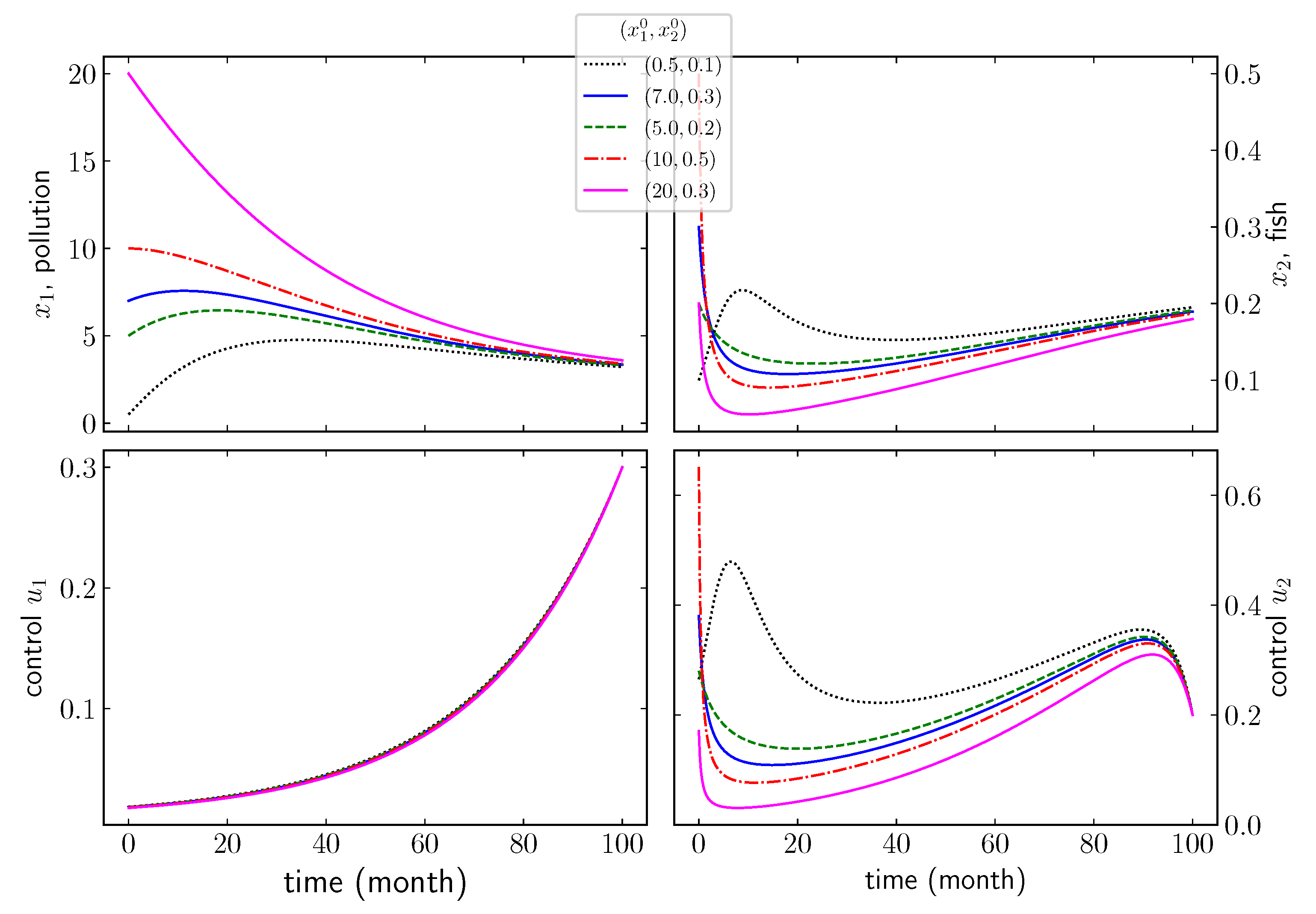
The control $u_{{}_2}$ is highly sensitive to the initial value of the state variables compared to the control $u_{{}_1}$, see Figure 2. When the pollution starts at a high level, the fish population decreases during the first year, before starting the monotonic growth. However, for low-level pollution, the fish population initially grows before becoming damped by the players’ activities.

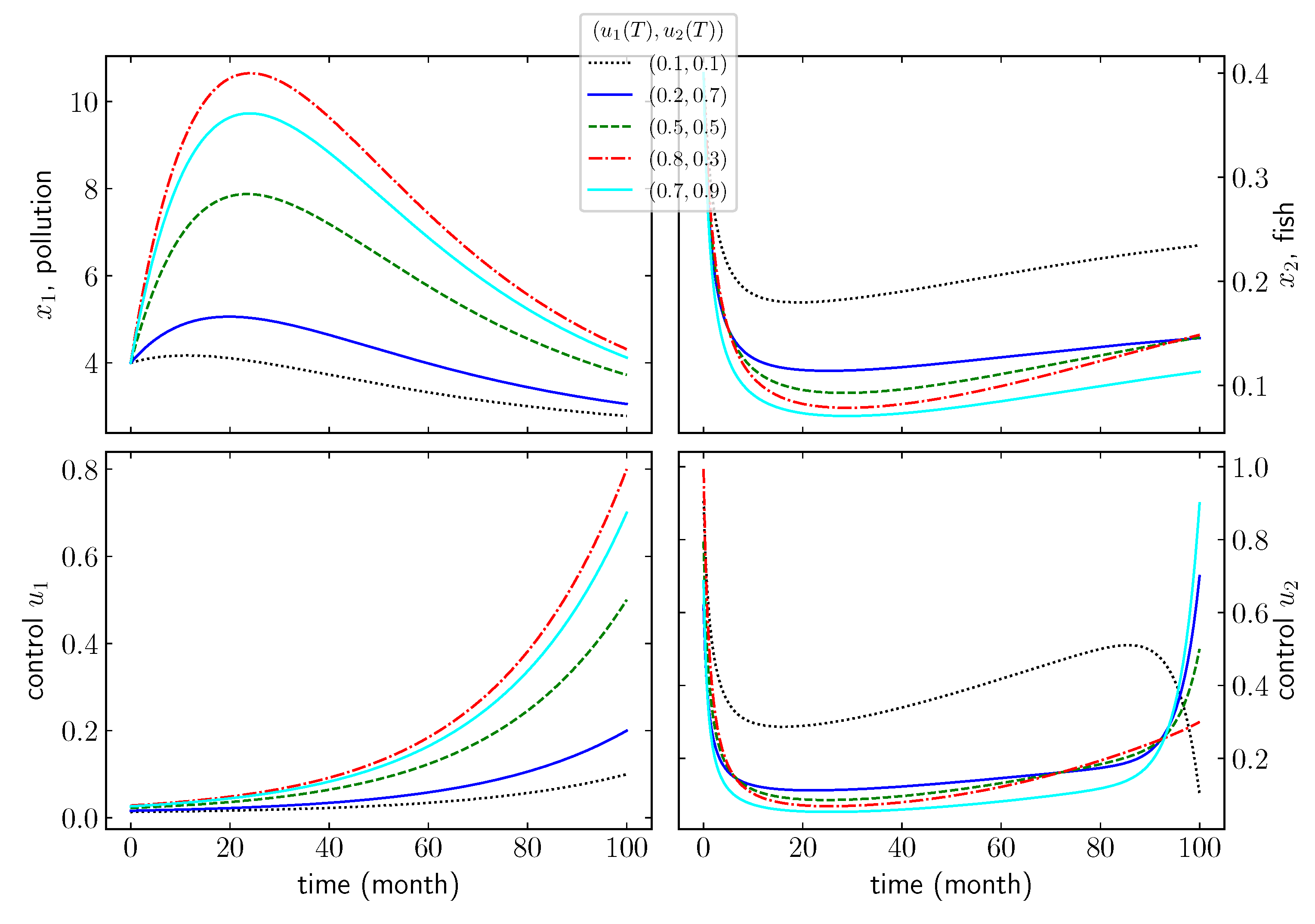
By combining one fixed initial condition state with several terminal conditions for the control variables (see Figure 3), we observe that the pollution control variable $u_{{}_1}$ is a consistently increasing function. Moreover, we see that the pollution state grows with the terminal condition value of $u_{{}_1}$ for the first two years but decays after. Subsequently, the fish population takes advantage of this and starts a slight growth.

The non-cooperative outcome, presented in the current Section 4, is a dynamic Nash equilibrium between the fishing industry and the other industries involved in pollution. From the perspective of global performance, this non-cooperative differs from the fully cooperative. The idea here can help to cooperate and enforce cooperation between the parties.

5. Cooperative Strategies and Biodiversity

Now, we examine the cooperative optimization of the players’ profits. Instead of a direct bilateral collaboration between the players, the cooperation is coordinated by a third entity such as state representations or international organizations. In practice, countries and international regulations have designed different rules, including incentive mechanisms, taxation, control, risk, and surveillance. Below, we examine one particular disincentive mechanism for pollution control.

5.1. The Optimal Strategy

To preserve the fish population, the political entity defines the global payoff and, as strategy designer, is in charge of setting the values of the parameters in the players’ utility and the cost functions. The global payoff function is given by:

$$\begin{array}{c}\hfill J(x_0,\widehat{u})={\int }_0^T\left({\widehat{\alpha }}_{{}_1}{\widehat{u}}_{{}_1}\left(t\right)-{\widehat{\gamma }}_{{}_1}\frac{{\widehat{u}}_{{}_1}^2\left(t\right)}{2}+{\widehat{\alpha }}_{{}_2}{x}_{{}_2}\left(t\right){\widehat{u}}_{{}_2}\left(t\right)-{\widehat{\gamma }}_{{}_2}(1-x_{{}_2}\left(t\right))\frac{{\widehat{u}}_{{}_2}^2\left(t\right)}{2}\right)dt+g\left(x\left(T\right)\right).\end{array}$$

The utilities of the players are similar to the non-cooperative case ones but the cost function changes particularly for the fishermen. Although the primary objective of the cooperation is biodiversity preservation, the fishermen take substantial benefits from it. This is because the efficient running of the fisheries’ activities is intrinsically associated with the level of fish population. Later on, the profit for the polluters will be discussed. We are then concerned with the optimal control problem:

$$\begin{array}{c}\hfill \left(\mathcal{P}\right)\left\{\begin{array}{c}{\displaystyle w\left(t\right)=\underset{\widehat{u}\left(t\right)}{sup}J(x_0,\widehat{u}),}\hfill \\ {\displaystyle \mathrm{subject} \mathrm{to} \left(1\right).}\hfill \end{array}\right.\end{array}$$

The pseudo-Hamiltonian is:

$$\begin{array}{c}\hfill H(t,x,({\widehat{q}}_{{}_1},{\widehat{q}}_{{}_2}),\widehat{u})=({\widehat{q}}_{{}_1},{\widehat{q}}_{{}_2})·f(x,\widehat{u})+{\widehat{\alpha }}_{{}_1}{\widehat{u}}_{{}_1}\left(t\right)-{\widehat{\gamma }}_{{}_1}\frac{{\widehat{u}}_{{}_1}^2\left(t\right)}{2}+{\widehat{\alpha }}_{{}_2}{x}_{{}_2}\left(t\right){\widehat{u}}_{{}_2}\left(t\right)-{\widehat{\gamma }}_{{}_2}(1-x_{{}_2}\left(t\right))\frac{{\widehat{u}}_{{}_2}^2\left(t\right)}{2}.\end{array}$$

A maximizer of H with respect to the control $\widehat{u}=({\widehat{u}}_{{}_1},{\widehat{u}}_{{}_2})$ provides an open-loop optimal control ${\widehat{u}}^{*}$ associated with the adjoint state $({\widehat{q}}_{{}_1},{\widehat{q}}_{{}_2})$ given by: ${\dot{\widehat{q}}}_{{}_1}\left(t\right)=-\frac{\partial H}{\partial x_{{}_1}}$ and ${\dot{\widehat{q}}}_{{}_2}\left(t\right)=-\frac{\partial H}{\partial x_{{}_2}}$. We find that:

$$\begin{array}{c}\hfill \left\{\begin{array}{c}{\displaystyle {\dot{\widehat{q}}}_{{}_1}\left(t\right)=-{\widehat{q}}_{{}_1}\left(-c+\frac{2b{x}_{{}_1}}{{(x_{{}_1}^2+1)}^2}\right)-r{\widehat{q}}_{{}_2}\left(t\right)x_{{}_2}^2\left(t\right)\frac{K^{\prime }\left(x_{{}_1}\right)}{K^2\left(x_{{}_1}\right)},}\hfill \\ {\displaystyle {\dot{\widehat{q}}}_{{}_2}\left(t\right)=-{\widehat{q}}_{{}_2}\left(r-\frac{2r{x}_{{}_2}}{K\left(x_{{}_1}\right)}-2x_{{}_2}{\widehat{u}}_{{}_2}\right)-{\widehat{\alpha }}_{{}_2}{\widehat{u}}_{{}_2}-{\widehat{\gamma }}_{{}_2}\frac{{\widehat{u}}_{{}_2}^2}{2}}\hfill \end{array}\right.\end{array}$$

(19)

running to the terminal condition: $\left({\widehat{q}}_{{}_1}\left(T\right),{\widehat{q}}_{{}_2}\left(T\right)\right)=\left({\partial }_{x_{{}_1}}g\left(x\left(T\right)\right),{\partial }_{x_{{}_2}}g\left(x\left(T\right)\right)\right)$.

The pseudo-Hamiltonian H is concave in the control variable $\widehat{u}$; the first-order optimality condition is then sufficient as in the non-cooperative scenario. The optimal control $\widehat{u}=({\widehat{u}}_{{}_1},{\widehat{u}}_{{}_2})$ of the cooperative strategy is given by $\frac{\partial H}{\partial {\widehat{u}}_{{}_1}}=0$ and $\frac{\partial H}{\partial {\widehat{u}}_{{}_2}}=0$, which are written in detail as follows:

$$\begin{array}{c}\hfill {\widehat{q}}_{{}_1}\left(t\right)+{\widehat{\alpha }}_{{}_1}-{\widehat{\gamma }}_{{}_1}{\widehat{u}}_{{}_1}\left(t\right)=0\mathrm{and}{\widehat{\gamma }}_{{}_2}(1-x_{{}_2}\left(t\right)){\widehat{u}}_{{}_2}\left(t\right)=-{\widehat{q}}_{{}_2}\left(t\right)x_{{}_2}^2\left(t\right)+{\widehat{\alpha }}_{{}_2}{x}_{{}_2}\left(t\right).\end{array}$$

By using the co-state Equation (19) in the differential form of the above optimality equations, we obtain:

$$\begin{array}{c}\hfill \left\{\begin{array}{c}{\displaystyle {\widehat{\gamma }}_{{}_1}{\dot{\widehat{u}}}_{{}_1}\left(t\right)=-({\widehat{\gamma }}_{{}_1}{\widehat{u}}_{{}_1}\left(t\right)-{\widehat{\alpha }}_{{}_1})\left(-c+\frac{2b{x}_{{}_1}\left(t\right)}{{(x_{{}_1}^2\left(t\right)+1)}^2}\right)}\hfill \\ {\displaystyle +r\left({\widehat{\gamma }}_{{}_2}(1-x_{{}_2}\left(t\right)){\widehat{u}}_{{}_2}\left(t\right)-{\widehat{\alpha }}_{{}_2}{x}_{{}_2}\left(t\right)\right)x_{{}_2}^2\left(t\right)\frac{K^{\prime }\left(x_{{}_1}\right)}{K^2\left(x_{{}_1}\right)},}\hfill \\ \\ {\displaystyle {\dot{\widehat{u}}}_{{}_2}\left(t\right)=\frac{2r-x_{{}_2}^2\left(t\right){\widehat{u}}_{{}_2}\left(t\right)}{2(1-x_{{}_2}\left(t\right))}{\widehat{u}}_{{}_2}\left(t\right)-\frac{r{x}_{{}_2}^2\left(t\right)}{K\left(x_{{}_1}\left(t\right)\right)\left(1-x_{{}_2}\left(t\right)\right)}\left({\widehat{\alpha }}_{{}_2}/{\widehat{\gamma }}_{{}_2}+{\widehat{u}}_{{}_2}\left(t\right)\right),}\hfill \end{array}\right.\end{array}$$

(20)

which has to be equipped with the terminal conditions:

$$\begin{array}{c}\hfill {\widehat{\gamma }}_{{}_1}{\widehat{u}}_{{}_1}\left(T\right)={\partial }_{x_{{}_1}}g\left(x\left(T\right)\right)+{\widehat{\alpha }}_{{}_1}\mathrm{and}{\widehat{\gamma }}_{{}_2}(1-x_{{}_2}\left(t\right)){\widehat{u}}_{{}_2}\left(T\right)={\widehat{\alpha }}_{{}_2}{x}_{{}_2}\left(T\right)-{\partial }_{x_{{}_2}}g\left(x\left(T\right)\right)\left(t\right)x_{{}_2}^2\left(T\right).\end{array}$$

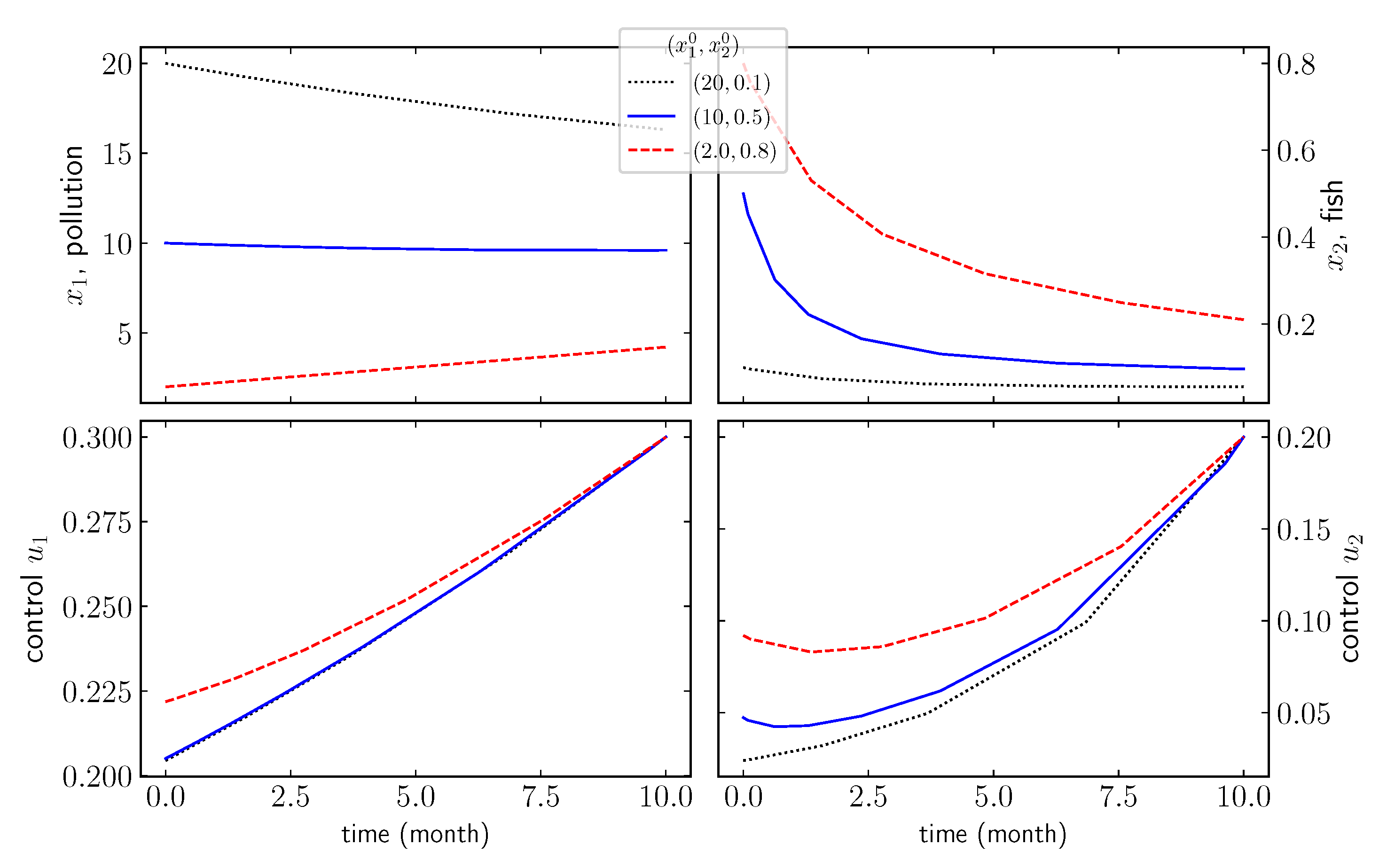
In Figure 4, we illustrate the optimal dynamics of the state and control variables for a period of 10 months. Here, the shooting method convergence is hard to achieve; therefore, an optimization algorithm is deployed in advance in order to approximate the initial conditions $u_{{}_i}\left(0\right)$ associated with the terminal conditions $u_{{}_i}\left(T\right)$. The main observation is that the dynamics of the state and control variables behave quite similarly to the non-cooperative regime. In the next section, we investigate the benefits of the cooperative regime.

5.2. Taxation: Incentive Design

In this section, we investigate sufficient beneficial conditions for the implementation of the cooperative strategy. In order to achieve efficiency of the cooperative strategy, the decision-makers set, implement, and control the policy for the players, such that their rewards when cooperating are greater than the total sum of the value functions in the non-cooperative scenario. From the dynamics programming approach of Bellman in control theory, the value functions $v_{{}_1}$ and $v_{{}_2}$ obey the followings Hamilton–Jacobi–Bellman equations:

$$\begin{array}{c}\hfill \left\{\begin{array}{c}{\displaystyle \frac{\partial v_{{}_1}}{\partial t}-\left(c{x}_{{}_1}-\frac{b{x}_{{}_1}^2}{x_{{}_1}^2+1}\right)\frac{\partial v_{{}_1}}{\partial x_{{}_1}}+{\mathcal{H}}_1\left(x_{{}_1},v_{{}_1},\frac{\partial v_{{}_1}}{\partial x_{{}_1}}\right)=0,}\hfill \\ \\ {\displaystyle \frac{\partial v_{{}_2}}{\partial t}+r{x}_{{}_2}\left(1-\frac{x_{{}_2}}{K\left(x_{{}_1}\right)}\right)\frac{\partial v_{{}_2}}{\partial x_{{}_2}}+{\mathcal{H}}_2\left(x_{{}_2},v_{{}_2},\frac{\partial v_{{}_2}}{\partial x_{{}_2}}\right)=0,}\hfill \\ \\ {\displaystyle v_{{}_1}(x_{{}_1},T)=g_{{}_1}\left(x_{{}_1}\right),}\hfill \\ \\ {\displaystyle v_{{}_2}(x_{{}_2},T)=g_{{}_2}\left(x_{{}_2}\right),}\hfill \end{array}\right.\end{array}$$

(21)

where:

$$\begin{array}{ccc}\hfill {\mathcal{H}}_1\left(x_{{}_1},v_{{}_1},\frac{\partial v_{{}_1}}{\partial x_{{}_1}}\right)& =& \underset{u_{{}_1}\in {\mathcal{A}}_1}{max}\left\{u_{{}_1}\frac{\partial v_{{}_1}}{\partial x_{{}_1}}+{\alpha }_{{}_1}{u}_{{}_1}-{\gamma }_{{}_1}\frac{u_{{}_1}^2}{2}\right\},\hfill \\ \hfill {\mathcal{H}}_2\left(x_{{}_2},v_{{}_2},\frac{\partial v_{{}_2}}{\partial x_{{}_2}}\right)& =& \underset{u_{{}_2}\in {\mathcal{A}}_2}{max}\left\{-x_{{}_2}^2{u}_{{}_2}\frac{\partial v_{{}_2}}{\partial x_{{}_2}}+{\alpha }_{{}_2}{x}_{{}_2}{u}_{{}_2}-{\gamma }_{{}_2}(1-x_{{}_2})\frac{u_{{}_2}^2}{2}\right\}.\hfill \end{array}$$

Indeed, the admissible control set ${\mathcal{A}}_{{}_i}$ is a compact bounded subset of $\mathbb{R}$, the component i of the drift function at (2) is Lipschitz continuous, and the running cost ${\mathcal{U}}_i-{\mathcal{C}}_i$ is bounded and continuous with respect to the control variable $u_{{}_i}$ for $i=1,2$. Therefore, according to the dynamics programming, the value function $v_{{}_i}$ defined in (13) is a continuous viscosity solution of:

$$\begin{array}{c}\hfill \frac{\partial v_{{}_i}(t,x_{{}_i})}{\partial t}+\underset{u_{{}_i}\in {\mathcal{A}}_i}{max}{H}_i\left(x,v_{{}_i},\frac{\partial v_{{}_i}}{\partial x_{{}_i}},u_{{}_i}\right)=0,\end{array}$$

(22)

where $H_i$, for $i=1,2$, is given in (13) and (14). Writing the pseudo-Hamiltonians $H_1$ and $H_1$ as:

$$\begin{array}{ccc}\hfill H_1& =& -\left(c{x}_{{}_1}-\frac{b{x}_{{}_1}^2}{x_{{}_1}^2+1}\right)\frac{\partial v_{{}_1}}{\partial x_{{}_1}}+\underset{u_{{}_1}\in {\mathcal{A}}_1}{max}\left\{u_{{}_1}\frac{\partial v_{{}_1}}{\partial x_{{}_1}}+{\alpha }_{{}_1}{u}_{{}_1}-{\gamma }_{{}_1}\frac{u_{{}_1}^2}{2}\right\},\hfill \\ \hfill H_2& =& r{x}_{{}_2}\left(1-\frac{x_{{}_2}}{K\left(x_{{}_1}\right)}\right)\frac{\partial v_{{}_2}}{\partial x_{{}_2}}+\underset{u_{{}_2}\in {\mathcal{A}}_2}{max}\left\{-x_{{}_2}^2{u}_{{}_2}\frac{\partial v_{{}_2}}{\partial x_{{}_2}}+{\alpha }_{{}_2}{x}_{{}_2}{u}_{{}_2}-{\gamma }_{{}_2}(1-x_{{}_2})\frac{u_{{}_2}^2}{2}\right\},\hfill \end{array}$$

we obtain the HJB equations in (21).

In the same sequel, the aggregated value function w, in the cooperative policy, exists (the admissible control set $\mathcal{A}={\mathcal{A}}_1\times {\mathcal{A}}_2$ is a compact bounded subset of ${\mathbb{R}}^2$, the drift function is Lipschitz continuous, and the aggregated running cost is continuous and bounded) and is governed by the following HJB equation:

$$\begin{array}{c}\hfill \left\{\begin{array}{c}{\displaystyle \frac{\partial w}{\partial t}-\left(c{x}_{{}_1}-\frac{b{x}_{{}_1}^2}{x_{{}_1}^2+1}\right)\frac{\partial w}{\partial x_{{}_1}}+r{x}_{{}_2}\left(1-\frac{x_{{}_2}}{K\left(x_{{}_1}\right)}\right)\frac{\partial w}{\partial x_{{}_2}}+\mathcal{H}(x,w,\nabla w)=0,}\hfill \\ \\ {\displaystyle w(x,T)=g\left(x\right),}\hfill \end{array}\right.\end{array}$$

(23)

where:

$$\begin{array}{ccc}& & \mathcal{H}(x,w,\nabla w)=\hfill \\ & & \underset{\widehat{u}\in \mathcal{A}}{max}\left\{{\widehat{u}}_{{}_1}\frac{\partial w}{\partial x_{{}_1}}+{\widehat{\alpha }}_{{}_1}{\widehat{u}}_{{}_1}\left(t\right)-{\widehat{\gamma }}_{{}_1}\frac{{\widehat{u}}_{{}_1}^2\left(t\right)}{2}-x_{{}_2}^2{\widehat{u}}_{{}_2}\frac{\partial w}{\partial x_{{}_2}}+{\widehat{\alpha }}_{{}_2}{x}_{{}_2}\left(t\right){\widehat{u}}_{{}_2}\left(t\right)-{\widehat{\gamma }}_{{}_2}(1-x_{{}_2}\left(t\right))\frac{{\widehat{u}}_{{}_2}^2\left(t\right)}{2}\right\}.\hfill \end{array}$$

To show the efficiency of the cooperation, under the aegis of legal authority, in terms of biodiversity preservation and without damping the players’ outcomes, one needs to quantify the value functions $v_{{}_1}$, $v_{{}_2}$, and w and perform a comparison analysis. However, the value functions are solutions of HJB partial differential equations that require the design of a high-order numerical method with a strong flux limiter—see [18,19]—to approximate $v_{{}_1}$, $v_{{}_2}$, and w. Next, we state a sufficient condition in the running cost definition to implement the cooperative regime that subsequently causes the players to accept the cooperative regime as the best.

Proposition 12.

Given the same circumstances in the non-cooperative and cooperative scenarios (same business growth rate, same level of pollution, and same approved fish stock to be harvested), the sufficient conditions for the players to cooperate, without trying to cheat, are:

$$\begin{array}{c}\hfill {\gamma }_i>{\widehat{\gamma }}_{i}fori=1,2.\end{array}$$

(24)

Proof. 

Players should accept and align with the cooperative regime if, and only if, the aggregated rewards are greater than the sum of what they earn, as business outcomes, in the non-cooperative case, i.e., $v_{{}_1}+v_{{}_2}\le w$. The business growth rate is given by the time variation of the value function: in the non-cooperative scenario, it is given by $\frac{\partial v_{{}_i}}{\partial t}$, while in the cooperative regime, we have the global growth rate $\frac{\partial w}{\partial t}$. The same business growth rate in both regimes means that $\frac{\partial w}{\partial t}=\frac{\partial v_{{}_1}}{\partial t}+\frac{\partial v_{{}_2}}{\partial t}$. Then, it remains to compare ${\mathcal{H}}_1+{\mathcal{H}}_2$ and $\mathcal{H}$ with the same level of pollution and same fish stock to be harvested.

The utility function of the fishermen ${\alpha }_{{}_2}{x}_{{}_2}{u}_{{}_2}$ in the non-cooperative regime and ${\widehat{\alpha }}_{{}_2}{x}_{{}_2}{\widehat{u}}_{{}_2}$ in the cooperation scenario should remain the same to avoid rough variations of the fish price that amplify the life cost for the population. Similarly, the gross gain of the polluters is basically given by the level of the residual chemicals and might depend also on the market state, but not on whether there is cooperation or not. This yields the condition ${\alpha }_{{}_1}={\widehat{\alpha }}_{{}_1}$ and the analysis is reduced to compare:

$$\begin{array}{c}\hfill \underset{u_{{}_1}\in {\mathcal{A}}_1}{max}\left\{u_{{}_1}\frac{\partial v_{{}_1}}{\partial x_{{}_1}}-{\gamma }_{{}_1}\frac{u_{{}_1}^2}{2}\right\}+\underset{u_{{}_2}\in {\mathcal{A}}_2}{max}\left\{-x_{{}_2}^2{u}_{{}_2}\frac{\partial v_{{}_2}}{\partial x_{{}_2}}-{\gamma }_{{}_2}(1-x_{{}_2})\frac{u_{{}_2}^2}{2}\right\}\end{array}$$

and

$$\begin{array}{c}\hfill \underset{\widehat{u}\in \mathcal{A}}{max}\left\{{\widehat{u}}_{{}_1}\frac{\partial w}{\partial x_{{}_1}}-{\widehat{\gamma }}_{{}_1}\frac{{\widehat{u}}_{{}_1}^2}{2}-x_{{}_2}^2{\widehat{u}}_{{}_2}\frac{\partial w}{\partial x_{{}_2}}-{\widehat{\gamma }}_{{}_2}(1-x_{{}_2})\frac{{\widehat{u}}_{{}_2}^2}{2}\right\}.\end{array}$$

However, the polluters expect better business growth with regard to the amount of generated residual chemicals when cooperating, i.e., $\frac{\partial v_{{}_1}}{\partial x_{{}_1}}\le \frac{\partial w}{\partial x_{{}_1}}$. Similarly, fishermen await a better growth of their business from the aggregated value function in terms of the fish stock $x_{{}_2}$. This means $\frac{\partial v_{{}_2}}{\partial x_{{}_2}}\le \frac{\partial w}{\partial x_{{}_2}}$. Therefore, we find that the sufficient condition $v_{{}_1}+v_{{}_2}\le w$ can be formulated as follows:

$$\begin{array}{c}\hfill \underset{u_{{}_1}\in {\mathcal{A}}_1}{max}\left\{-{\gamma }_{{}_1}\frac{u_{{}_1}^2}{2}\right\}+\underset{u_{{}_2}\in {\mathcal{A}}_2}{max}\left\{-{\gamma }_{{}_2}(1-x_{{}_2})\frac{u_{{}_2}^2}{2}\right\}\le \underset{\widehat{u}\in \mathcal{A}}{max}\left\{-{\widehat{\gamma }}_{{}_1}\frac{{\widehat{u}}_{{}_1}^2}{2}-{\widehat{\gamma }}_{{}_2}(1-x_{{}_2})\frac{{\widehat{u}}_{{}_2}^2}{2}\right\}.\end{array}$$

(25)

It is obvious that (25) holds for $-{\gamma }_1<-{\widehat{\gamma }}_1$ and $-{\gamma }_2<-{\widehat{\gamma }}_2$, which means that ${\gamma }_1>{\widehat{\gamma }}_1$ and ${\gamma }_2>{\widehat{\gamma }}_2$. □

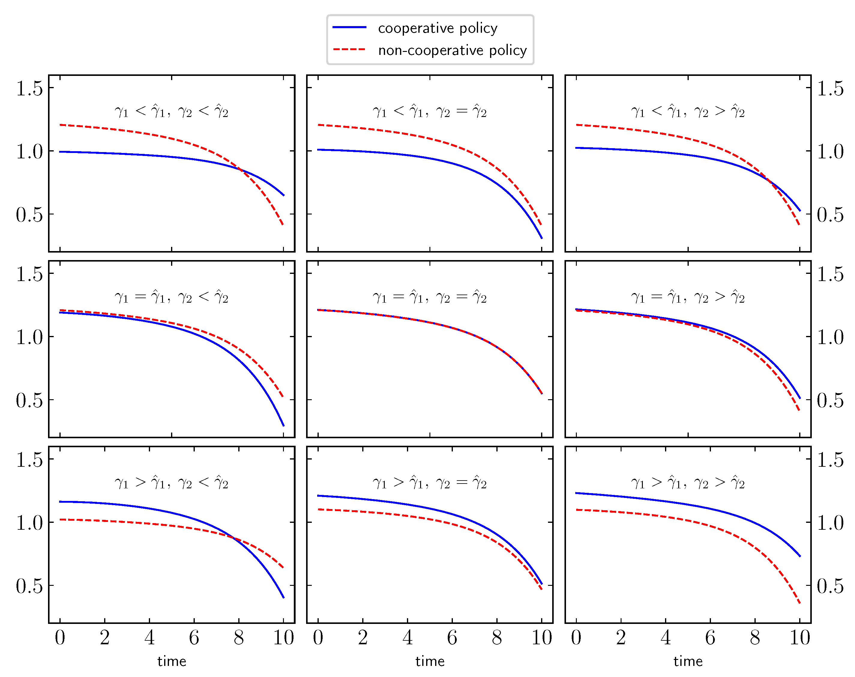
The plotted running costs in Figure 5 are obtained by taking the arithmetic mean over 10 runs for each case. Our comparison analysis matches well with the theoretical statement, which claims that (24) is a sufficient but not a necessary condition to align all the players with the cooperative policy. In fact, we can see clearly that the plot ${\gamma }_i>{\widehat{\gamma }}_i$ for $i=1,2$ gives a consistent advantage to the cooperation.

6. Conclusions

We introduced a system of differential equations describing the impact of the pollution from industrial and agricultural companies in the fish population in watercourses subject to fishery activities. The stability analysis highlights the necessity of controlling the pollution input to preserve the fish population and, subsequently, the fishery industries. The non-cooperative optimal control is not the worse-case scenario for fishermen as both classes of players incorporate the fish preservation into the payoff definition. However, the cooperative strategy under the authority of a third entity seems to be more advantageous for fish preservation. Implementing an incentive taxation approach for setting the parameters’ values helps the third entity as it means that the players should not try to cheat.

One central aspect missed in this work is as follows: normally, it is not the pollution caused by an individual farmer or one single industry that harms people’s health but it is the aggregate effect of all polluting entities. This is the starting point of our future work to introduce a mean-field approach [20,21] with the distribution of polluters and also to quantify the pollution generated by fishermen.

References

- Ganguly, S. Leather processing industries generate effluents causing environmental and water pollution: An Asian perspective. J. Ind. Lea. Tech. Assoc. LXII 2012, 12, 1133–1137. [Google Scholar]
- Ganguly, S. Water pollution from various sources and human infringements: An editorial. Ind. J. Sci. Res. Tech. 2013, 1, 54–55. [Google Scholar]
- Sharma, P. Weblog on Keeping Word Environment Safer and Greener Oil Spilsâ Adverse Effects on Marine Environmental Bio-System and Control Measure. Environment. 2008. Available online: saferenvironment.wordpress.com (accessed on 18 August 2021).
- Crunkilton, R.L.; Duchrow, R.M. Impact of a massive crude oil spill on the invertebrate fauna of a missouri ozark stream. Environ. Pollut. 1990, 63, 13–31. [Google Scholar] [CrossRef]
- Khatua, A.; Jana, A.; Kar, T.K. A fuzzy rule-based model to assess the effects of global warming, pollution and harvesting on the production of Hilsa fishes. Ecol. Inform. 2020, 57, 101070. [Google Scholar] [CrossRef]
- Auger, P.; Lett, C.; Moussaoui, A.; Pioch, S. Optimal number of sites in artificial pelagic multi-site fisheries. Can. J. Fish. Aquat. Sci. 2010, 67, 296–303. [Google Scholar] [CrossRef]
- Ly, S.; Auger, P.; Balde, M. A bioeconomic model of a multi-site fishery with nonlinear demand function: Number of sites optimizing the total catch. Acta Biotheor. 2014, 62, 371–384. [Google Scholar] [CrossRef] [PubMed]
- Brochier, T.; Auger, P.; Thiao, D.; Bah, A.; Ly, S.; Nguyen-Huu, T.; Brehmer, P. Can over-exploited fisheries recover by self-organization? reallocation of fishing effort as an emergent form of governance. Mar. Policy 2018, 95, 46–56. [Google Scholar] [CrossRef]
- Bergl, H.; Burlakov, E.; Pedersen, P.A.; Wyller, J. Aquaculture, pollution and fishery dynamics of marine industrial interactions. Ecol. Complex. 2020, 43, 100853. [Google Scholar] [CrossRef]
- Tahvonen, O. On the dynamics of renewable resource harvesting and pollution control. Environ. Resour. Econ. 1991, 1, 97–117. [Google Scholar]
- Pochai, N.; Tangmanee, V.; Crane, L.J.; Miller, J.J.H. A mathematical model of water pollution control using the finite element method. Proc. Appl. Math. Mech 2006, 6, 755–756. [Google Scholar] [CrossRef]
- Carpenter, S.R.; Ludwig, D.; Brock, W.A. Management of eutrophication for lakes subject to potentially irreversible change. Ecol. Appl. 1999, 9, 751–771. [Google Scholar] [CrossRef]
- Palomares, M.; Froese, R.; Derrick, B.; Meeuwig, J.; Nöel, S.-L.; Tsui, G.; Woroniak, J.; Zeller, D.; Pauly, D. Fishery biomass trends of exploited fish populations in marine eco-regions, climatic zones and ocean basins. Estuarine Coast. Shelf Sci. 2020, 243, 106896. [Google Scholar] [CrossRef]
- Kossioris, G.; Plexousakis, M.; Xepapadeas, A.; de Zeeuw, A.; Mäler, K.-G. Feedback Nash equilibria for non-linear differential games in pollution control. J. Econ. Dyn. Control. 2008, 32, 1312–1331. [Google Scholar] [CrossRef] [Green Version]
- Dia, B.M.; Diagne, M.L.; Goudiaby, M.S. Optimal control of invasive species with economic benefits: Application to the Typha proliferation. Nat. Resour. Model. 2020, 33, e12268. [Google Scholar] [CrossRef]
- Jones, J.H. Notes on R0. Department of Anthropological Sciences; Stanford University: Stanford, CA, USA, 2007; Volume 323. [Google Scholar]
- Pontryagin, L.; Boltyanskii, V.; Gamkrelidze, R.; Mishchenko, E. The Mathematical Theory of Optimal Processes; A Pergamon Press Book; The Macmillan Co.: New York, NY, USA, 1964. [Google Scholar]
- Carlini, E.; Ferretti, R.; Russo, G. A weighted essentially nonoscillatory, large time-step scheme for Hamilton-Jacobi equations. SIAM J. Sci. Comput. 2005, 27, 1071–1091. [Google Scholar] [CrossRef] [Green Version]
- Liu, X.D.; Osher, S.; Chan, T. Weighted essentially non-oscillatory schemes. J. Comput. Phys. 1994, 115, 200–212. [Google Scholar] [CrossRef] [Green Version]
- Bauso, D.; Dia, B.M.; Djehiche, B.; Tembine, H.; Tempone, R. Mean-field games for marriage. PLoS ONE 2014, 9, e94933. [Google Scholar] [CrossRef] [PubMed] [Green Version]
- Bauso, D.; Tembine, H.; Başar, T. Robust mean field games. Dyn. Games Appl. 2016, 6, 277–303. [Google Scholar] [CrossRef]
Figure 1.
Phase field of the uncontrolled dynamics for (top left), (right) and (bottom left).
Figure 2.
Dynamic of the controlled model with : one terminal condition for the control combined with different starting states .
Figure 3.
Dynamic of the controlled model with starting at combined with several terminal conditions for the control .
Figure 4.
Dynamics of the state and control variables in the cooperative scenario for the terminal condition for the control combined with different starting states .
Figure 5.
Comparison of the aggregated running cost in the cooperative regime (blue line) and the sum of the two running costs in the non-cooperative regime (red dashed line) starting at (). Pollution control and fish population control after months are and , respectively, and and .
Publisher’s Note: MDPI stays neutral with regard to jurisdictional claims in published maps and institutional affiliations. |
© 2021 by the authors. Licensee MDPI, Basel, Switzerland. This article is an open access article distributed under the terms and conditions of the Creative Commons Attribution (CC BY) license (https://creativecommons.org/licenses/by/4.0/).
Share and Cite
MDPI and ACS Style
Goudiaby, M.S.; Dia, B.M.; Diagne, M.L.; Tembine, H. Cooperative Game for Fish Harvesting and Pollution Control. Games 2021, 12, 65. https://0-doi-org.brum.beds.ac.uk/10.3390/g12030065
AMA Style
Goudiaby MS, Dia BM, Diagne ML, Tembine H. Cooperative Game for Fish Harvesting and Pollution Control. Games. 2021; 12(3):65. https://0-doi-org.brum.beds.ac.uk/10.3390/g12030065
Chicago/Turabian StyleGoudiaby, Mouhamadou Samsidy, Ben Mansour Dia, Mamadou L. Diagne, and Hamidou Tembine. 2021. "Cooperative Game for Fish Harvesting and Pollution Control" Games 12, no. 3: 65. https://0-doi-org.brum.beds.ac.uk/10.3390/g12030065
Note that from the first issue of 2016, this journal uses article numbers instead of page numbers. See further details here.