
CEO Bias and Product Substitutability in Oligopoly Games


Department of Economics, Oregon State University, Corvallis, OR 97331, USA
*
Author to whom correspondence should be addressed.
Games 2022, 13(2), 28; https://0-doi-org.brum.beds.ac.uk/10.3390/g13020028
Submission received: 1 March 2022
/
Revised: 21 March 2022
/
Accepted: 25 March 2022
/
Published: 31 March 2022
(This article belongs to the Topic Game Theory and Applications)
Abstract
:We investigate why a firm might purposefully hire a chief executive officer (CEO) who under- or over-estimates the degree of substitutability between competing products. This counterintuitive result arises in imperfect competition because CEO bias can affect rival behavior and the intensity of competition. We lay out the conditions under which it is profitable for owners to hire biased managers. Our work shows that a universal policy that effectively eliminates such biases need not improve social welfare.
1. Introduction
A large and growing body of evidence reveals that chief executive officers are not always perfectly rational. In fact, CEOs can be subject to a variety of behavioral biases1. Empirical evidence has shown that CEOs often systematically misestimate economic conditions. We provide the first theoretical framework to explain why owners may prefer to hire CEOs who make systematic measurement errors.
One example of this type of mismeasurement is firms’ frequent miscalculation of the effectiveness of marketing. The pioneering work by Blake et al. [8] and the follow-up study by Rao and Simonov [9] address the case of internet advertising. Blake et al. estimate that the return to advertising spending for eBay was negative 63%. Although eBay dropped brand advertising as a result of the study, in Rao and Simonov only 11% of firms changed their advertising spending in response to information regarding the ineffectiveness of internet marketing. Rao and Simonov suggest that this counterintuitive result may derive from a principal–agent problem, in that the goals of management diverge from the goals of the firm. Additionally, Rao and Simonov indicate that management may be unaware of the best method to accurately estimate demand and cost conditions. In that case, corporate decisions rely on potentially erroneous information.
In this paper, we claim that it can be rational for owners to hire CEOs who persistently make biased estimates of demand conditions. This result can occur because CEO behavior can evoke changes in rival strategies under imperfect competition. We include these strategic effects in our analysis and focus on product substitutability, which has not yet been studied in this setting.
Our work contributes to the burgeoning literature on behavioral economics as applied to management bias. CEO overconfidence, for example, has received considerable attention in the literature. Early work documenting that many CEOs are overconfident has motivated theoretical analysis designed to explain why boards of directors (owners) might choose to hire CEOs with biased levels of confidence2. We contribute to the behavioral literature by being the first to investigate a model with CEOs who may make biased estimates of demand.
In our model, firms compete by producing homogeneous or differentiated products, and consumers determine the degree of product substitutability. For example, consumers decide on the extent to which a wooden pencil is a substitute for a mechanical pencil. The degree of substitutability is unknown to the firm and, therefore, must be estimated by CEOs (or their research staff). This estimate ultimately affects firm behavior and the degree of competition among rivals.
Our model shows that whether it is profit-maximizing for an owner to hire a biased CEO depends on the mode of competition. In a non-strategic setting (i.e., perfect competition and monopoly), it is always optimal for owners to hire unbiased CEOs. In a strategic setting, however, CEO bias may be able to profitably shape competitor behavior. In particular, we find that the decision to hire a CEO who overestimates or underestimates product substitutability depends on whether firms compete in output or price in the product market.
In the strategic setting, we consider models with two competitors and three modes of competition. These include the traditional models of Cournot, where both firms compete in output, and Bertrand, where both firms compete in price. We also consider the Cournot–Bertrand model (Bylka and Komar [19]), where one firm competes in output and the other competes in price. The Cournot–Bertrand model has been used to analyze issues in a variety of fields, including international economics, public economics, and industrial organization. Further, hybrid quantity–price behavior is observed in real markets (e.g., among producers of alcoholic beverages, small car retailers, and foreign vs. domestic producers of manufactured goods)3. Given the strategic asymmetry of the Cournot–Bertrand model, it may generate results that differ from those in the traditional models.
In the next section, we develop a model to address these issues. Firms compete in a two-stage game. In the first stage, owners hire CEOs who may or may not be biased. In the second stage, firms (CEOs) compete in either output or price in the product market. We investigate the non-strategic settings of perfect competition and monopoly, but our primary focus is on imperfect competition where two firms compete in output or price. In Section 3, we summarize the results and the welfare implications. We find that it is optimal for owners to hire an unbiased CEO in non-strategic settings, while it pays to hire a biased CEO in strategic settings. The direction of bias depends on the mode of competition and on the effect of one CEO’s bias on its competitor’s best-reply function. The conclusion follows in Section 4.
2. CEO Estimation Bias in Classic Oligopoly Games
Consider a market where strategic decisions depend upon the extent of product differentiation. Because consumers determine the degree of substitutability, it is unknown and must be estimated by firms. Our main goal is to determine whether it is optimal for owners to intentionally hire CEOs who base corporate decisions on biased estimates of product substitutability. We briefly discuss this problem in monopoly and competitive settings, but our focus is on an imperfectly competitive market where two firms produce substitute goods4.
Firms 1 and 2 play a two-stage game. In our notation, subscript i identifies one of the firms and subscript j identifies that firm’s competitor. In stage I, each owner maximizes profit () by deciding whether to search for and hire a CEO who may make a biased estimate of the degree of substitutability between competing products. A CEO’s type is identified by parameter , which indexes the extent of estimation bias. In our specification, CEOi is unbiased when . Overestimation of product substitutability occurs when and underestimation occurs when . It is assumed that there is a pool of potential CEOs with varying degrees of bias. In stage II, owners delegate corporate decisions to CEOs. At this stage, CEOs compete in the product market where they make output () or price () decisions, depending on the mode of competition: Cournot, Bertrand, and Cournot–Bertrand. Each CEO maximizes expected profit, based on their type and the mode of competition. At each stage, decisions are made simultaneously, and economic agents have perfect and complete information.
Each game is assumed to be well-behaved. Costs are sufficiently low to assure firm participation. Profit functions are strictly concave and twice-continuously differentiable, such that the first- and second-order conditions of profit maximization are met for all choice variables. Each game has a unique and stable equilibrium and the “typical” math structure5. We also assume that each game has a unique Stackelberg equilibrium (d’Aspremont and Gérard-Varet [23]).
To determine whether it would pay owners to hire biased CEOs, we use backwards induction to identify the subgame perfect Nash equilibrium (SPNE). The forces that shape these decisions are determined by owner foresight regarding the stage II behavior of CEOs concerning the choice variable = or . When evaluated at the simple Nash equilibrium of and where there is no bias (), hiring a biased CEO is optimal when deviation from unbiasedness raises profit. More formally, the total effect on firm i’s profit from deviation of for the owner is:
The first set of terms on the right-hand side of the equality is the own effect on firm i’s profit that results from a marginal increase in . It equals zero, given profit maximization . The second set of terms identifies the strategic effect that occurs because of the resulting change in the action of firm j. If Equation (1) is zero, then it pays to hire an unbiased CEO. If it is positive (negative), however, it is optimal to hire a CEO who overestimates (underestimates) product substitutability.
Equation (1) demonstrates that market structure can influence an owner’s decision. In the absence of strategic effects, as in perfect competition and monopoly markets, the strategic effect is zero and owners hire unbiased CEOs. In an imperfectly competitive setting, however, the strategic effect need not be zero and its sign depends on the mode of competition and the extent to which the CEO’s bias affects rival behavior.
The strategic effect contains two components. The first is the indirect effect , which identifies how changes in response to the change in . This reflects a movement along firm j’s best-reply function, which derives from firm j’s first-order condition of profit maximization. The second is the direct effect , which occurs when the change in directly affects the best-reply function (or the first-order condition) of firm j6.
When discussing the various models below, we consider general and specific functional forms. The specific cases build from the duopoly framework found in Dixit [24] and Singh and Vives [25] that is commonly used in the overconfidence literature. In this model, product demand derives from a representative consumer who has a quadratic and concave utility function. The resulting inverse demand functions are:
where and . Given symmetry, firm i’s demand can be written as . For simplicity, let , where parameter d is an index of product differentiation or substitutability. Products are homogeneous or perfect substitutes when and are unrelated when (i.e., each firm is a monopolist). Thus, the degree of substitutability increases as and decreases as . Given that the Nash equilibrium in the product market is identical to the competitive outcome in the Bertrand case for homogeneous goods, we assume that products are imperfect substitutes, . A firm’s cost of production, , is normalized to zero to simplify the discussion.
In this specification, the presence of estimation bias is modeled as follows. Let the true value of . However, CEOi believes that and expects demand to equal . For the unbiased CEO, and expected demand equals true demand. When the CEO underestimates product substitutability (i.e., , CEOi believes that products i and j are more differentiated or less substitutable than is true in reality. In other words, the CEO unrealistically believes that firm j is a softer or more distant competitor. This induces the CEO to increase the output/price toward the simple monopoly outcome, assuming no direct effect 7. We see, however, that this need not be true when there is also a direct effect. We investigate the motivation for hiring a biased CEO in each mode of competition.
2.1. Estimation Bias in a Cournot Game
We first consider Cournot competition in the output market, where firms optimize by simultaneously choosing quantities. For firm i, the owner’s goal is to maximize true profit: . Once hired, the CEO of firm i maximizes expected profit, , which depends on the degree of CEO bias. Expected profit equals true profit only when .
To analyze the case where owners consider hiring biased CEOs, we use backwards induction to obtain the SPNE. In stage II, where CEOs optimize over output, Nash equilibrium values are and . In stage I, firm i’s profit depends upon first-stage choices, and , and the anticipated actions in the second period, and . That is, . This model implies the following results:
Proposition 1.
Consider this two-stage game with Cournot competition in stage II and where both firms have the option of hiring a biased CEO [, ] in stage I.
- A.
- If a change in has no direct effect on in the neighborhood of the simple Cournot outcome where , then both firms hire CEOs who underestimate the degree of product substitutability ().
- B.
- If a change in directly effects by shifting firm j’s best-reply function, then the sign of CEO estimation bias is indeterminate.
Proof.
Given that underestimation of the degree of product substitutability induces CEOi to increase production, in the neighborhood of the simple Cournot outcome where . As a result, and both firms hire CEOs who underestimate the degree of product substitutability ().
In this case, the sign of is indeterminant without knowing the sign and the relative magnitude of the direct effect . □
When corresponds to output, Equation (1) becomes:
With profit maximization, ; therefore, the first set of terms on the right-hand side of the equality equals 0. Given that products are substitutes, . Because firm j’s best-reply function has a negative slope with Cournot competition, .
- In the absence of a direct effect of on , the following is true:
- B.
- With a direct effect:
To further illustrate, we consider the linear model of Dixit [24] and Singh and Vives [25], as discussed above. This specification provides an example of Part A of Proposition 1, because a change in has no direct effect on firm j’s best-reply function. In stage II, CEOs simultaneously maximize expected profit with respect to output. Recall that when biased, CEOi believes that and, therefore, expects profit to be . In this symmetric game, firm i’s first-order condition of profit maximization is . Firm i’s best-reply function (BRi) is:
Notice that there are no direct effects in this model, as does not depend on . In terms of , firm i’s best-reply function can be written as8:
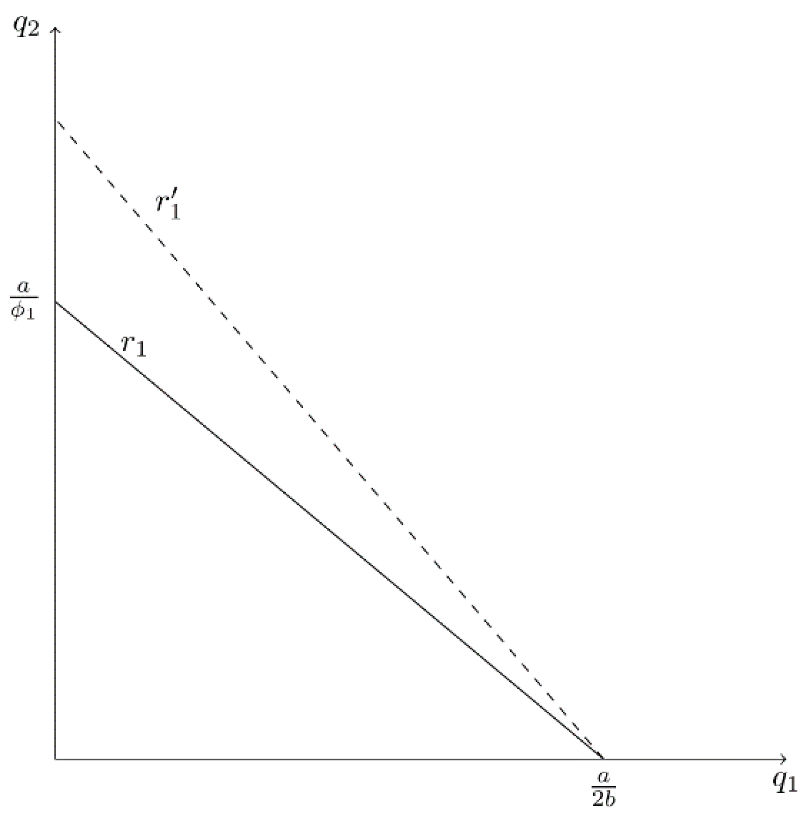
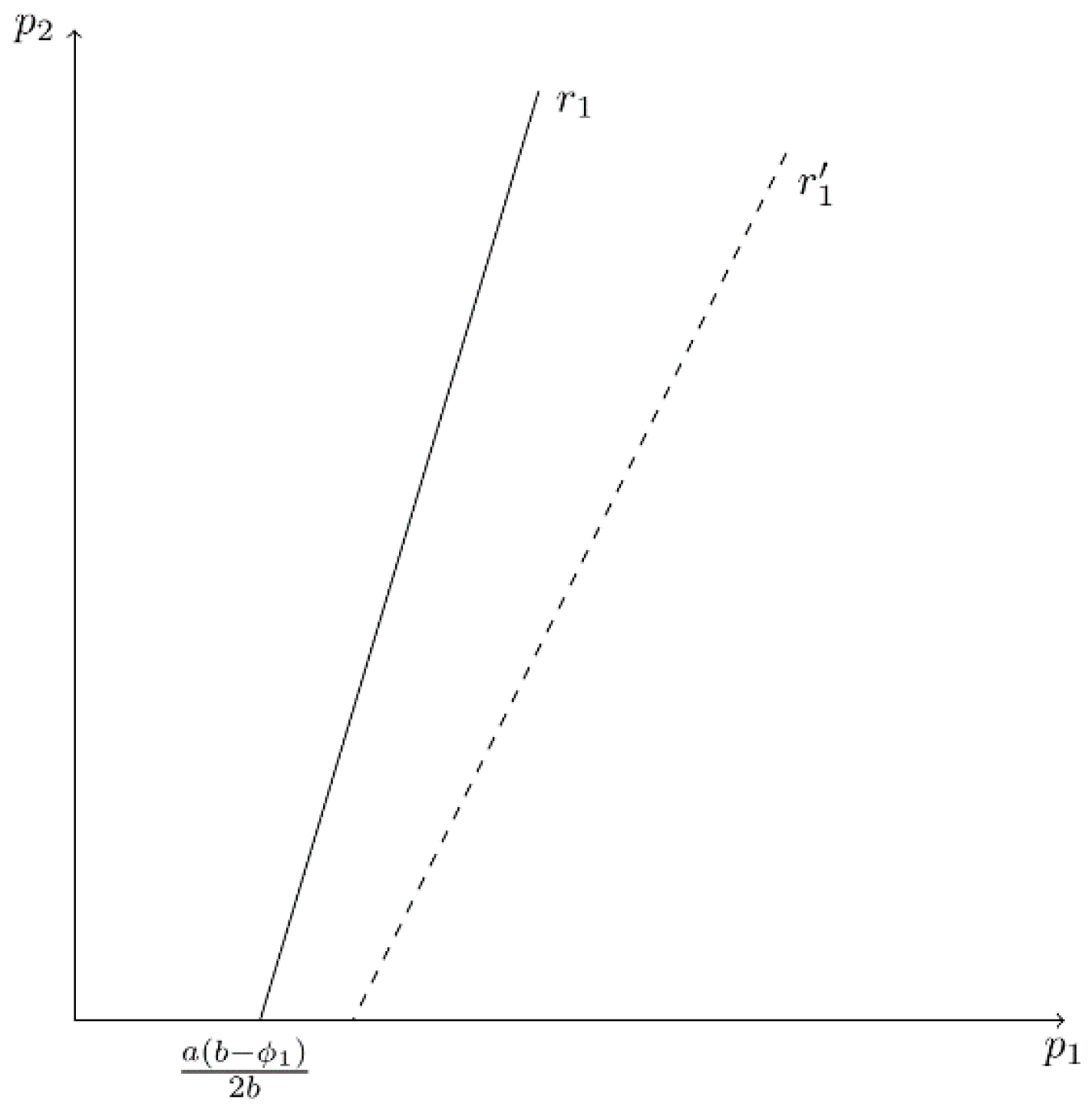
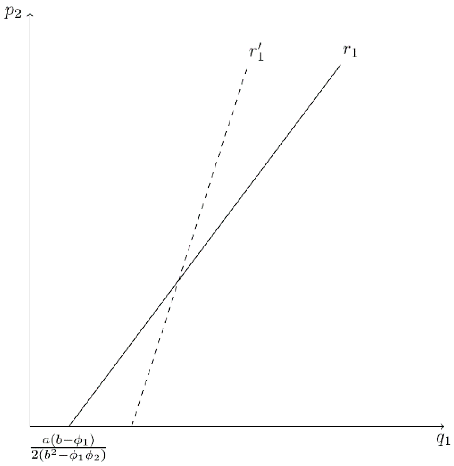
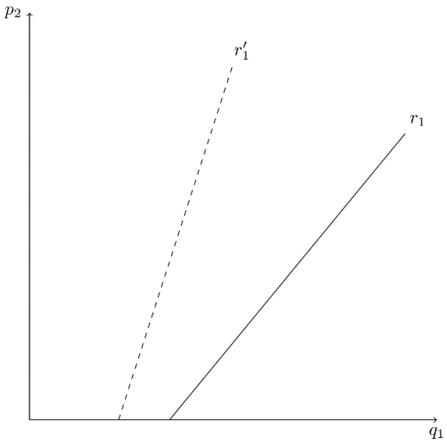
Figure 1 provides a graph of firm 1’s best-reply curve (r1), with on the horizontal axis and on the vertical axis. Note that the -intercept equals the simple monopoly output level, , which is optimal when . Furthermore, if the CEO of firm 1, CEO1, underestimates the degree of product substitutability to a greater extent (i.e., decreases), r1 becomes steeper and rotates around the -intercept (from r1 to in Figure 1). That is, firm 1 is willing to produce more output for a given . In stage II, the Nash equilibrium (NE) level of output is:
In stage I, owners simultaneously choose to maximize true profit, given the anticipated output choices of CEOs in stage II, which are identified as and . Thus, owner i anticipates profit to be:
Firm i’s first-order condition of profit maximization is:
In this model, when evaluated at the simple Nash equilibrium where . Thus, the optimal value of is less than 1 (i.e., each owner has an incentive to hire a CEO who underestimates ).
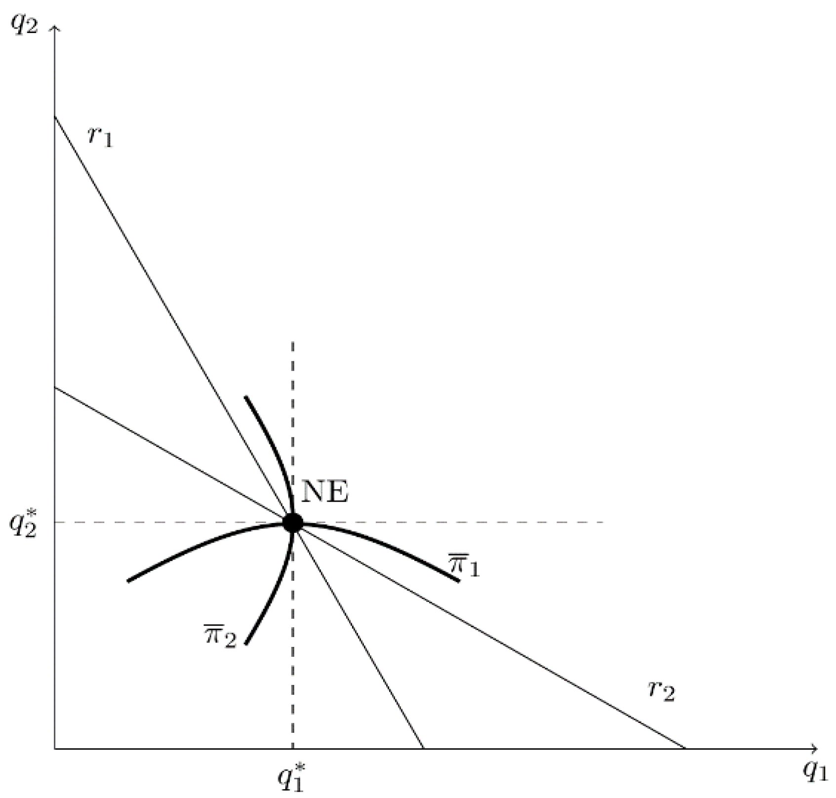
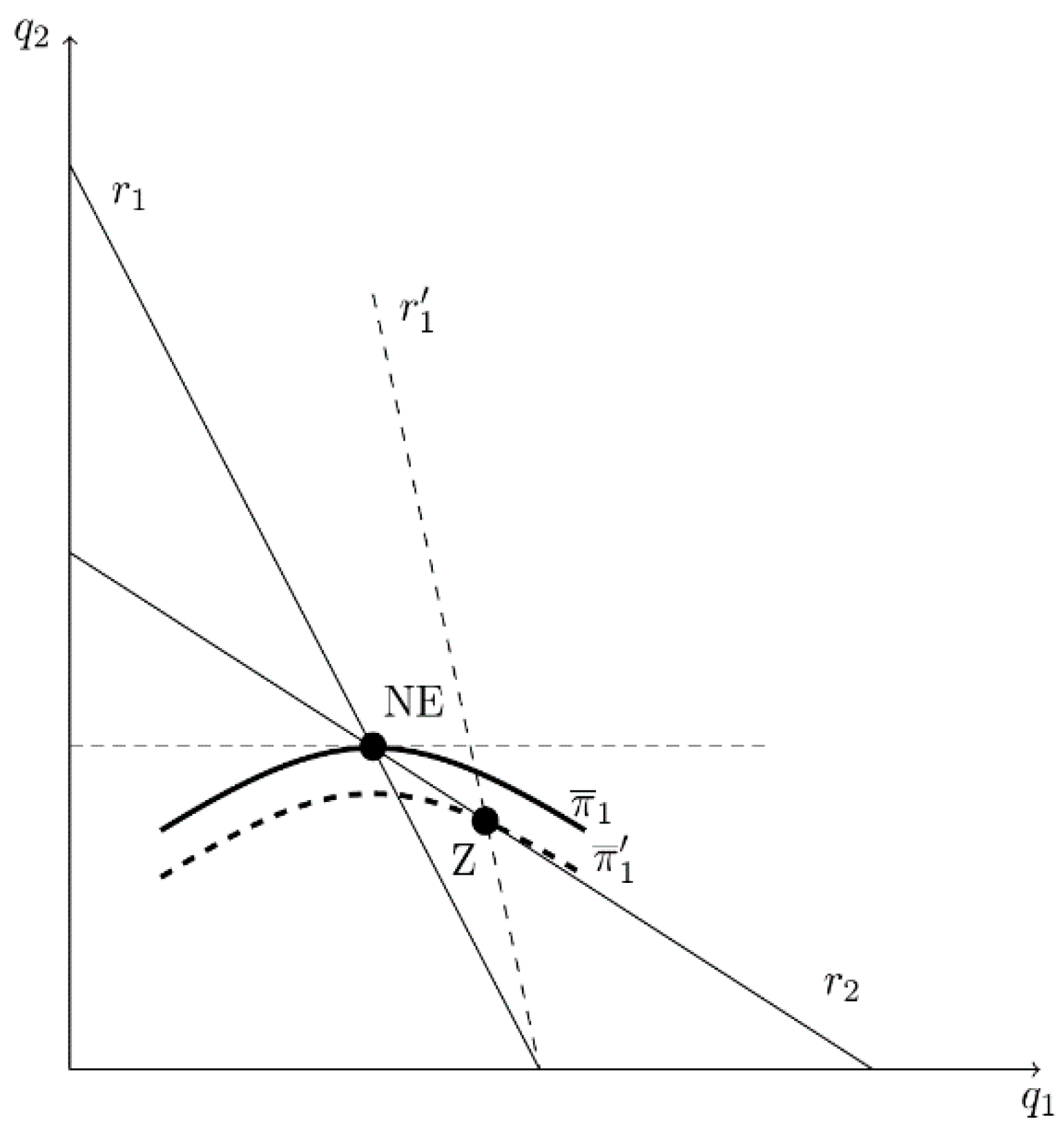
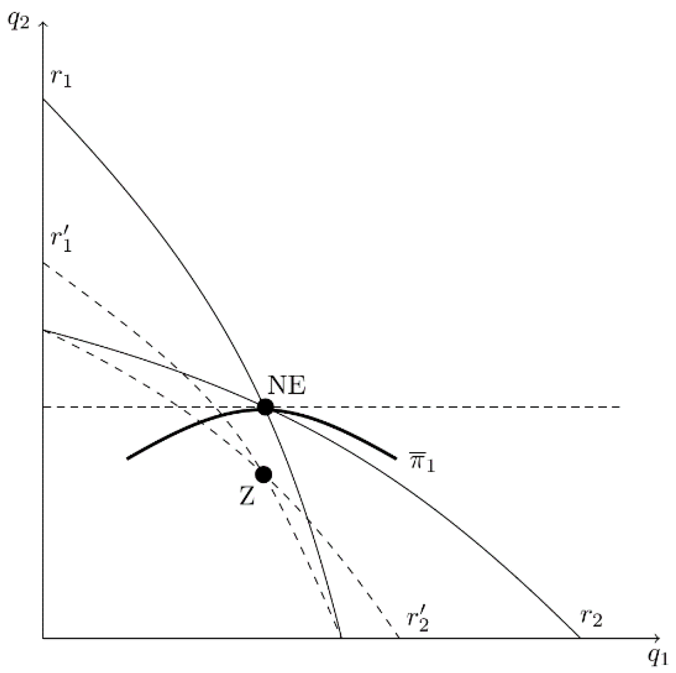
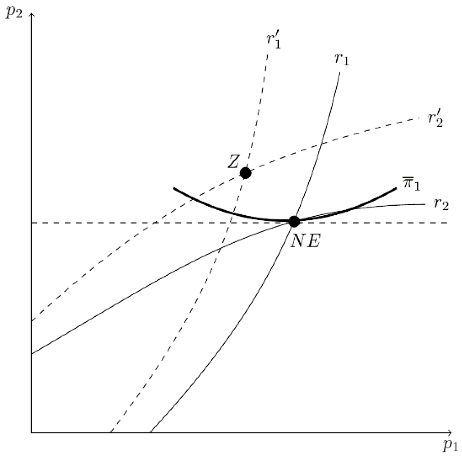
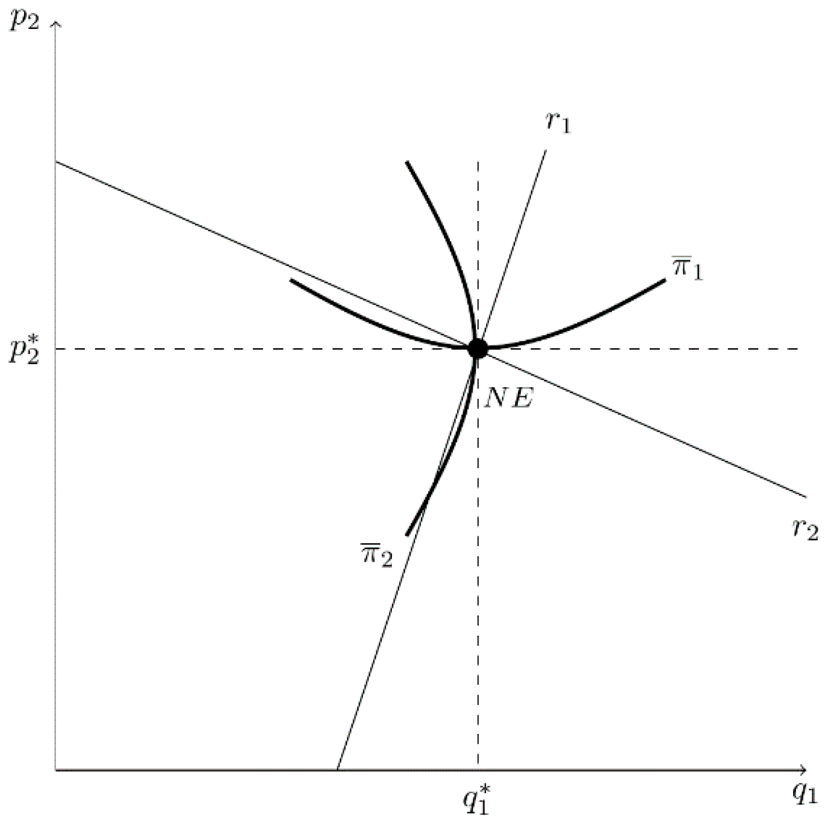
The intuition behind this result can be seen from the following Figures. Figure 2 identifies each firm’s best-reply curve, labeled and , and the simple Cournot (NE) outcome when there is no bias (). Firm i’s iso-profit curve () is concave to its own () axis, and an iso-profit curve that is closer to the firm’s own axis signifies higher profit. By definition of a best-reply function, at NE the slope of the tangent line to firm 1’s iso-profit curve is horizontal and the slope of the tangent to firm 2’s iso-profit curve is vertical. A marginal decrease in (underestimation of product substitutability) causes firm 1’s best reply to become steeper. As illustrated in Figure 3, rotates away from the origin and moves the equilibrium down firm 2’s best-reply curve toward point Z, the Stackelberg-type equilibrium. By underestimating the degree of substitutability between products, firm 2’s optimal output level increases9. This enables Firm 1 to reach a lower iso-profit curve, , representing higher profit. In other words, in this strategic setting, a marginal decrease in induces firm 2 to produce less output, which benefits firm 1. The same incentive applies to firm 2. Therefore, each owner has an incentive to hire a CEO who underestimates strategic effects. This is consistent with Part A of Proposition 1, because a change in has no effect on firm j’s best-reply curve.
When both owners simultaneously optimize over , SPNE values are listed in Table 1. It shows that it is optimal for owners to hire CEOs who underestimate strategic effects (. The table also includes the simple Cournot, cartel, and competitive outcomes in the absence of bias10. Note that the SPNE price is lower than the cartel and simple Cournot prices but exceeds the competitive price.
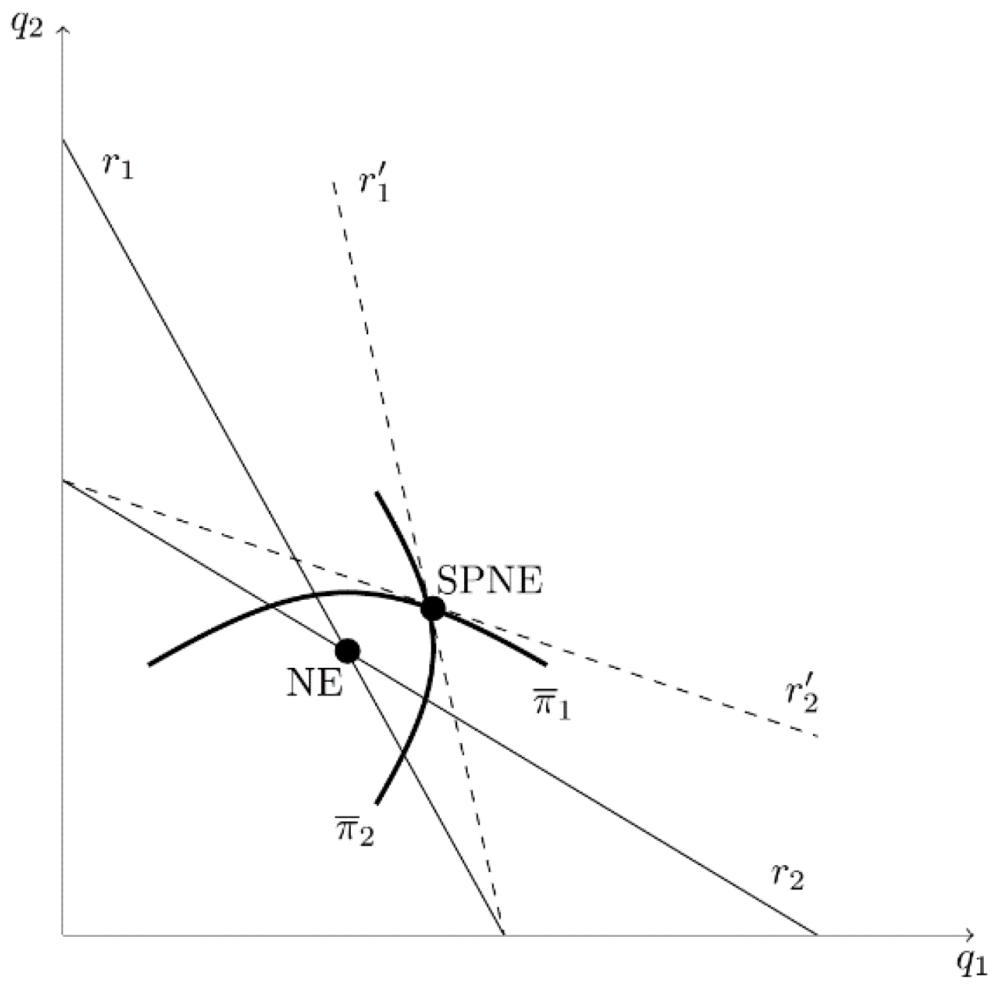
Figure 4 provides a graphical depiction of the SPNE, where NE identifies the simple Cournot outcome. When owners have the option of hiring biased CEOs in stage I, each owner chooses to maximize profit given the best reply of its competitor. Each firm hires a CEO who underestimates strategic effects, which rotates each firm’s best-reply function away from the origin. The SPNE is reached when these conditions simultaneously hold for both owners, which occurs when firm i’s iso-profit curve is tangent to firm j’s best-reply curve at SPNE in Figure 4. The reduction in below 1 leads to greater production and lower profits for both firms. Thus, the SPNE is superior to the simple Cournot and cartel outcomes from society’s perspective.
The intuition of Part B of Proposition 1 is apparent for a non-linear example where a change in causes both r1 and r2 to shift. Suppose that an increase in causes both r1 and r2 to rotate toward the origin, as illustrated in Figure 5. This means that the overestimation of product substitutability by CEO1 causes firm 2 to behave less aggressively (i.e., firm 2 produces less output for a given ). If this causes the new equilibrium point Z to lie below as illustrated in Figure 5, then and it would benefit the owner of firm 1 to hire a CEO who overestimates product substitutability (. Alternatively, if point Z is on , then it would pay the owner to hire an unbiased CEO (. Finally, if point Z is above , then it would pay the owner to hire a CEO who underestimates product substitutability (. A similar argument applies to firm 2, making it clear that the sign of the estimation bias is indeterminate.
2.2. Strategic Bias in a Bertrand Game
We use the same approach to investigate the Bertrand-type game. In this model, demand and profit equations depend on choice variables, and . Firm i’s true profit function is . CEOi’s price decision is based on expected profit, , which depends on the degree of CEO bias.
To analyze an owner’s decision to hire a biased CEO, we use backwards induction to identify the characteristics of the SPNE. In stage II, the Nash equilibrium prices are and . In stage I, firm i’s profit depends upon first-stage choices, and , and the anticipated actions in the second period, such that . In this model, the results are:
Proposition 2.
Consider this two-stage game with Bertrand competition in stage II and where both firms have the option of hiring a biased CEO [, ] in stage I.
- A.
- If a change in has no direct effect on in the neighborhood of the simple Bertrand outcome where , then both firms hire CEOs who underestimate the degree of product substitutability ().
- B.
- If a change in directly affects by shifting firm j’s best-reply function, then the sign of CEO estimation bias is indeterminate.
Proof.
Given that the underestimation of the degree of product substitutability induces CEOi to raise the price, in the neighborhood of the simple Bertrand outcome where . As a result, and both firms hire CEOs who underestimate the degree of product substitutability ().
In this case, the sign of is indeterminant without knowing the sign and relative magnitude of the direct effect . □
When corresponds to price, Equation (1) becomes:
With profit maximization, ; therefore, the first set of terms on the right-hand side of the equality equals 0. Given that products are substitutes, . Because firm j’s best-reply function has a positive slope with Bertrand competition, .
- In the absence of a direct effect of on , the following is true:
- B.
- With a direct effect:
To illustrate, we continue to use the linear model described above. As in the Cournot case, it provides an example that is consistent with Part A of Proposition 2, because a change in has no effect on firm j’s best-reply function. Firms face the same inverse demand system as before. In the Bertrand game, demand functions are obtained by inverting the inverse demand functions, Equations (2) and (3), for and . The true demand functions are:
With the potential for bias, which occurs when CEOi believes that , CEOs expect demand functions to be:
Solving the stage II problem first, CEOs simultaneously maximize expected profit with respect to price, where CEOi expects profit to be . Given symmetry and the first-order condition of profit maximization, the best-reply function for firm i in terms of is:
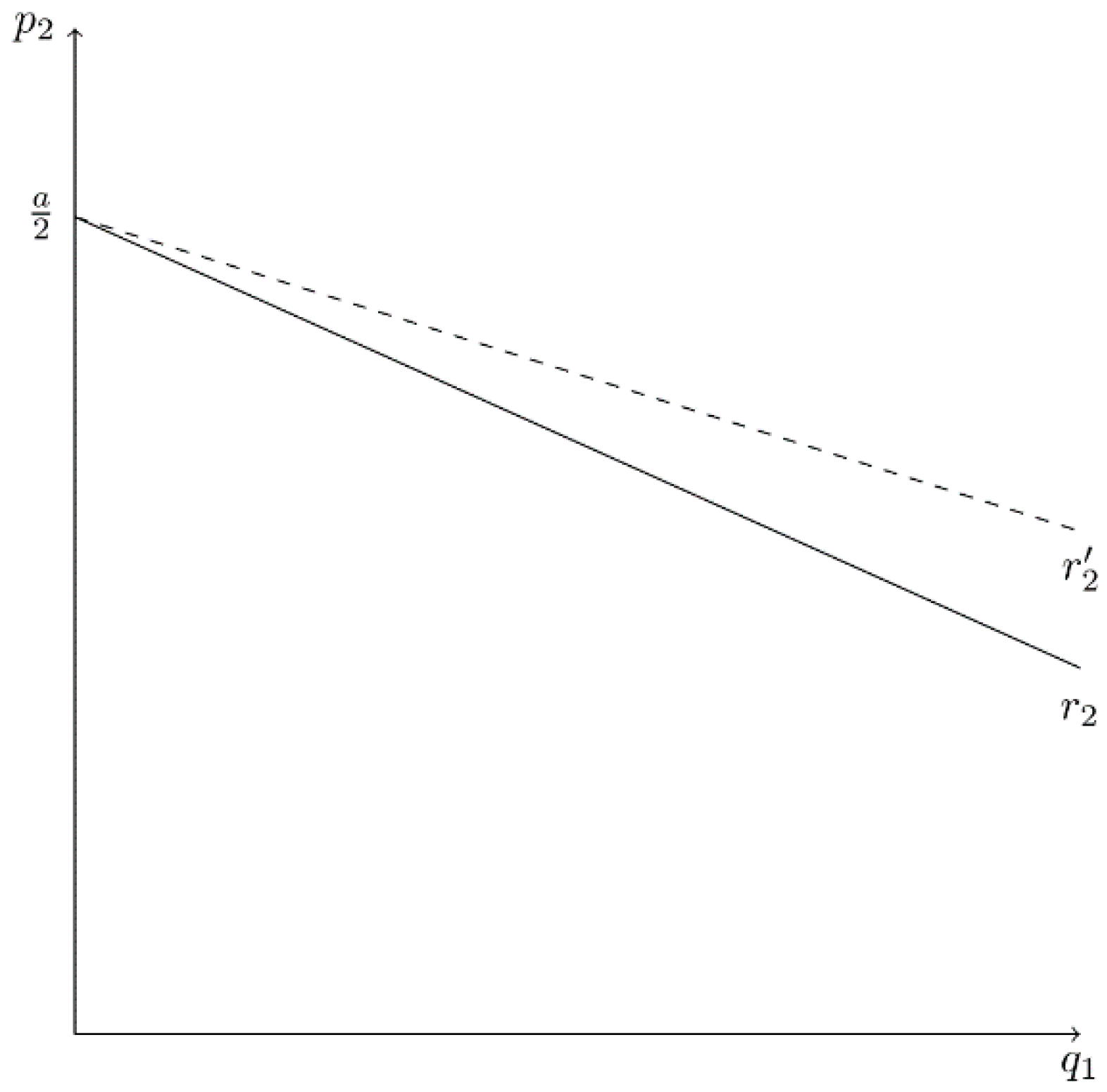
Figure 6 provides a graph of firm 1’s best-reply function, with on the horizontal axis and on the vertical axis. In the Bertrand case, the best-reply function has a positive slope and r1 does not depend on the value of . As decreases (i.e., CEO1 underestimates product substitutability), r1 becomes flatter and the -intercept increases. In the stage II subgame, firm i’s NE price is:
Figure 7 depicts best-reply curves and the simple Nash (Bertrand) equilibrium assuming no estimation bias (). In this case, each firm’s iso-profit curve is convex to its own axis and exhibits greater profit for iso-profit curves that are further from its own axis.
In stage I, owners simultaneously choose to maximize true profit, given the anticipated equilibrium prices in stage II, and . Thus, owner i anticipates profit to be:
The first-order condition of profit maximization is:
As in the Cournot case, when evaluated at the simple Bertrand equilibrium where . Thus, the optimal value of is less than 1.
When the owners of both firms consider hiring biased CEOs, SPNE values are listed in Table 2. It demonstrates that it is optimal for owners to hire CEOs who underestimate product substitutability (. The table also includes the simple Bertrand (NE) outcome. (The simple cartel and competitive outcomes are the same as in Table 1.) In this model, the SPNE price exceeds the simple Bertrand price but falls short of the cartel price.
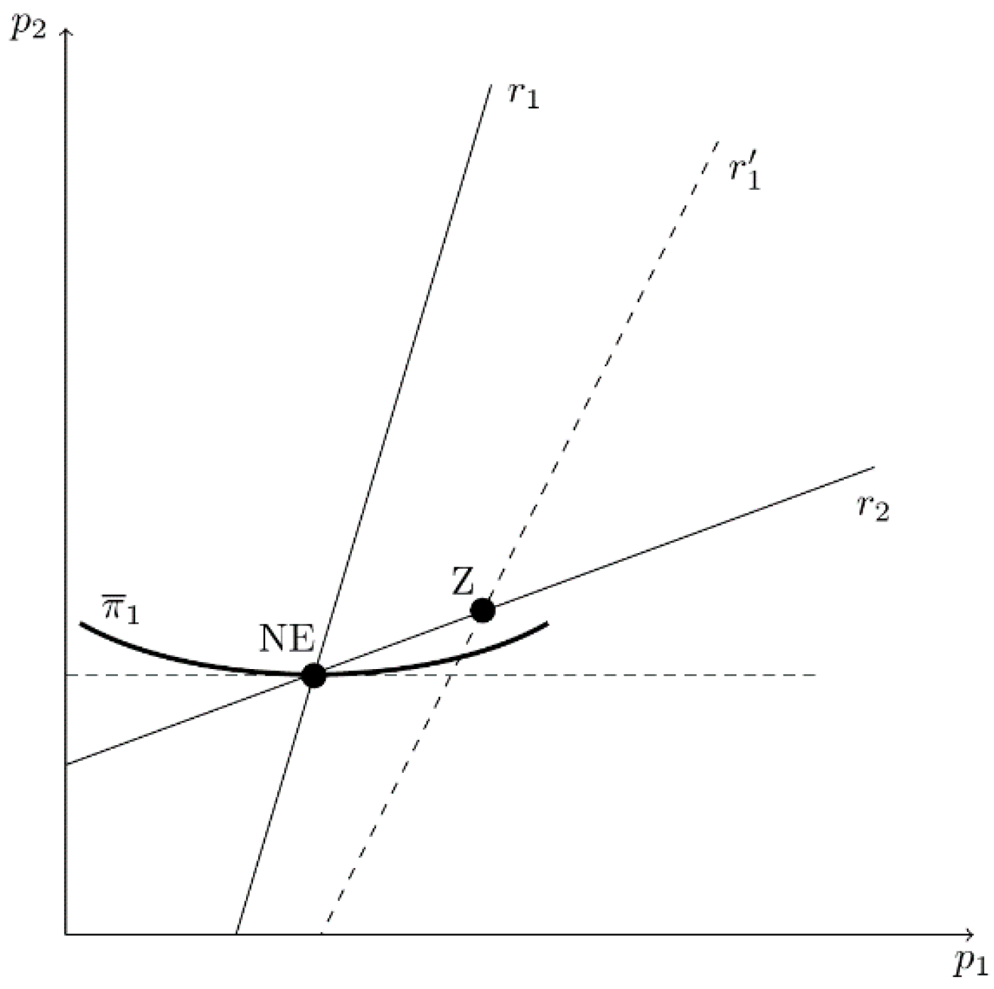
Figure 8 provides intuition for this result. It shows the best-reply curves ( and ), firm 1’s iso-profit curve, and the simple Bertrand equilibrium (NE). A marginal decrease in causes firm 1’s best reply to shift right from to . In this case, CEO1 believes that products 1 and 2 are less substitutable than is actually true, causing the firm’s optimal price to be greater for a given . By underestimating product substitutability, price competition is reduced and firm 1 earns greater profit as the equilibrium moves to a point such as Z11. In other words, a marginal decrease in induces firm 2 to charge a higher price, which benefits firm 1. The same argument applies to firm 2. Thus, each owner has an incentive to hire a CEO who underestimates product substitutability, a result that is consistent with Part A of Proposition 2.
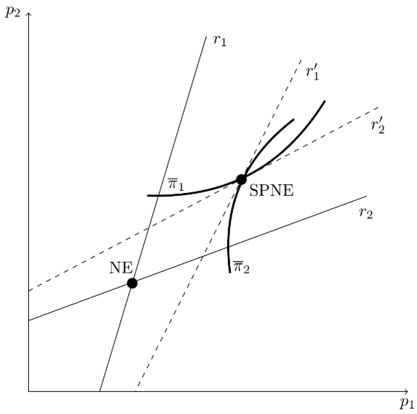
Figure 9 identifies the NE without bias and the SPNE. With the potential for bias, each owner chooses to maximize profit given the best reply of its competitor. As described in Figure 9, the SPNE is reached when each owner hires a CEO who underestimates product substitutability to the point where firm i’s iso-profit curve is tangent to firm j’s best-reply curve. In this two-stage game, each firm’s optimal is less than 1, a bias that leads to higher prices and profits for both firms (i.e., each firm’s iso-profit curve is further away from its own axis).
Figure 10 provides intuition for Part B of Proposition 2. In this example, a change in causes both r1 and r2 to shift. If an increase in causes both and to shift up so that the new equilibrium point Z lies below , then and it would benefit the owner of firm 1 to hire a CEO who overestimates product substitutability (. If point Z is on , then it would pay the owner to hire an unbiased CEO. Finally, if point Z is above , then it would pay the owner to hire a CEO who underestimates product substitutability. A similar argument applies to firm 2, making it clear that the sign of the estimation bias is indeterminate.
2.3. Strategic Bias in a Cournot–Bertrand Game
In this section, we assume Cournot–Bertrand competition in the product market. For concreteness, let firm 1 compete in output and firm 2 compete in price. With this mode of competition, demand and profit equations depend upon choice variables, and . Firm i’s true profit is , while CEOi bases decisions on expected profit: . Given the strategic asymmetry between firms, firm 1’s best-reply function has a positive slope and firm 2’s best-reply function has a negative slope, even when firms face the same cost and inverse demand functions.
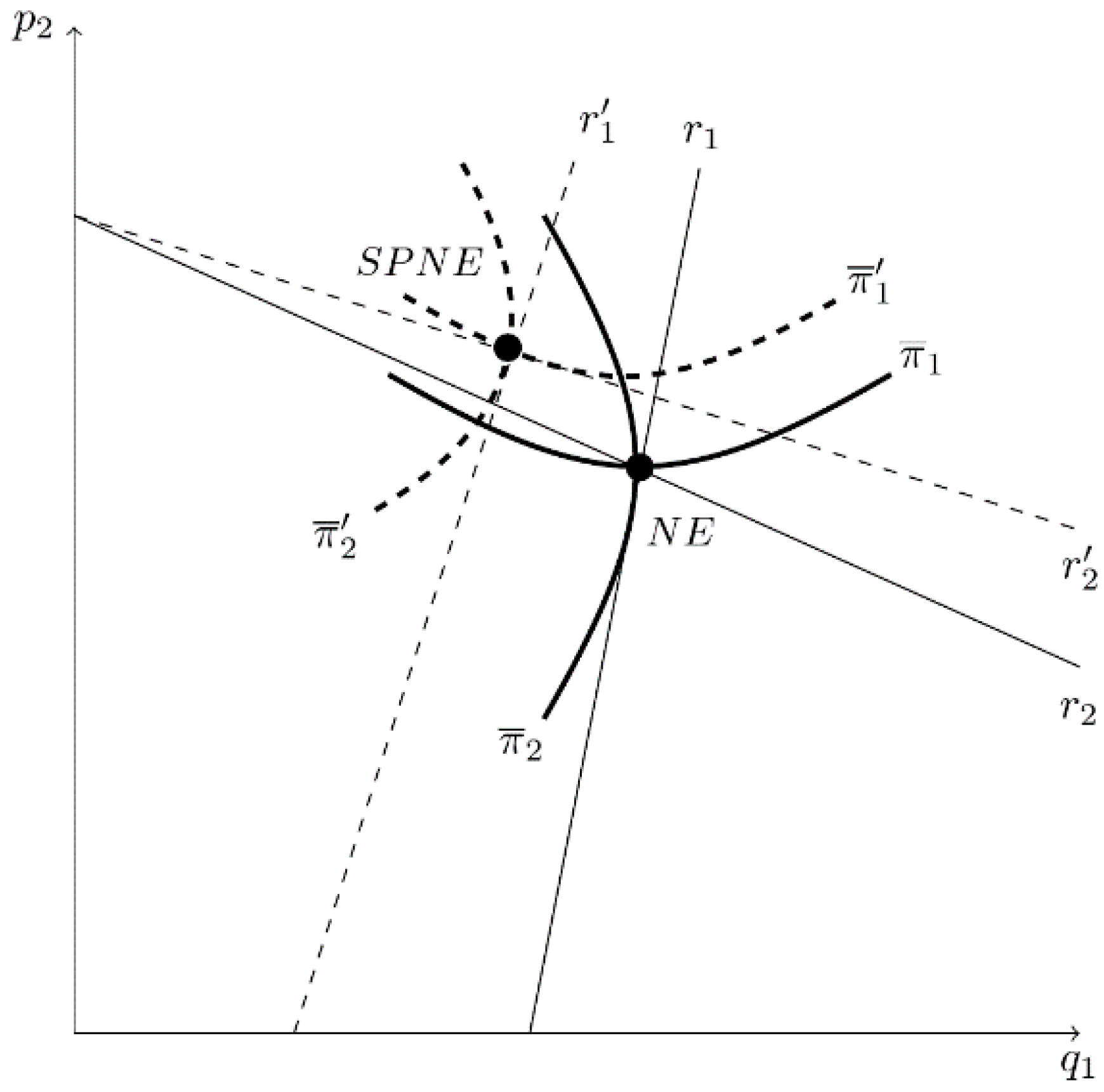
As in the previous models, backwards induction is used to obtain the SPNE. In stage II, the Nash equilibrium values are and . In stage I, firm i’s profit depends on first-stage choices, and , and the anticipated actions in the second period, such that . Figure 11 describes each firm’s best-reply curve and the simple Nash (Cournot–Bertrand) equilibrium, assuming no estimation bias (). Figure 11 also depicts firm 1’s iso-profit curve, which is convex to the -axis, and firm 2’s iso-profit curve, which is concave to the -axis. In this model, firm 1’s profit is greater for a higher iso-profit curve (i.e., the firm’s profit increases with ); firm 2’s profit is greater for an iso-profit curve that is further left (i.e., the firm’s profit increases as decreases).
Given that firms optimize over different choice variables, the effect of estimation bias on profit may differ by firm. Thus, we first consider the effect of bias for each individual firm before investigating the case where both owners have the option of hiring biased CEOs. Regarding the Cournot-type firm (firm 1):
Proposition 3.
Consider this two-stage game with Cournot–Bertrand competition in stage II and where only the Cournot-type firm has the option of hiring a biased CEO [, ] in stage I.
- A.
- If a change in has no direct effect on in the neighborhood of the simple Cournot–Bertrand outcome where , then firm 1 hires a CEO who overestimates the degree of product substitutability ().
- B.
- If a change in directly affects by shifting firm 2’s best-reply function, then the sign of CEO1’s estimation bias is indeterminate.
Proof.
Given that the underestimation of the degree of product substitutability induces CEO1 to increase output, in the neighborhood of the simple Cournot–Bertrand outcome where . As a result, and firm 1 hires a CEO who overestimates the degree of product substitutability ().
In this case, the sign of is indeterminant without knowing the sign and relative magnitude of the direct effect . □
When corresponds to output for firm 1 and price for firm 2, Equation (1) becomes the following for firm 1:
With profit maximization, ; therefore, the first set of terms on the right-hand side of the equality equals 0. Given that products are substitutes, . Because firm 2’s best-reply function has a negative slope in the Cournot–Bertrand model, .
- In the absence of a direct effect of on , the following is true:
- B.
- With a direct effect:
The intuition behind Part A of Proposition 3 is evident from Figure 11, where NE assumes no bias. If a marginal increase in , signifying an overestimation of product substitutability, causes to shift left and has no effect of , then firm 1’s profit rises as the equilibrium moves up to a point that is above the iso-profit curve 12. Thus, . Part B is relevant when the change also causes to shift. If the increase in causes to shift left (i.e., firm 2 behaves less aggressively by setting a lower price for a given level of ), then firm 1’s profit may increase, decrease, or remain the same depending on whether the new equilibrium is above, below, or on iso-profit curve . In this case, the sign of is indeterminate.
The following proposition considers the case where only the Bertrand-type firm (firm 2) can hire a biased CEO.
Proposition 4.
Consider this two-stage game with Cournot–Bertrand competition in stage II and where only the Bertrand-type firm has the option of hiring a biased CEO [] in stage I.
- A.
- If a change in has no direct effect on in the neighborhood of the simple Cournot–Bertrand outcome where , then firm 2 hires a CEO who overestimates the degree of product substitutability ().
- B.
- If a change in directly affects by shifting firm 1’s best-reply function, then the sign of CEO2’s estimation bias is indeterminate.
Proof.
Given that the underestimation of the degree of product substitutability causes CEO2 to increase the price, in the neighborhood of the simple Cournot–Bertrand outcome where . As a result, and firm 2 hires a CEO who overestimates the degree of product substitutability ().
In this case, the sign of is indeterminant without knowing the sign and magnitude of the direct effect . □
When corresponds to output for firm 1 and to price for firm 2, Equation (1) becomes the following for firm 2:
With profit maximization, and the first set of terms on the right-hand side of the equality equals 0. Given that products are substitutes, . Because firm 1’s best-reply function has a positive slope in the Cournot–Bertrand model, .
- In the absence of a direct effect of on , the following is true:
- B.
- With a direct effect:
Part A of Proposition 4 is evident from Figure 11 when NE assumes no bias. If a marginal increase in , signifying an overestimation of product substitutability, causes to shift left and has no effect on , then firm 2’s profit rises as the equilibrium moves down to a point that is left of the iso-profit curve 13. Thus, . Part B is relevant when the change also causes to shift. If the increase in causes to shift right (i.e., firm 1 behaves more aggressively by producing more output for a given ), then firm 2’s profit may increase, decrease, or remain the same depending on whether the new equilibrium is to the left of, to the right of, or on iso-profit curve . In this case, the sign of is indeterminate.
Finally, when the owners of both firms have the option of hiring a strategically biased CEOs in stage I, the resulting SPNE has the following characteristics.
Proposition 5.
Consider this two-stage game with Cournot–Bertrand competition in stage II and where both firms have the option of hiring a biased CEO in stage I.
- A.
- In the absence of direct effects in the neighborhood of the simple Cournot–Bertrand outcome where , both firms hire CEOs who overestimate the degree of product substitutability ().
- B.
- When direct effects are present, the sign of CEO estimation bias is indeterminate.
The proof of Part A follows from Propositions 3 and 414. It is difficult to verify Part B directly, but we use the linear model of Dixit [24] and Singh and Vives [25] to prove it indirectly.
In this specification, the firm demand equations depend on choice variables and are derived by solving Equations (2) and (3) for and . The true demand equations are:
The resulting profit equations are:
In the presence of bias, which occurs when CEOi believes that , CEOs expect the demand equations to be15:
The expected profit equations are:
We use backwards induction to obtain the SPNE. In stage II, CEOs simultaneously maximize expected profits with respect to their particular choice variable, for CEO1 and for CEO2.
Because the best-reply functions in stage II differ by firm, we examine them separately. Solving firm 1’s first-order condition for yields its best-reply function:
Figure 12 graphs this function when is on the horizontal axis and is on the vertical axis. In this model, has a positive slope. A decrease in (i.e., CEO1 underestimates product substitutability by a greater degree) causes to become steeper and its -intercept16 to shift right (e.g., shifting to in Figure 12). More importantly, unlike the linear specifications of the Cournot and Bertrand models, firm 1’s best reply depends on as well as . A decrease in causes firm 1’s best reply to become steeper and the -intercept to shift left, as is illustrated in Figure 13. That is, an underestimation of the degree of product substitutability by CEO2 causes firm 1 to behave less aggressively (i.e., firm 1 produces less output for a given ). We see that it is this influence of on firm 1’s best-reply function that drives the result in Part B of Proposition 5.
Firm 2’s best-reply function in the stage II problem derives from its first-order condition and is described below.
Figure 14 illustrates firm 2’s best reply. It has a negative slope, and a decrease in (i.e., the underestimation of strategic effects) causes to shift to . Firm 2’s best reply becomes flatter, while the -intercept remains constant at the simple monopoly price (). In the linear model, a change in has no effect on .
Solving the best-reply functions simultaneously for and yields Nash equilibrium values in stage II:
In stage I, owners simultaneously choose to maximize true profit, given anticipated CEO choices in stage II, and . Thus, owners anticipate profits to be:
In this game, there are two SPNE, identified as SPNE-A and SPNE-B17. Table 3 lists equilibrium values for SPNE-A and the simple Cournot–Bertrand outcome (NE). (The simple cartel and competitive outcomes are the same as in Table 1). Note that in this case, the parameter restrictions of the model [ and ] require that . This means that there can only be a mild degree of product differentiation (i.e., is sufficiently close to ). At SPNE-A, : it is optimal for owners to hire CEOs who underestimate the degree of product substitutability. In the limit, however, as : it pays the owner of the Bertrand-type firm to hire an unbiased CEO18. In addition, the presence of CEO bias reduces competition. For both firms, SPNE-A prices exceed NE prices but fall short of the cartel price.
Table 4 lists the optimal values for the equilibrium SPNE-B. (The simple cartel and competitive outcomes can be found in Table 1, and the simple Cournot–Bertrand outcome is the same as in Table 3). In this equilibrium, whether it pays an owner to hire a biased CEO depends on the degree of product differentiation and whether the firm competes in output or price. At this equilibrium:
- When , it is optimal for both owners to hire CEOs who underestimate the degree of product substitutability ().
- When , it is optimal for the owner of the Cournot-type firm to hire an unbiased CEO and the owner of the Bertrand-type firm to hire a CEO who underestimates product substitutability ().
- When (i.e., there is considerable product differentiation), it is optimal for the owner of firm 1 to hire a CEO who overestimates product substitutability and the owner of firm 2 to hire a CEO who underestimates product substitutability ().
- When , ; when , ; when , .
Unlike in the Cournot and the Bertrand models, it is impossible to know the direction of bias in SPNE-B without additional information. This is consistent with Part B of Proposition 5, because a change in causes the best-reply curves of both firms to shift. The fundamental prediction of the Cournot–Bertrand case is that an owner is likely to hire a CEO who overestimates strategic effects when the firm competes in output and there is a substantial degree of product differentiation.
Figure 15 provides an illustration when and . NE identifies the simple Cournot–Bertrand equilibrium in the absence of bias (). When owners have the option of hiring biased CEOs in stage I, each owner chooses to maximize profit given the best reply of its competitor. The SPNE is reached when this simultaneously holds for each owner and occurs where firm i’s iso-profit curve is tangent to firm j’s best-reply curve at SPNE. Identifying the SPNE relative to NE is difficult because shifts with changes in both and . That is, the increase in causes to become flatter and the -intercept to decrease. The decrease in causes to become steeper and the -intercept to decrease19. Thus, the resulting shift in is indeterminate. Figure 15 provides an example where overestimation of product substitutability by CEO1 and underestimation of product substitutability by CEO2 lead to a decrease in and an increase in . Thus, competition is diminished, and each firm earns greater profit20.
3. Summary of Results
This research demonstrates how the likelihood of CEO bias and the resulting welfare effect depend on market conditions. In the absence of strategic effects, as in perfect competition and monopoly, it is profit maximizing for owners to hire unbiased CEOs. In imperfectly competitive markets, however, the results depend on the mode of competition and on the effect of a CEO’s estimation bias on the behavior of its competitor.
Our duopoly model provides definitive results when the bias of one CEO does not affect the degree of bias of the other CEO, i.e., when the direct effect of bias on the competitor’s best-reply function is zero. These results are summarized in Table 5. With either Cournot or Bertrand competition in the product market, it is always in the interest of owners to hire CEOs who underestimate product substitutability. In a Cournot setting, this leads to greater production, which harms firms but increases welfare (consumer plus producer surplus). With Bertrand competition, this leads to higher prices and profits but lower welfare. Finally, in the asymmetric case of Cournot–Bertrand competition, it is optimal for owners to hire CEOs who overestimate product substitutability. In this setting, the Bertrand-type firm benefits but the effects of estimation bias on the Cournot-type firm’s profit and on welfare are indeterminate. As discussed in the previous section (Figure 3 and Figure 8), the motive for hiring a biased CEO is driven by the fact that firm i benefits from hiring a biased CEO because it profitably changes the behavior of firm j. In the Cournot model, it unambiguously lowers ; in the Bertrand model, it unambiguously raises .
When direct effects are present, however, the net benefit of hiring a biased CEO is inconclusive because it depends on the sign and magnitude of the direct effect, . Overall, the welfare effect of CEO bias is case-specific. The presence of CEO bias predicts a variety of possible outcomes, illustrating the difficulty of policy analysis in imperfectly competitive markets.
4. Conclusions
Previous studies by Blake et al. [8] and Rao and Simonov [9] find that firms appear to miscalculate the effectiveness of advertising. Rao and Simonov argue that this may be due to a principal–agent problem or the fact that management is unaware of the best methods for estimating the demand effect of advertising. We argue that there are conditions under which it is optimal for owners to hire CEOs who make biased estimates of demand conditions.
We develop a two-stage model where owners hire potentially biased CEOs in the first period and firms (CEOs) compete in output or price in the second period. In our application, CEO bias is associated with the estimation of the degree of substitutability between competing products. The model demonstrates that an owner’s decision to hire a biased CEO depends on the mode of competition and the strategic effect that one CEO’s bias has on its rival’s best-reply function (i.e., a direct effect).
In a non-strategic setting, the model predicts that it is optimal for owners to hire unbiased CEOs. In a strategic setting, clear results emerge when there are no direct effects. In this case, it is optimal for owners to hire CEOs who underestimate the degree of product substitutability when there is Cournot or Bertrand competition in the product market. With Cournot–Bertrand behavior, it is optimal for owners to hire CEOs who overestimate product substitutability. When there are direct effects, however, whether it is optimal to hire CEOs who are biased or unbiased depends on the direction and magnitude of these direct effects.
Our work contributes to the behavioral economics literature by providing the first model to explain why owners may prefer to hire CEOs who make systematic measurement errors. This result is consistent with Schelling’s [26] notion of the “rationality of irrationality”. That is, it may be perfectly rational (i.e., profit maximizing) for owners to hire irrational/biased CEOs. In addition, the model makes it clear that policy analysis is difficult given that the welfare effect of CEO bias depends on market conditions, particularly the mode of competition and the way in which CEO bias affects the best-reply functions of competitors.
In future research, the model could be extended in several ways. For example, owners might optimize over market share or reputation rather than profit21. In addition, firms frequently consider more than one choice variable. Following the approach used by Schroeder et al. [16] regarding overconfident CEOs, for example, the model could be extended to the case of two choice variables, such as output (or price) and advertising.
Author Contributions
Conceptualization, E.S., C.H.T. and V.J.T.; validation, E.S. and C.H.T.; formal analysis, V.J.T.; writing—original draft preparation, E.S., C.H.T. and V.J.T.; writing—review and editing, E.S., C.H.T. and V.J.T. All authors have read and agreed to the published version of the manuscript.
Funding
This research received no external funding.
Institutional Review Board Statement
Not applicable.
Informed Consent Statement
Not applicable.
Data Availability Statement
Not applicable.
Conflicts of Interest
The authors declare no conflict of interest.
| 1 | |
| 2 | |
| 3 | For a survey of the many theoretical applications and descriptions of other real-world examples of Cournot–Bertrand behavior, see Tremblay and Tremblay [20]. |
| 4 | Consistent with the overconfidence literature, we investigate the cases of perfect competition, monopoly, and duopoly. In an imperfectly competitive setting, the main implications of the model would be unaffected by considering n instead of 2 firms, because the resulting changes in best-reply functions due to estimation bias remain the same. Thus, to simplify the analysis, we focus on duopoly. |
| 5 | As discussed in Amir and Grilo [21] and Tremblay and Tremblay [20], this means that firm demand has a negative slope, demand cannot be too convex, a firm’s own strategic variable has a greater effect (in absolute value) on its demand than its competitor’s strategic variable. With Cournot competition, where both firms compete in output, the choice variables are strategic substitutes (i.e., best-reply or reaction functions have a negative slope). With Bertrand competition, where both firms compete in price, the choice variables are strategic complements (i.e., best-reply functions have a positive slope). With Cournot–Bertrand competition, where one firm competes in output and the other firm competes in price, the choice variables are strategic complements for the Cournot-type firm and are strategic substitutes for the Bertrand-type firm. The best-reply function has a positive slope for the Cournot-type firm and a negative slope for the Bertrand-type firm, as discussed in Tremblay and Tremblay [20,22]. For simplicity, our specific examples assume that firms have symmetric inverse demand and cost functions. |
| 6 | One possible mechanism is contagion where bias breeds bias, such that . |
| 7 | The reverse is true when CEOi overestimates product substitutability (i.e., . In this case, the CEO believes that firm j is a tougher or closer competitor than is actually true. This induces the CEO to decrease output/price from the simple Nash equilibrium outcome, assuming no direct effect. |
| 8 | We solve for in order to make it easier to understand the graph of each firm’s best-reply function, with (or ) on the vertical axis and (or ) on the horizontal axis. |
| 9 | In the limiting case where CEO1 believes that products 1 and 2 are unrelated: , firm 1’s best-reply curve is vertical, and the firm 1 produces the simple monopoly level of output . |
| 10 | The simple cartel outcome assumes symmetry (i.e., ). In the simple competitive outcome, price equals marginal cost which is zero in the case. All “simple” (competitive, Cournot, and cartel) outcomes assume no CEO bias. |
| 11 | This also benefits firm 2. |
| 12 | This benefits firm 2 as well, as the new equilibrium is left of iso-profit curve . |
| 13 | This harms firm 1, however, as the new equilibrium is below iso-profit curve . |
| 14 | Figure 11 makes it clear that in the absence of direct effects, overestimation by both CEOs causes and to shift left, causing SPNE to be to the left of NE. This unambiguously increases firm 2’s profit but may increase or decrease firm 1’s profit depending on whether the SPNE is above or below iso-profit curve . |
| 15 | Unlike in the linear examples of the Cournot and Bertrand models that have direct effects, firm 1’s expected demand depends on both and , which causes a direct effect in the Cournot–Bertrand model. |
| 16 | The -intercept is . |
| 17 | In this model, firm 1 earns greater profit in equilibrium A, and firm 2 earns greater profit in equilibrium B. If firms were to cooperate, joint profits are greater in case A. Of course, if firms were to cooperate, they would most prefer the cartel outcome. |
| 18 | As previous studies have found, the Cournot-type firm earns greater profit than the Bertrand-type firm, assuming that the Cournot-type firm does not face substantially higher costs. In addition, the presence of CEO bias reduces competition. |
| 19 | The decrease in causes to become flatter and the -intercept is unchanged. |
| 20 | This is evident by the fact that firm 1 is able to move to a higher iso-profit curve (from to ) and firm 2 is able to move to an iso-profit curve that is further to the left (from to ). |
| 21 | We wish to thank an anonymous referee for suggesting this alternative specification. |
References
- Ellison, G. Bounded Rationality in Industrial Organization. Econom. Soc. Monogr. Natl. Bur. Econ. Res. 2006, 42, 142. [Google Scholar]
- Armstrong, M.; Huck, S. Behavioral Economics as Applied to Firms: A Primer. Compet. Policy Int. 2010, 6, 3–45. [Google Scholar] [CrossRef]
- Spiegler, R. Bounded Rationality and Industrial Organization; Oxford University Press: Oxford, UK, 2011. [Google Scholar]
- Grubb, M. Overconfident Consumers in the Marketplace. J. Econ. Perspect. 2015, 29, 9–36. [Google Scholar] [CrossRef] [Green Version]
- Dhami, S. The Foundations of Behavioral Economic Analysis; Oxford University Press: Oxford, UK, 2016. [Google Scholar]
- Tremblay, V.J.; Schroeder, E.; Tremblay, C.H. (Eds.) Handbook of Behavioral Industrial Organization; Edward Elgar: Cheltenham, UK, 2018. [Google Scholar]
- Dixon, H. Almost-Maximization as a Behavioral Theory of the Firm: Static, Dynamic and Evolutionary Perspectives. Rev. Ind. Organ. 2020, 56, 237–258. [Google Scholar] [CrossRef] [Green Version]
- Blake, T.; Nasko, C.; Tadelis, S. Consumer Heterogeneity and Paid Search Effectiveness: A Large Scale Field Experiment. Econometrica 2015, 83, 155–174. [Google Scholar] [CrossRef]
- Rao, J.M.; Simonov, A. Firms’ Reactions to Public Information on Business Practices: The Case of Search Advertising. Quant. Mark. Econ. 2019, 17, 105–134. [Google Scholar] [CrossRef]
- Malmendier, U.; Tate, G. Behavioral CEOs: The Role of Managerial Overconfidence. J. Econ. Perspect. 2015, 29, 37–60. [Google Scholar] [CrossRef] [Green Version]
- Goel, A.M.; Thakor, A.V. Overconfidence, CEO Selection, and Corporate Governance. J. Financ. 2008, 63, 2737–2784. [Google Scholar] [CrossRef]
- Englmaier, F. Managerial Optimism and Investment Choice. Manag. Decis. Econ. 2010, 31, 303–310. [Google Scholar] [CrossRef] [Green Version]
- Englmaier, F. Commitment in R&D Tournaments via Strategic Delegation to Overoptimistic Managers. Manag. Decis. Econ. 2011, 32, 63–69. [Google Scholar]
- Campbell, T.C.; Gallmeyer, M.; Johnson, S.A.; Rutherford, J.; Brooke, W.S. CEO Optimism and Forced Turnover. J. Financ. Econ. 2011, 101, 695–712. [Google Scholar] [CrossRef]
- Englmaier, F.; Reisinger, M. Biased Managers as Strategic Commitment. Manag. Decis. Econ. 2014, 35, 350–356. [Google Scholar] [CrossRef]
- Schroeder, E.; Tremblay, C.H.; Tremblay, V.J. Confidence Bias and Advertising in Imperfectly Competitive Markets. Manag. Decis. Econ. 2021, 42, 885–897. [Google Scholar] [CrossRef]
- Schroeder, E.; Tremblay, C.H.; Tremblay, V.J. CEO Confidence and Mode of Competition; Working Paper; Department of Economics, Oregon State University: Corvallis, OR, USA, 2021. [Google Scholar]
- Schroeder, E.; Tremblay, C.H.; Tremblay, V.J. CEO Confidence and Strategic Choice: A General Framework. J. Appl. Econ. 2022; in press. [Google Scholar]
- Bylka, S.; Komar, J. Cournot-Bertrand Mixed Oligopolies. In Warsaw Fall Seminars in Mathematical Economics, 1975; Los, M.W., Los, J., Wieczorek, A., Eds.; Springer: New York, NY, USA, 1976; pp. 22–33. [Google Scholar]
- Tremblay, C.H.; Tremblay, V.J. Oligopoly Games and the Cournot-Bertrand Model: A Survey. J. Econ. Surv. 2019, 33, 1555–1577. [Google Scholar] [CrossRef]
- Amir, R.; Grilo, I. Stackelberg versus Cournot Equilibrium. Games Econ. Behav. 1999, 26, 1–21. [Google Scholar] [CrossRef]
- Tremblay, V.J.; Tremblay, C.H. New Perspectives on Industrial Organization: With Contributions from Behavioral Economics and Game Theory; Springer: New York, NY, USA, 2012. [Google Scholar]
- D’Aspremont, C.; Gérard-Varet, L.A. Stackelberg-Solvable Games and Pre-Play Communication. J. Econ. Theory 1980, 23, 201–217. [Google Scholar] [CrossRef]
- Dixit, A. A Model of Duopoly Suggesting a Theory of Entry. Bell J. Econ. 1979, 10, 20–32. [Google Scholar] [CrossRef]
- Singh, N.; Vives, X. Price and Quantity Competition in a Differentiated Duopoly. Rand J. Econ. 1984, 15, 546–554. [Google Scholar] [CrossRef]
- Schelling, T.C. The Strategy of Conflict; Oxford University Press: New York, NY, USA, 1960. [Google Scholar]
Figure 1.
Firm 1’s Best-Reply Curve (r1) in the Cournot Model when CEO1 Underestimates Product Substitutability.
Figure 1.
Firm 1’s Best-Reply Curve (r1) in the Cournot Model when CEO1 Underestimates Product Substitutability.

Figure 2.
Best-Reply Curves, Iso-Profit Curves, and the Nash Equilibrium (NE) in the Simple Cournot Model.
Figure 2.
Best-Reply Curves, Iso-Profit Curves, and the Nash Equilibrium (NE) in the Simple Cournot Model.

Figure 3.
Owner 1’s Incentive to Hire a CEO Who Underestimates Product Substitutability in the Cournot Model.
Figure 3.
Owner 1’s Incentive to Hire a CEO Who Underestimates Product Substitutability in the Cournot Model.

Figure 4.
The Subgame-Perfect Nash Equilibrium (SPNE) When Owners Hire CEOs Who Underestimate Product Substitutability.
Figure 4.
The Subgame-Perfect Nash Equilibrium (SPNE) When Owners Hire CEOs Who Underestimate Product Substitutability.

Figure 5.
Owner 1’s Incentive to Hire a CEO Who Overestimates Product Substitutability in the Cournot Model When Overestimation Affects the Best-Reply Curves of Both Firms.
Figure 5.
Owner 1’s Incentive to Hire a CEO Who Overestimates Product Substitutability in the Cournot Model When Overestimation Affects the Best-Reply Curves of Both Firms.

Figure 6.
Firm 1’s Best-Reply Curve in the Bertrand Model When CEO1 Underestimates Product Substitutability.
Figure 6.
Firm 1’s Best-Reply Curve in the Bertrand Model When CEO1 Underestimates Product Substitutability.

Figure 7.
Best Reply Curves, Iso-Profit Curves, and the NE in the Simple Bertrand Model.

Figure 8.
Owner 1’s Incentive to Hire a CEO Who Underestimates Product Substitutability in the Bertrand Model.
Figure 8.
Owner 1’s Incentive to Hire a CEO Who Underestimates Product Substitutability in the Bertrand Model.

Figure 9.
The SPNE When Owners Hire CEOs Who Underestimate Product Substitutability in the Bertand Model.
Figure 9.
The SPNE When Owners Hire CEOs Who Underestimate Product Substitutability in the Bertand Model.

Figure 10.
Owner 1’s Incentive to Hire a CEO Who Overestimates Product Substitutability in the Bertrand Model When Overestimation Affects the Best-Reply Curves of Both Firms.
Figure 10.
Owner 1’s Incentive to Hire a CEO Who Overestimates Product Substitutability in the Bertrand Model When Overestimation Affects the Best-Reply Curves of Both Firms.

Figure 11.
Best-Reply Curves, Iso-Profit Curves, and the NE in the Simple Cournot-Bertrand Model.

Figure 12.
Firm 1’s Best-Reply Curve in the Cournot-Bertrand Model When CEO1 Underestimates Product Substitutability.
Figure 12.
Firm 1’s Best-Reply Curve in the Cournot-Bertrand Model When CEO1 Underestimates Product Substitutability.

Figure 13.
Firm 1’s Best-Reply Curve in the Cournot-Bertrand Model When CEO2 Underestimates Product Substitutability.
Figure 13.
Firm 1’s Best-Reply Curve in the Cournot-Bertrand Model When CEO2 Underestimates Product Substitutability.

Figure 14.
Firm 2’s Best-Reply Curve in the Cournot-Bertrand Model When CEO2 Underestimates Product Substitutability.
Figure 14.
Firm 2’s Best-Reply Curve in the Cournot-Bertrand Model When CEO2 Underestimates Product Substitutability.

Figure 15.
The SPNE When CEO1 Overestimates and CEO2 Underestimates Product Substitutability in the Cournot-Bertrand Model.
Figure 15.
The SPNE When CEO1 Overestimates and CEO2 Underestimates Product Substitutability in the Cournot-Bertrand Model.


Table 1.
Equilibrium values when firms compete in output.
| SPNE | Competition | Simple Cournot (NE) | Simple Cartel | |
|---|---|---|---|---|
| 1 | 1 | 1 | ||
| 0 | ||||
| 0 |
Table 2.
Equilibrium values when firms compete in price.
| SPNE | Simple Bertrand (NE) | |
|---|---|---|
| 1 | ||
Note: . The competitive and simple cartel solutions are the same as in Table 1.
Table 3.
Equilibrium values in the Cournot–Bertrand (C–B) model: SPNE-A.
| SPNE | Simple C–B (NE) | |
|---|---|---|
| 1 | ||
| 1 | ||
Note: Firm 1 competes in output and firm 2 competes in price. This SPNE requires that that . The competitive and simple cartel solutions are the same as in Table 1.
Table 4.
Equilibrium values in the Cournot–Bertrand (C–B) model: SPNE-B.
| SPNE | |
|---|---|
Note: Firm 1 competes in output and firm 2 competes in price. . . . .
Table 5.
The mode of competition, CEO estimation bias (ϕ), profit (π), and welfare (producer plus consumer surplus).
Table 5.
The mode of competition, CEO estimation bias (ϕ), profit (π), and welfare (producer plus consumer surplus).
| Mode of Competition | Estimation Bias of Product Substitutability | Change in | ||
|---|---|---|---|---|
| π1 | π2 | Welfare | ||
| Non-Strategic Settings: | ||||
| Monopoly | Unbiased (ϕi = 1) | (0) | (0) | (0) |
| Perfect Competition | Unbiased (ϕi = 1) | (0) | (0) | (0) |
| Strategic Settings: | ||||
| Cournot | Underestimate (ϕi < 1) | (−) | (−) | (+) |
| Bertrand | Underestimate (ϕi < 1) | (+) | (+) | (−) |
| Cournot-Bertrand | Overestimate (ϕi > 1) | Indeterminate | (+) | Indeterminate |
Publisher’s Note: MDPI stays neutral with regard to jurisdictional claims in published maps and institutional affiliations. |
© 2022 by the authors. Licensee MDPI, Basel, Switzerland. This article is an open access article distributed under the terms and conditions of the Creative Commons Attribution (CC BY) license (https://creativecommons.org/licenses/by/4.0/).
Share and Cite
MDPI and ACS Style
Schroeder, E.; Tremblay, C.H.; Tremblay, V.J. CEO Bias and Product Substitutability in Oligopoly Games. Games 2022, 13, 28. https://0-doi-org.brum.beds.ac.uk/10.3390/g13020028
AMA Style
Schroeder E, Tremblay CH, Tremblay VJ. CEO Bias and Product Substitutability in Oligopoly Games. Games. 2022; 13(2):28. https://0-doi-org.brum.beds.ac.uk/10.3390/g13020028
Chicago/Turabian StyleSchroeder, Elizabeth, Carol Horton Tremblay, and Victor J. Tremblay. 2022. "CEO Bias and Product Substitutability in Oligopoly Games" Games 13, no. 2: 28. https://0-doi-org.brum.beds.ac.uk/10.3390/g13020028
Note that from the first issue of 2016, this journal uses article numbers instead of page numbers. See further details here.