Inequalities between Others Do Matter: Evidence from Multiplayer Dictator Games

Abstract

Social motives are frequently used to explain deviations from selfishness in non-strategic settings such as the Dictator Game. Previous research has mainly focused on two-player games; the workings of social motives in multiplayer Dictator Games are less well understood. A core feature of multiplayer games is that players can consider inequalities between others, in addition to outcomes that have two-player analogues, such as social efficiency and the inequality between self and others. We expect that existing models of social motives can be improved if players are allowed to consider the inequality between others. Results from two laboratory experiments confirm this: motives for the inequality between others were found, and these motives could not be reduced to motives with dyadic analogues. Explorative analyses show that our findings are robust to a number of potential misspecifications: motives for the inequality between others were also found when utility included non-linear evaluations of inequality, and when alternative types of self-other comparison mechanisms were modeled. Thus, to adequately capture social motives in multiplayer games, models should account for the complexities of the multiplayer setting. We speculate that our findings also hold for strategic games; but further research is needed to elucidate this.

1. Introduction

In the summer of 2015, when the full scale of Europe’s refugee crisis became apparent to many, Hungarian prime minister Viktor Orbán proposed to give Syria’s neighboring countries three billion euros in financial aid. Hungary’s recent political course is often characterized as “anything but left”—see for example Szikra’s review [1]—therefore, this apparent altruistic gesture was surprising. But Orbán’s proposal did not reveal pure altruism; it signaled clear Hungarian self-interest: an increased welfare could help Syria’s neighbors absorb more refugees; less inequality between Europe and the Middle East could make Europe a comparatively less attractive destination; and less inequality within and between Middle Eastern societies could even mitigate existing conflicts. Orbán’s proposals alone will, arguably, not solve the refugee crisis; but his statements do exemplify that overt distributional considerations can serve one’s ultimate self-interest.

Deviations from pure material self-interest have received much scholarly attention. The Dictator Game (DG) has become the prototypical tool to study the motives behind such non-selfish behavior. In the DG a decision-maker—the Dictator—is asked to choose between options that differ in the amount of monetary payoffs allocated to self and one or more other players. The game is one-shot, choices are made anonymously, and the other players must accept the Dictator’s decision [2]. This eliminates the need for strategic considerations [3]: Dictators can maximize selfish outcomes without having to fear future retaliation. Nevertheless, countless experiments have shown that non-selfish DG-choices are frequent [4,5]. Many individuals thus appear to have a baseline-level of social motives [3,6,7,8].

Much research has focused on social motives in two-player DGs. To explain the frequent deviations from selfishness, non-selfish utility functions have been introduced to capture how the other player’s material payoffs enter the utility of ego [8,9,10]. A summary of Schulz and May [11] showed that two-player models typically contain combinations of motives regarding own material payoffs (selfishness), joint payoffs for self and other (efficiency), payoffs received by the other player (social efficiency), and the inequality between payoffs for self and payoffs for the other (self-centered inequality). Multiplayer DGs have been studied increasingly in the last decades, and attempts have been made to generalize dyadic motives to the multiplayer setting [12,13,14]. But such generalizations are not straightforward. First, an extensive comparison [5] showed that Dictators shared significantly more in games with multiple recipients. Group size may thus influence the strength of social motives1. Secondly, recent four-player experiments showed that the amount of sharing varied according to the decision-maker’s (earned) economic status [13,15]. The mechanisms that drive non-selfish choices may thus be considerably more complex in multiplayer games.

A distinctive feature of the multiplayer setting is that decision-makers can face dilemmas regarding the distribution of payoffs between others, irrespective of (social) efficiency and self-centered inequality. Multiplayer DGs can be used to assess the comparative importance of such a non-self-centered inequality motive, but studies on this matter have been scarce. Some prominent models have simply assumed that the non-self-centered inequality motive is negligible, or reduces to more basic types of motives2. For example, decision-makers in the ERC model of Bolton and Ockenfels [19] can consider their own payoffs and their relative position with respect to the group average (i.e., the social reference point), but not the inequality that may exist within the group. Similarly, the inequality-aversion model of Fehr and Schmidt [20] distinguishes different types of self-centered inequality motives (envy and guilt), but the model also assumes that individuals ignore the inequality between other players.

The social welfare model of Charness and Rabin [14] and the efficiency-maximin model of Engelmann and Strobel [21] do allow considerations for the distribution of goods between others. However, empirical tests have been limited to three-player games, which have inherent confounds. According to the social welfare model, individuals are motivated to increase the total amount of payoffs for all others, and favor distributions that progressively improve the conditions of the worst-off. Charness and Rabin [14] tested the model in three-player DGs in which decision-makers could choose between an egalitarian option where self and two others received 575 points each, and an unequal option, where self received 900 points, and the two other players received 300 and 600 points respectively. Self-interested decision-makers would choose the second option, yet results showed that the majority (54%) chose the first option. But as the authors noted themselves: these results do not prove the existence of social welfare motives: considerations for social efficiency, self-centered inequality, or non-self-centered inequality could explain these choices as well. The model of Engelmann and Strobel [21] assumes that decision-makers want to increase social efficiency and minimize the largest payoff-inequality between self and others (i.e., a maximin motive). The model was tested on a number of three-player taxation DGs. In these games, decision-makers had middle-class positions, and were asked to choose between options with different allocations of payoffs between the other players. Results showed that many effectively transferred payoffs from rich to poor, which suggests a maximin motive; but these results are again troubled by confounds.

This research aims to study social motives in the multiplayer DG, and in particular to assess whether choices can be explained better with models that take non-self-centered inequality motives into account. Our review of previous studies showed that three-player DGs have inherit confounds, therefore we focus on the four-player DG—the added recipient allows us to better disentangle multiple types of motives. Confounds can be eliminated by holding certain (irrelevant) selfish or social consequences constant, but this should be done with care. Engelmann and Strobel [21] for example eliminated selfish motives by fixing the material payoffs allocated to the decision-maker across the DG’s options. This allowed them to show the existence of the inequality-aversion motive in isolation, but their games lost their resemblance to real-world taxation problems (which generally involve at least some immediate efficiency-loss in the form of administrative costs). Moreover, if games allow decision-makers to influence social outcomes “for free”, it becomes impossible to quantify a motive’s strength. We strive to compare the relative importance of different types of selfish and social motives; this requires DGs with trade-offs between selfish and social outcomes.

Our study is structured as follows. First, we theorize why it is relevant to model non-self-centered inequality motives. Secondly, we present a utility function that incorporates this motive in addition to motives regarding social efficiency and self-centered inequality. This model can be applied to two-player and multiplayer games, and contains a number of the aforementioned models as special cases. Thirdly, we estimate the model on data from two controlled experiments. We assess its comparative performance and interpret its parameters. Fourthly, we conduct exploratory analyses to assess whether our findings are robust to violations of our modeling assumptions; specifically, we consider non-linearities and alternative comparison mechanisms in the evaluation of inequalities. Finally, we discuss the implications of our findings, and suggest directions for further research.

2. Theory

That the multiplayer DG makes it possible to reveal the non-self-centered inequality motive is not a sufficient reason to assume that the motive exists, nor that the motive matters to such a degree that models should incorporate it. Why should we consider non-self-centered inequality motives, and make models that are currently elegant and parsimonious, more complex and less elegant? To answer this question we first review a number of theoretical foundations for dyadic motives. Many types of dyadic motives follow from the assumption that at least some individuals have a distaste for unfavorable comparisons to others (i.e., envy), and the assumption that there are widely shared beliefs that inequalities cause conflict between the individuals with unequal resources. We then argue that the non-self-centered inequality motive follows from a trivial additional assumption, namely that conflicts can have consequences to third parties. Finally we argue that the aforementioned strategic mechanisms apply even for non-strategic games such as the DG.

2.1. Envy

Envy is ubiquitous, both in real life and in the laboratory. Dictators frequently choose to improve a relative disadvantage, even at the expense of their absolute payoffs [20]; and recipients in the Ultimatum Game frequently reject unfair offers, even if the consequence is that nobody receives anything [22]. Smith and Kim [23] provide an extensive evolutionary explanation for envy, and recent neuro-imaging studies have showed that the human brain is indeed “hard-wired” to detect, dislike, and diminish unfavorable social comparisons: in healthy subjects, brain regions associated with pain activate under conditions of disadvantageous inequality [24], whereas brain regions associated with pleasure activate under conditions of equality [25]. Envious choices reveal that the expected utility gains of a (subjective) increase in relative position outweigh the importance of expected material losses; such choices are not irrational, as long as one includes envious considerations in the utility function. Many models of social motives have acknowledged this, and take some form of envy into account [19,20].

2.2. Inequality and Conflict

Individuals in an advantageous position can be the object of envious acts of disadvantaged others. A rich person may therefore decide to donate a small amount of personal wealth to charity out of fear that the disadvantaged might otherwise take all the wealth illegitimately. History contains numerous examples to show that people will ultimately resort to (violent) conflicts to secure a more equal outcome [26,27]. The belief that inequality causes conflict is widespread: a large survey of US citizens [28], for example, showed that a majority of respondents (55%) agreed with the statement that “More equality of incomes would avoid conflicts between people at different levels.” A conflict-averse decision-maker thus has a strategic incentive to increase social efficiency and decrease advantageous inequality to the point that conflict is averted3. But conflicts do not affect only those that directly take part in them; the consequences of conflict often spill-over to third parties. Wars can burden countries unrelated to the conflict with refugees [29] and destabilize global financial markets [30,31]. Similarly, conflicts within organizations—for example, over inequalities in compensation—can severely impact organizational outcomes [32]. And even the expectation of conflict can drive insurance costs upwards. For a conflict-averse decision-maker it is therefore not only rational to improve the conditions of disadvantaged others (i.e., to maximize social efficiency or to minimize self-centered inequality), but also to minimize the inequality between them.

If all decision-makers were conflict-averse, there would probably be less inequality. But some would argue that such a society would also be less productive. It is apparent that neither inequalities nor conflict are universally disliked. First, there is the occasional anti-social “psychopath” that derives positive utility from inequalities and conflicts per se. But besides such deviant individuals, societies have entrepreneurs for whom a modest degree of inequality is instrumental in motivating their workforce. Kluegel and Smith [28] found that 72% of the respondents in their survey supported the statement that “Incomes should not be made more equal, since that would keep people from dreaming of someday becoming a real success”; and 63% supported the statement that “If incomes were more equal, nothing would motivate people to work hard.” Secondly, there are people that directly benefit from the conflicts that inequality can generate: wars benefit arms dealers just as crime legitimizes law-enforcement spending. Workplace conflicts provide work for legal professionals, just as family conflicts do for therapists, counselors, and social workers. For those who profit from conflict, it is rational to maintain inequalities; and for some tertius gaudentes [33], it can even be tempting to increase them.

2.3. Strategic Considerations in a Non-Strategic Setting: A Theoretical Paradox

Envy and conflict orientation may explain overt social motives in strategic settings with repeated interactions such as the political arena, the organization, and the family. But why should these factors matter to a non-strategic setting such as the DG? Players can arguably understand that the game is non-strategic: the DG is simple in itself, and the instructions make it obvious that strategic reasoning is unnecessary; and we can likewise assume that DG-players know that the game provides no opportunities for conflict. We resolve the theoretical paradox by making the additional assumptions (1) that players bring their individual characteristics (i.e., personality, dispositions, internalized norms) to the game [34]; (2) that these characteristics are at least partly associated with the players’ orientation towards conflict; and (3) that these characteristics influence the players’ behavior, even in games that lack the need for strategic considerations.

These assumptions are inconvenient for the model builder, but they do reflect a more realistic view on the nature of human behavior than the view that decision-makers are tabulae rasae: behavior is a function of both personal and situational factors [35,36]. An innovative study by Voors et al. [37] showed that individuals indeed bring their dispositions to the laboratory experiment. The study involved a field experiment on 300 Burundi households from 35 communities that had endured violent tribal clan conflicts for years. Results showed that even after accounting for factors that may have selected subjects into conflict, exposure to the conflict predicted pro-social choices in subsequent non-strategic experimental games. This study confirms that individual dispositions can spill-over into subsequent non-strategic experiments, and that such dispositions can be contingent on prior conflict experience.

3. Model

In multiplayer DGs, Dictators choose between options that vary in the amount of virtual tokens (x) assigned to self (i) and other players (j, k, etc.). A rational Dictator evaluates the options according to a personal function that converts material payoffs to effective utilities, and then chooses the option that maximizes utility [7]. We define utility as a linear combination of the option’s selfish and social consequences (X), weighed by the decision-maker’s motives (${\beta }_{\mathrm{i}}$):

$$\mathrm{U}\left(X|{\beta }_{\mathrm{i}}\right)\equiv X{\beta }_{\mathrm{i}}.$$

What selfish and social consequences should be included in our model? Previous research has shown that decision-makers in small-scale DGs consider social efficiency [21,38], as well as advantageous and disadvantageous inequality [20,22]. Our theory suggests that for the multiplayer setting, inequalities between others matter as well. It seems straightforward to construe a four-parameter model with corresponding terms for all aforementioned motives, but such ad-hoc combinations can create identification problems. Engelmann [39] showed that this already happens if one were to combine social efficiency motives and the two inequality aversion motives from the Fehr and Schmidt-model (i.e., even without introducing a term for non-self-centered inequality). The resulting three-parameter model is not identified, and reduces to a two-parameter model without the efficiency motive, or an equivalent two-parameter model with an efficiency-motive and a term that combines advantageous and disadvantageous inequality motives into one term.

We used the latter type as our reference model to expand with a term for non-self-centered inequality, but we acknowledge that this was an entirely arbitrary choice between two equivalent models.

Table 1. Linear Terms for Selfish and Social Consequences in Multiplayer Dictator Games (DGs).

	Abbreviation	Term	Weights
Selfish outcomes	${\mathrm{X}}^{\mathrm{S}}$	${\mathrm{x}}_{\mathrm{i}}^{}$	${\beta }_i^{\mathrm{s}}=1$
Social efficiency	${\mathrm{X}}^{\mathrm{Se}}$	${\overline{\mathrm{x}}}_{-\mathrm{i}}^{}$	${\beta }_i^{\mathrm{Se}}$
Self-centered inequality	${\mathrm{X}}^{\mathrm{Is}}$	$\frac{1}{\left(n-1\right)}{\displaystyle \sum }_{\mathrm{i}\ne \mathrm{j}}\left|{\mathrm{x}}_{\mathrm{i}}-{\mathrm{x}}_{\mathrm{j}}\right|$	${\beta }_i^{\mathrm{Is}}$
Non-self-centered inequality	${\mathrm{X}}^{\mathrm{Ins}}$	$\frac{2}{\left(n-1\right)\left(\mathrm{n}-2\right)}{\displaystyle \sum }_{\mathrm{i}\ne \mathrm{j},\mathrm{i}\ne \mathrm{k},\mathrm{j}\ne \mathrm{k}}\left|{\mathrm{x}}_{\mathrm{j}}-{\mathrm{x}}_{\mathrm{k}}\right|$	${\beta }_i^{\mathrm{Ins}}$

Note: The subscript i refers to the DG’s decision-maker; the subscripts j and k refer to other players; the total number of players is denoted by n.

summarizes how we conceptualized4 selfish and social consequences. Selfish outcomes reflect the tokens allocated to self; social efficiency refers to the average amount received by the other players; self-centered inequality refers to the average pairwise distance between self and others; non-self-centered inequality refers to the average distance between all pairs of others.

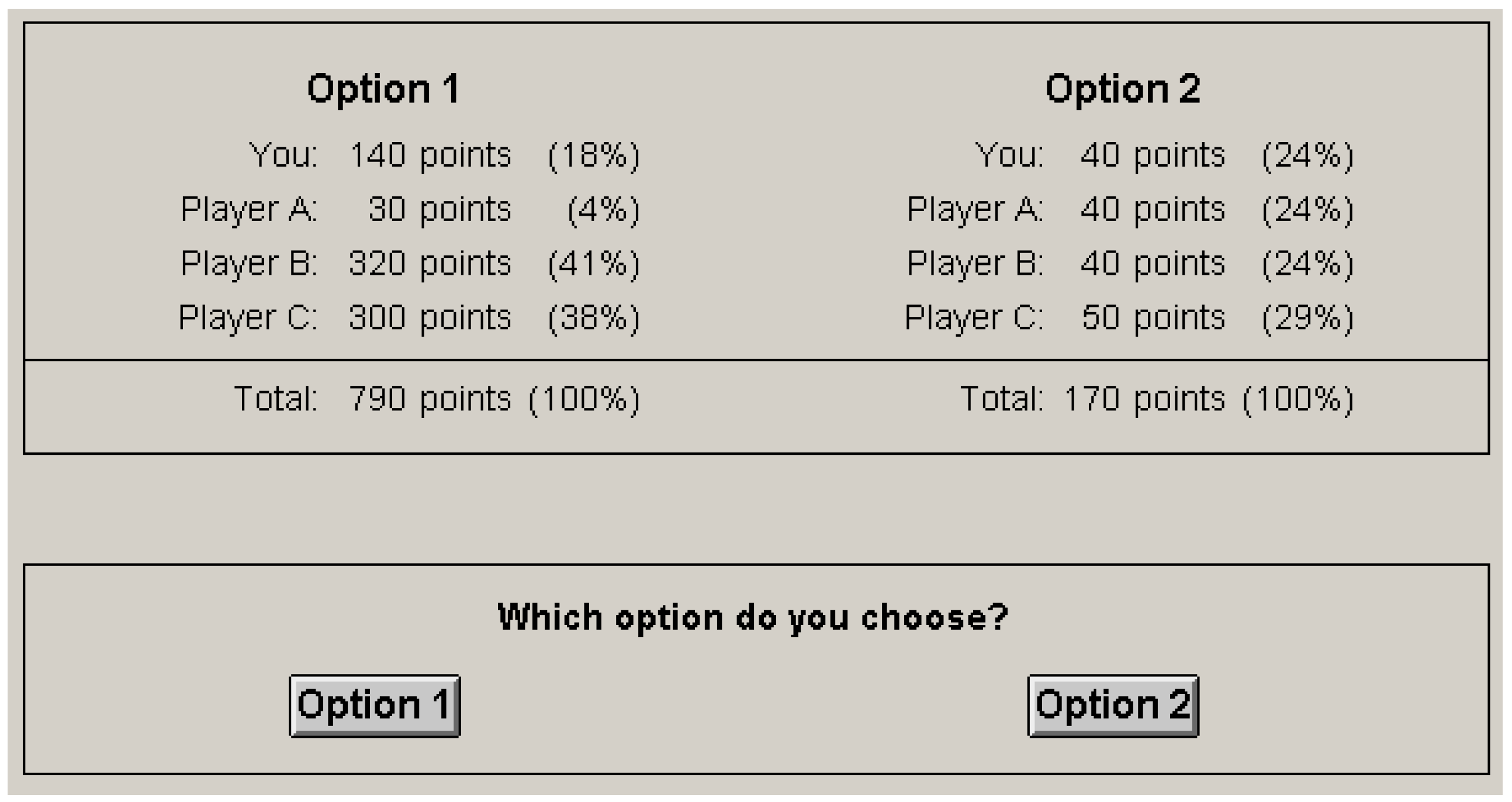
Qualitatively, the parameters in our model can be interpreted as follows: if a subject has ${\beta }_i^{\mathrm{Se}}=0$, she is indifferent to social efficiency; if she has ${\beta }_i^{\mathrm{Se}}<0$, she dislikes it; and if she has ${\beta }_i^{\mathrm{Se}}>0$, she prefers it. The parameters ${\beta }_i^{\mathrm{Is}}$ and ${\beta }_i^{\mathrm{Ins}}$ are interpretable in a similar manner: ${\beta }_i^{\mathrm{Is}}<0$ implies aversion to self-centered inequality, etc. Quantitatively, the parameters are interpretable as follows. First, we note that in our models, the weight of selfish outcomes is always fixed to 1. This causes social outcomes to be scaled relative to selfish outcomes. Suppose that a rational decision-maker is averse to non-self-centered inequality and has ${\beta }_i^{\mathrm{Ins}}$ = −0.2. Suppose now that she is asked to play a DG that contains a dilemma between selfishness and social outcomes. The two DG-options yield positive payoffs for all players, and are construed such that they differ only in the amount of selfish payoffs $\left({\mathrm{X}}^{\mathrm{S}}\right)$ and the amount of non-self-centered inequality $\left({\mathrm{X}}^{\mathrm{Ins}}\right)$. Option 1 has high selfish payoffs, but also a high degree of inequality between receivers; Option 2 has low selfish payoffs, but also a low degree of inequality between receivers. According to the DG’s definition, ${\mathrm{X}}_1^{\mathrm{S}}>{\mathrm{X}}_2^{\mathrm{S}}$, and ${\mathrm{X}}_1^{\mathrm{Ins}}>{\mathrm{X}}_2^{\mathrm{Ins}}$. Our decision-maker chooses the selfish option (Option 1) only if the option yields the highest utility, that is, if ${\mathrm{X}}_1^{\mathrm{S}}-0.2{\mathrm{X}}_1^{\mathrm{Ins}}>{\mathrm{X}}_2^{\mathrm{S}}-0.2{\mathrm{X}}_2^{\mathrm{Ins}}$ or, equivalently, if $5\times ({\mathrm{X}}_1^{\mathrm{S}}-{\mathrm{X}}_2^{\mathrm{S}})>({\mathrm{X}}_1^{\mathrm{Ins}}-{\mathrm{X}}_2^{\mathrm{Ins}}).$She chooses the non-selfish option (Option 2) only if the social gains outweigh the incurred selfish losses by a factor of five or more.

4. Method

4.1. Participants

Participants were recruited via the Online Recruitment System for Economic Experiments (ORSEE) [40] of the Experimental Laboratory for Sociology and Economics. Two experiments were conducted: the first experiment was held in December 2012 and January 2013, and included 148 participants; the second experiment was held in April 2013, and included 305 participants. Participants received payments proportional to their earnings in the experiment.

Table 2. Summary of the Multiplayer Dictator Game Experiments.

	Experiment 1	Experiment 2
Participants	148	305
Sessions	6	16
Dictator Games per participant	10 × N = 2	20 × N = 4
	10 × N = 4	1 × N = 2
Average age (years)	23.4 (SD = 5.0)	23.5 (SD = 4.3)
Gender (% male)	55.0%	51.2%
Average earnings (€)	1.06 (SD = 0.41)	3.53 (SD = 1.54)

Note: for the average age and the average earnings, the sample standard deviations (SD) are provided between parentheses.

summarizes a number of descriptive statistics on the experiments’ participants.

4.2. Dictator Games

The two experiments comprised batteries of two- and four-player Dictator Games. These batteries of games needed to contain relevant trade-offs between selfish and social consequences in order to capture the model’s motives with precision, and in order to minimize confounds. It proved non-trivial to devise an analytical method that produced optimal experimental designs; therefore, a numerical optimization procedure was used. The procedure used a genetic algorithm (GA) to search for suitable batteries of DGs. For a general introduction to GAs we refer to [41,42,43]; for a review of GAs in the design of discrete choice experiments we refer to Muñuzuri, Cortés, Rodríguez, and Grosso’s study [44]. Our algorithm minimized the error with which our model’s parameters could be estimated (D-optimality) [42]. Thus, we optimized with respect to sensitivity (i.e., the extent to which an experimental design can test one particular model of theory with precision), and not with respect to specificity (i.e., the extent to which an experimental design can discriminate between alternative models or theories). Details on this genetic search procedure, including the full algorithm, are available upon request.

Table 3. Descriptive statistics and material payoffs for the two- and four-player DGs in Experiment 1.

Game No.	Prop. That Chose 1.	Subjects That Played the DG	Material Payoffs Option 1				Material Payoffs Option 2
			Self	Other 1	Other 2	Other 3	Self	Other 1	Other 2	Other 3
1	0.39	148	0	24			28	2
2	0.69	148	8	6			4	30
3	0.61	148	26	30			30	0
4	0.64	148	26	26			30	0
5	0.24	148	0	28			14	14
6	0.39	148	28	0			0	28
7	0.70	148	30	0			0	0
8	0.78	148	30	0			18	20
9	0.48	148	0	30			10	10
10	0.69	148	8	6			0	30
11	0.70	148	20	24	30	30	2	30	30	30
12	0.55	148	12	26	10	6	30	0	0	0
13	0.84	148	4	16	2	30	0	28	26	26
14	0.84	148	28	8	30	2	18	16	18	16
15	0.92	148	10	16	12	14	0	16	28	0
16	0.44	148	28	4	28	30	28	6	6	6
17	0.74	148	28	4	0	30	26	26	22	24
18	0.75	148	22	22	26	22	2	0	30	22
19	0.50	148	8	8	10	12	28	16	4	2
20	0.58	148	10	30	18	8	0	30	30	28

and

Table 4. Descriptive statistics and material payoffs for the four-player DGs in Experiment 2.

Game No.	Prop. That Chose 1.	Subjects That Played the DG	Material Payoffs Option 1				Material Payoffs Option 2
			Self	Other 1	Other 2	Other 3	Self	Other 1	Self	Other 1
1	0.30	305	10	210	10	20	10	320	320	320
2	0.65	305	10	320	320	320	10	100	10	10
3	0.27	305	40	290	290	300	80	10	20	290
4	0.71	305	50	20	320	20	10	280	280	290
5	0.74	281	60	20	230	60	10	310	320	310
6	0.12	305	60	60	60	60	160	10	320	320
7	0.06	305	60	60	90	80	180	160	20	320
8 ¹	0.82	45	100	0	0	0	50	50	0	0
9	0.17	305	110	100	90	100	170	290	10	320
10	0.20	284	120	120	130	150	170	320	260	20
11	0.89	305	140	30	320	300	40	40	40	50
12	0.16	305	160	160	180	250	320	10	20	20
13	0.14	305	160	210	200	200	300	10	320	30
14	0.95	305	170	290	10	310	10	10	10	10
15	0.24	305	200	310	280	260	320	30	20	10
16	0.84	305	220	210	220	210	220	310	120	10
17	0.07	305	220	310	10	20	240	260	250	260
18	0.33	305	250	220	10	320	280	40	20	30
19	0.41	305	280	280	320	250	310	20	10	20
20	0.92	305	310	310	300	300	200	20	10	40
21	0.73	305	320	10	10	10	230	240	100	320

summarize the games used in the first and second experiment respectively; material payoffs for self and the other players (labelled 1, 2, and 3) are presented, as well as the proportion of players that chose the first option.

4.3. Computer Program

Two Z-tree [45] programs were created to administer the experiments. These scripts are included verbatim in the supplementary materials. The treatments randomly matched participants in groups of four anew at each subsequent game, presented the DGs on screen, and stored the participants’ choices. To increase comprehension, material payoffs were presented both as absolute numbers and as relative amounts. To balance out a potentially biasing effect of a subject’s left- or right-hand preferences, options were swapped for a random half of participants in each session. To balance out a potentially biasing effect of time, the second experiment shuffled DGs across sessions. Figure 1 shows an example of how the games were presented.

4.4. Procedure

At the start of each session, participants were seated in cubicles in random order, and then received verbal and written instructions on the general experimental procedure. These instructions included the explicit request not to communicate with others during the course of the experiment—neither verbally nor electronically. Participants first played a number of extensive form games unrelated to our study. Next, a set of written instructions specific to our DG-experiment was handed out (see Appendix 1 and Appendix 2 for the full set of instructions). To ensure that participants were fully aware of the procedure, the instructions stressed that the experiment was held confidentially, that all players in the session played the same games simultaneously (i.e., dictators played against anonymous, passive recipients that were simultaneously playing as the dictator in other games), and that all other players in the room had received the same set of instructions. To provide monetary incentives, instructions stated that payments depended on the earnings in a randomly chosen DG. After having played the DGs participants filled in a brief demographic questionnaire. At the end of the experiment participants received their earnings and signed a confirmation form.

4.5. Statistical Model

In a perfect world, rational decision-makers choose Option 1 if and only if it is the option that maximizes utility (i.e., $U_i^1>U_i^2$). However, the world is not perfect, and such strong determinism is unrealistic. First, our model may be wrong: omitted motives, misspecifications, and exogenous factors can all contribute to misfit. Secondly, decision-makers themselves can be wrong, for example, if they accidentally choose the option detrimental to their motives. To capture deviations we added disturbances to the utility function. Hence Option 1 is chosen if and only if $U_i^1+{\epsilon }_i^1>U_i^2+{\epsilon }_i^2$. For reasons of identification, motives are assumed constant within individuals throughout the DGs, and constant across the DGs’ options $({\mathsf{\beta }}_{\mathrm{i}}^1={\mathsf{\beta }}_{\mathrm{i}}^2$). For statistical convenience, disturbances are assumed independent and identically distributed (i.i.d.), and modeled via a normal distribution centered around zero, with unknown variance. The probability that Option 1 is chosen is then expressed as the normal cumulative distribution function of the utility difference of the options, divided by the standard deviation of the combined evaluation errors; this amounts to a scaled probit model.

$$\mathrm{P}\left[\mathrm{Choice}=\mathrm{Option} 1\right]=\mathsf{\Phi }\left[\frac{U_i^1 - U_i^2}{{\tau }_c}\right].$$

The subscripts indicate that individuals can have personal utility functions, and can thus differ in their motives. We can model such heterogeneity in multiple ways. One method is to estimate unique subject-level parameters for social motives (i.e., a fixed-effects model), but this requires a very large number of within-subject observations. Instead, we used a multilevel procedure in which motives were modeled as latent parameters, drawn from a multivariate normal distribution (MVN). The moments $\mu$ and $\Sigma$ are sufficient to describe the population of motives. This is what makes the multilevel procedure considerably more efficient than a fixed-effects method [46], but it requires an additional assumption of multivariate normality. Fortunately, it has been shown that random-effect estimates are robust even if there are considerable violations [47].

The three-vector $\mu$ represents the population means of social motives; its elements denote the average weight of a certain social outcome in the population. The diagonal elements of the covariance matrix $\Sigma$ represent the population variances in motives, and quantify the degree of heterogeneity in a population. Our theory states that individuals can differ in their orientation with respect to social outcomes; therefore, we expect to see much heterogeneity in motives, and formulate no predictions on the expected means. In line with results from a similar study on two-player games [16], we suspect that the heterogeneity is of such a magnitude that the population contains both pro-social and competitive motives. The off-diagonal elements of $\Sigma$ represent covariances, and quantify association between motives. Our theory stated that the motives in our model stem from common mechanisms; the expectation is therefore that motives are associated. To accommodate for this, our statistical model imposed no restrictions on the covariances other than the generic requirement that the matrix is positive semidefinite.

4.6. Bayesian Estimation

To estimate the desired multilevel scaled probit models via frequentist methods proved difficult. First, most software can only fit unscaled probit models. This can be overcome by transforming parameters post estimation, but even such unscaled multilevel probit models can have convergence issues if there are (correlated) random effects. Second, we wanted to calculate a number of generated quantities, and to be able to estimate non-linearities. There is currently no frequentist procedure available that can estimate all the desired models of our study. Therefore we opted for a Bayesian estimation procedure. In Bayesian inference, parameters are estimated via a sampling procedure that combines information from the data (the likelihood) with beliefs on their distribution (the priors) [48]. Priors summarize what is known before having observed the data; posteriors summarize what is known afterwards [49]. Priors can be used to increase the burden of proof (these are called sceptic priors); but priors could also be chosen such that they are convenient to one’s own expectations. This is clearly unethical. Uninformative priors are an attractive middle-ground, but they are difficult to construe in non-linear models: uninformative priors at one scale can become informative after a non-linear transformation and, generally, it is unknown at what scale uninformed priors are most appropriate. We used uninformative uniform priors where possible, and weakly informative sceptic priors otherwise.

Table 5. Priors for the main model’s parameters.

Parameter	Prior Distribution	Description
$\mathrm{mean}\left({\beta }_i^{\mathrm{Se}}\right)$	$N\left(0,5\right)$	The mean of social motives received normal priors centered around zero, with a variance of five. The relatively small variance eases estimation, and reflect a conservative attitude with respect to the magnitude of motives.
$\mathrm{mean}\left({\beta }_i^{\mathrm{Is}}\right)$	$N\left(0,5\right)$
$\mathrm{mean}\left({\beta }_i^{\mathrm{Ins}}\right)$	$N\left(0,5\right)$
${\Sigma }^{-1}$	$Wishart\left(4,I\left(4\right)\right)$	The inverse covariance-matrix received a Wishart prior, evaluated at four degrees of freedom. This balances the lack of informative-ness regarding the level of heterogeneity, and regarding the strength of associations
${\tau }_c$	Uniform [0,5]	The variance of the combined evaluation error has a positive, uniform prior truncated at five to reflect uncertainty on the degree of model misfit. The truncation reflects a “common-sense” plausible maximum for the amount of error.

summarizes our priors. Appendix 3 presents some robustness-checks that assess how sensitive our models are with respect to the choice of priors; Appendix 4 assesses the difference between Bayesian and frequentist estimates.

Model fit was assessed via deviance information criteria (DICs). DICs summarize model deviance, and include a penalty for over-fitting [50]: smaller DICs mean a better fit, although we stress that there are no definitive rules for what differences in DIC constitute relevant improvements. To provide a more interpretable fit measure, we calculated the proportion of correctly classified choices (CCR) given a model by comparing the observed choice with the expected choices simulated under the model. Bayesian methods make it possible to sample from the posterior distributions of any composite measures, therefore posterior standard deviations and 95% credible intervals for the CCR measures are presented.

5. Results

Estimations were performed with Just Another Gibbs Sampler (JAGS) [51] via its RJAGS-plugin (version 3.4.0) for R [52]. Two chains were run from randomly generated initial values. A burn-in period of 50,000 iterations was used, and samples were thinned at five iterations to minimize serial autocorrelation. A visual inspection showed stable trace plots for all parameters (see the supplementary materials), and the Markov Chain Monte Carlo (MCMC) errors were sufficiently small compared to the parameter estimates (i.e., less than 5% of the posterior standard deviation). There were no signs of non-convergence, hence an additional 50,000 samples were drawn. Density plots showed that all parameters had symmetric and approximately normal posteriors. Results are presented as summaries of the parameters’ respective posterior distributions. Posterior means can be interpreted analogous to frequentist point estimates; posterior standard deviations are analogous to standard errors; and Bayesian credible intervals are provided instead of frequentist confidence intervals.

5.1. Model Selection

The main model is compared against a number of notable restricted models. The baseline model M₀ represents a selfish model, in which decision-makers are only motived by selfish concerns, although they may make occasional evaluation errors; M₁ expands the baseline model with a term to capture motives for social efficiency; M₂ then adds a term for self-centered inequality motives, and is similar to the Fehr and Schmidt [39] model. Our main model of interest is M₃; this model expands M₂ with a term for non-self-centered inequality. Note that by restricting the appropriate parameters in M₃ to zero, the models M₀, M₁, and M₂ can be acquired.

Table 6. Model fit and correct classification rates (CCR) in experiment 1 and experiment 2.

		Experiment 1 (N = 148)					Experiment 2 (N = 305)
		Model Fit		CCR			Model Fit		CCR
				All Games	Only N = 2	Only N = 4			All Games
Models and Constraints		DIC	pD	Post. M (SD)	Post. M (SD)	Post. M (SD)	DIC	pD	Post. M (SD)
M0:	${\beta }_i^{Se}={\beta }_i^{Is}={\beta }_i^{Ins}=0$	2429	0.9	0.737 (0.008)	0.747 (0.010)	0.727 (0.010)	6335	1.0	0.656 (0.006)
M1:	${\beta }_i^{Is}={\beta }_i^{Ins}=0$	2084	119.1	0.792 (0.007)	0.810 (0.009)	0.777 (0.010)	4973	272.4	0.755 (0.005)
M2:	${\beta }_i^{Ins}=0$	1637	214.2	0.852 (0.007)	0.878 (0.007)	0.815 (0.009)	4699	476.9	0.780 (0.005)
M3:		1623	278.1	0.860 (0.006)	0.881 (0.008)	0.838 (0.010)	4173	708.4	0.822 (0.005)

Note: The coefficient ${\beta }_i^{\mathrm{Se}}$ refers to an individuals’ social-efficiency motives; ${\beta }_i^{\mathrm{Is}}$ and ${\beta }_i^{\mathrm{Ins}}$ refer to self-centered inequality motives and non-self-centered inequality motives respectively. The DICs summarize the models’ Deviance Information Criteria; pD is the applied penalty for over-fitting (i.e., the more parameters, the larger pD). CCRs show the proportion of correctly classified choices given the model. For the first experiment, CCRs were also calculated for the two- and four-player games separately. CCRs are summarized as posterior means (M) and posterior standard deviations (SD).

summarizes the fit of the aforementioned models against our experimental data.

For the data from the first experiment, M₃ showed a better fit than the restricted models. However, in comparison to M₂ the improvement was only marginal: the incremental improvement in the DIC was small, ΔDIC(M₂, M₃) = 12, and only a 0.8% increase in predictive accuracy was achieved. This can be explained by the fact that the experiment contained 10 two-player DGs: for these games, the multiplayer model M₃ by definition cannot improve predictions. If we consider only the four-player DGs, M₃ did show a more pronounced improvement: for these games, the predictive accuracy increased by 2.3% compared to M₂. For the second experiment, results were more straightforward. Again, M₃ fitted better than the restricted models, and the improvement over M₂ was larger: ΔDIC(M₂, M₃) = 555; the increase in predictive accuracy of M₂ over M₃ was 4.2%.

5.2. Parameter Interpretation

The posterior densities of the parameters from M₃ are summarized in

Table 7. Posterior estimates of the population distribution of social motives.

		Experiment 1 (N = 148)		Experiment 2 (N = 305)
		M2	M3	M2	M3
		Post. M (SD)	Post. M (SD)	Post. M (SD)	Post. M (SD)
Motives:	mean(${\beta }_i^{\mathrm{Se}}$)	−0.014 (0.049)	−0.017 (0.050)	0.120 (0.022)	0.111 (0.020)
	mean(${\beta }_i^{\mathrm{Is}}$)	−0.310 (0.029)	−0.319 (0.030)	−0.068 (0.013)	−0.092 (0.012)
	mean(${\beta }_i^{\mathrm{Ins}}$)		0.045 (0.034)		−0.110 (0.012)
	sd(${\beta }_i^{\mathrm{Se}}$)	0.483 (0.041)	0.492 (0.042)	0.358 (0.019)	0.321 (0.017)
	sd(${\beta }_i^{\mathrm{Is}}$)	0.233 (0.021)	0.239 (0.021)	0.177 (0.011)	0.177 (0.010)
	sd(${\beta }_i^{\mathrm{Ins}}$)		0.266 (0.029)		0.171 (0.010)
	cor(${\beta }_i^{\mathrm{Se}}$,${\beta }_i^{\mathrm{Is}}$)	−0.072 (0.134)	−0.055 (0.138)	−0.260 (0.084)	−0.468 (0.067)
	cor(${\beta }_i^{\mathrm{Se}}$,${\beta }_i^{\mathrm{Ins}}$)		−0.399 (0.122)		−0.282 (0.075)
	cor(${\beta }_i^{\mathrm{Is}}$,${\beta }_i^{\mathrm{Ins}}$)		0.241 (0.136)		0.472 (0.063)
Errors:	sd(εB- εA)	0.329 (0.014)	0.315 (0.014)	0.637 (0.017)	0.443 (0.015)

; estimates for M₂ are reported for reference. We note that for our particular scaled probit regression models it is valid to compare raw coefficients across models: the constrained weight of selfish outcomes ensures that the models’ coefficients have the same scale. Both experiments showed that the terms shared by M₂ and M₃ are of similar magnitude; adding non-self-centered inequality motives only marginally affected estimates for social efficiency and self-centered inequality motives, we can therefore conclude that non-self-centered inequality has a separate contribution to utility.

We now evaluate the estimated distribution of social motives in our experimental populations, according to the estimates of M₃. First, we interpret the motives’ means. These estimates quantify the average weight of the associated outcome on a decision-maker’s utility function. In the first experiment, the posterior estimate for mean(${\beta }_{\mathrm{i}}^{\mathrm{Se}})$ did not differ credibly from zero, since the 95% credible interval (95%-CI) was [−0.118; 0.078]. This indicates that decision-makers were, on average, indifferent to social efficiency. In the second experiment, mean(${\beta }_{\mathrm{i}}^{\mathrm{Se}})$ was credibly positive, 95%-CI [0.073; 0.150]. This indicates an average motive to improve social efficiency. In both experiments, mean(${\beta }_{\mathrm{i}}^{\mathrm{Is}}$) was credibly smaller than zero (i.e., the 95%-CIs are [−0.340; −0.260] and [−0.116; −0.068] respectively). This indicates an average distaste for self-centered inequality. In the first experiment, mean(${\beta }_{\mathrm{i}}^{\mathrm{Ins}}$) did not differ credibly from zero, 95%-CI [−0.020; 0.113]; this indicates indifference to non-self-centered inequality. The second experiment showed that mean(${\beta }_{\mathrm{i}}^{\mathrm{Ins}}$) was credibly smaller than zero, 95%-CI [−0.135; −0.086], which indicates a distaste for non-self-centered inequality. We note that the average motives differed markedly across experiments; possible explanations for this are presented in the discussion.

In a heterogeneous population, the means of social motives are relatively meaningless quantities on their own (i.e., the average person may not even exist in the data). Therefore we also assessed the level of heterogeneity in motives via the estimated standard deviations sd(${\beta }_i^{\mathrm{Se}}$), sd(${\beta }_i^{\mathrm{Is}}$), and sd(${\beta }_i^{\mathrm{Ins}}$). A first observation is that these estimates were large compared to the estimated population means; this is in accordance with our expectation that populations comprise individuals with a large variety of motives. Interestingly, the estimated heterogeneity followed a similar pattern across experiments: sd(${\beta }_i^{\mathrm{Se}}$) was approximately twice the size of both sd(${\beta }_i^{Is})$ and sd(${\beta }_i^{Ins}$), and sd(${\beta }_i^{\mathrm{Is}}$) was approximately equal to sd(${\beta }_i^{\mathrm{Ins}}$). We have no explanation for this regularity, and suggest that further research be conducted on the matter.

The estimated correlations quantify the degree of association between social motives. Results showed a negative association between motives for social efficiency and motives regarding self-centered inequality, cor(${\beta }_i^{\mathrm{Se}}$,${\beta }_i^{\mathrm{Is}}$) < 0; this negative association is not surprising: the more a decision-maker wants to increase social efficiency (${\beta }_{\mathrm{i}}^{\mathrm{Se}}>0)$, the more she wants to decrease self-centered inequality (i.e., ${\beta }_{\mathrm{i}}^{\mathrm{Is}}<0$). For the first experiment this association was not credibly different from zero, 95%-CI [−0.322; 0.217]; for the second experiment the association was credibly negative, 95%-CI [−0.590; −0.327]. Both experiments showed a credibly negative association between social efficiency motives and motives regarding non-self-centered inequality, 95%-CIs for cor(${\beta }_i^{\mathrm{Se}}$,${\beta }_i^{\mathrm{Ins}}$) are [−0.617; −0.217] and [−0.425; −0.133] respectively; thus preferences for social efficiency coincide with aversion to non-self-centered inequality. Finally, positive associations were found between motives regarding self-centered and non-self-centered inequality. This association was not credibly different from zero in the first experiment, since the 95%-CI for cor(${\beta }_i^{\mathrm{Is}}$,${\beta }_i^{\mathrm{Ins}}$) was estimated as [−0.044; 0.490]; but for the second experiment, a credibly positive association was found: the 95%-CI for cor(${\beta }_i^{\mathrm{Is}}$,${\beta }_i^{\mathrm{Ins}}$) was [0.344; 0.587].

It is observed that the posterior estimates for the correlations between motives were qualitatively similar across experiments, but their posterior uncertainty was considerably larger for the first experiment. This is likely due to a lack of statistical power – the first experiment had too few multiplayer observations. Bayesian procedures could mitigate this via the use of more-informative priors, but this is undesirable, for subsequent results can be unduly influenced by the choice of priors. This may hold especially for random effects, whose covariances have been known to be quite sensitive to the choice of priors [49]. Appendix 3 presents a sensitivity analysis on this matter. We found that the magnitude of correlations did depend on how the Wishart-prior was specified. But across investigated priors, posterior estimates of the correlations did not change sign. Qualitatively, our findings hold under many different priors for $\Sigma$.

5.3. Predictions Given Model M₃

The estimated means, standard deviations and correlations are sufficient statistics for the MVN-distribution of social motives in our experimental populations. We use this property to derive point estimates for the prevalence of certain theoretically relevant combinations of motives. For this we used the R-package mvtnorm [53]. All calculations were done conditional on the estimates from M₃. First, we estimated the percentage of purely pro-social decision-makers; these are individuals with a combination of social efficiency-preferences (${\beta }_i^{\mathrm{Se}}>0)$, aversion to self-centered inequality aversion (${\beta }_i^{\mathrm{Is}}<0$), and aversion to non-self-centered inequality $({\beta }_i^{\mathrm{Ins}}<0)$. In the first experiment, 16.10% qualified as purely pro-social; in the second experiment, this percentage was considerably higher, namely 43.07%. Secondly, we estimated the percentage of purely competitive decision-makers; these are individuals with (${\beta }_i^{\mathrm{Se}}<0)$, (${\beta }_i^{\mathrm{Is}}>0$), and (${\beta }_i^{\mathrm{Is}}>0$). In the first experiment, approximately zero players were pure competitors; in the second experiment this percentage was 8.67%. Finally, we estimated the percentage of individuals with aversion to inequality between others (${\beta }_i^{\mathrm{Ins}}<0$). For the first experiment, 43.28% were averse to non-self-centered inequality. In the second experiment, this percentage was again considerably higher, namely 74.00%.

6. Exploratory Analyses

Our results indicate that models of social motives can be improved by allowing decision-makers to consider the inequality between others. This finding holds to the extent that the underlying modeling assumptions are valid. It is conceivable that non-self-centered inequality motives do not represent a substantial finding, but merely represents a modeling artefact. We explore two of such possibilities. In addition, we explore to what extent our findings are consistent with findings from recent other studies on multiplayer DGs.

6.1. Non-Linearities in the Evaluation of Self-Centered Inequality

Omitted non-linearities can have distorted our results. The main model assumed that inequalities are evaluated in a linear fashion, but it is possible that inequalities yield increasing returns (i.e., larger inequalities matter progressively more). Under a convex evaluation of the distance between self and others an inequality-averse decision-maker would prioritize to decrease the most extreme inequalities (a maximin motive [21]). Our linear model would measure this as aversion to non-self-centered inequality, while in reality the choice expresses a convex evaluation of self-centered inequality. To explore this alternative explanation for non-self-centered inequality motives, we fitted a modified version of the main model, which allowed non-linear evaluations of inequality: in the terms for self-centered and non-self-centered inequality, distances between players were raised to an exponent $\delta$ that could vary on the interval $\left(0,+\infty \right)$; the exponentiated distances were then averaged over all comparisons. Self-centered inequality was thus modeled as ${\mathrm{X}}^{\mathrm{Is}*}=\frac{1}{n-1}{\displaystyle \sum }_{i\ne j}{\left|x_i-x_j\right|}^{\delta }$; non-self-centered inequality as ${\mathrm{X}}^{\mathrm{Ins}*}=\frac{2}{\left(n-1\right)\left(n-2\right)}{\displaystyle \sum }_{i\ne j, i\ne k,j\ne k}{\left|x_j-x_k\right|}^{\delta }$. Under this specification, evaluations of inequality are concave if $\delta <1$, linear if $\delta =1$, and convex if $\delta >1$. For tractability, we imposed the restriction that $\delta$ is constant across individuals, and constant across the two inequality motives. Two nonlinear models M₂* and M₃* were estimated. These resemble M₂ and M₃, but have exponentiated terms to capture inequalities. The first experiment contained too few multiplayer observations, therefore these analyses were only done for the data from the second experiment. The posterior densities of M₂* and M₃* are summarized in

Table 8. Estimated Social Motives for Linear and Nonlinear models Fitted on Experiment 2.

		Linear Models (Original)		Non-Linear Models
		M2	M3	M2*	M3*
		Post. M (SD)	Post. M (SD)	Post. M (SD)	Post. M (SD)
Motives:	mean(${\beta }_i^{\mathrm{Se}})$	0.120 (0.022)	0.111 (0.020)	0.140 (0.021)	0.119 (0.020)
	mean(${\beta }_i^{\mathrm{Is}})$	−0.068 (0.013)	−0.092 (0.012)	−0.124 (0.018)	−0.116 (0.014)
	mean(${\beta }_i^{\mathrm{Ins}})$		−0.110 (0.012)		−0.107 (0.010)
	sd(${\beta }_i^{\mathrm{Se}})$	0.358 (0.019)	0.321 (0.017)	0.346 (0.018)	0.318 (0.016)
	sd(${\beta }_i^{\mathrm{Is}})$	0.177 (0.011)	0.177 (0.010)	0.248 (0.017)	0.187 (0.013)
	sd(${\beta }_i^{\mathrm{Ins}})$		0.171 (0.010)		0.127 (0.009)
	cor(${\beta }_i^{\mathrm{Se}}$,${\beta }_i^{\mathrm{Is}})$	−0.260 (0.084)	−0.468 (0.067)	−0.542 (0.061)	−0.638 (0.056)
	cor(${\beta }_i^{\mathrm{W}}$,${\beta }_i^{\mathrm{Ins}})$		−0.282 (0.075)		−0.279 (0.088)
	cor(${\beta }_i^{\mathrm{Is}}$, ${\beta }_i^{\mathrm{Ins}})$		0.472 (0.063)		0.526 (0.077)
Exponent:	$\delta$	1	1	0.184 (0.023)	0.513 (0.078)
Errors:	sd(εB- εA)	0.637 (0.017)	0.443 (0.015)	0.186 (0.005)	0.143 (0.005)
Model fit:	DIC	4698	4143	4472	4126
	pD	454.7	647.8	481.2	648.9

.

Results showed that M₂* and M₃* outperform their respective linear counterparts; this indicates that our original models omitted relevant nonlinearities. The exponent $\delta$ was (credibly) smaller than 1 in both specifications, which shows that inequalities yield decreasing returns. The non-linear model with a term for non-self-centered inequality (M₃*) fitted the data better than the model without such a term (M₂*). This shows that although there are non-linearities in the evaluation of inequality, non-self-centered inequality motives remain relevant to explain DG choices.

6.2. Alternative Comparison Mechanisms: Pairwise Comparisons and Social Reference Points

Another important modeling assumption is that decision-makers use a pairwise comparison mechanism to assess the degree of inequality between themselves and others: first they “calculate” each distance between self and others, then they average these distances. Pairwise comparisons are prominent in many models, such as in the Fehr and Schmidt inequality aversion model [20], but Bolton and Ockenfels [19] proposed a more simple comparison method. According to their efficiency, reciprocity, and competition-model (ERC), decision-makers first simplify the group to a reference-point, and then compare their own outcome against this point (consequently, ERC implies that inequalities between self and others do not matter).

Specifying the correct comparison mechanism has relevance with respect to our findings. If the true evaluation of self-centered inequality followed a reference point comparison mechanism, a pairwise term would overestimate the importance of the corresponding motive. If a term for non-self-centered inequality is added, the coefficient of the corresponding motive can “compensate” for this over-estimation; for this to happen, the pairwise terms for the two forms of inequality need to have opposite signs. To assess the robustness of our findings against miss-specified comparison mechanisms, we estimated three alternative models with reference-point comparisons. The first model comprises the ERC model of Bolton and Ockenfels [19]; this model fitted the data worse than all pairwise models estimated so far (DIC = 6310, pD = 73.93). Next, a model was estimated that added a term for social efficiency to the ERC model. This new model captures motives conceptually similar to M₂, but includes a reference-point term for self-centered inequality, rather than a pairwise term. Results showed that this model fitted the data substantially better than the ERC model (DIC = 4897, pD = 400.8), but the model performed worse than our main model M₃. Third, a hybrid ERC variant was estimated; this model is similar to M₃, the only difference is that a references-point comparison process is modeled for the evaluation of inequalities between self and others. Not surprisingly, this model fitted the data almost as well as M₃ (DIC = 4147, pD = 651.2). Although our data does not discriminate between these models, parsimony favors M₃, since it assumes a common comparison process for both types of inequality. Further research is needed to study the precise social comparison process used to evaluate inequality; we recommend the use of specialized DGs designed to disentangle these models.

6.3. Social Motives as a Function of Economic Status

A core assumption in our model is that motives are constant within subjects. It is, however, conceivable that displayed motives are contingent on the type of dilemma embedded in the DG. Recent studies on multiplayer DGs have suggested that motives differ as a function of economic status [13,15]. We explored whether social motives depended on the absolute amount of material gains for self that was embedded in the game (i.e., status was based on “luck”, not on merit). It is possible that motives are stronger in games that involve dilemmas where options both provide high status, since a decision-maker can then afford to be more generous. To investigate this status effect, we ordered the DGs from Experiment 2 according to the total payoffs for self in both options; we then created a subsample of low-status choices (i.e., in the 10 games with lowest payoffs for self in both options), and a subsample of high-status choices (i.e., choices in the remaining games).

One possible modeling strategy would be to fit M₃ to both subsamples, and then compare the estimated coefficients between high-status and low-status choices. But we were unable to do so: the dichotomization based on status induced a severe, but understandable, dependency between self-centered inequality and the other manipulated selfish and social consequences. The resulting collinearity issues could only be resolved by restricting the weight of self-centered inequality motives to zero. We fitted this restricted version of M₃ to both subsamples via Stata’s gsem procedure; for reference, we also estimated this model on the total sample. Since Stata scaled coefficients relative to the decision errors; we therefore transformed the parameters back to the desired scale via Stata’s nlcom post-estimation procedure (see Appendix 4 for a more detailed comparison of Bayesian and frequentist estimates).

Table 9. Frequentist Estimates of the Population Distribution of Social Motives in Low-status and High Status DGs.

		Full Sample	Low Status DGs	High Status DGs
		Coef. (SE)	Coef. (SE)	Coef. (SE)
Motives:	mean(${\beta }_i^{\mathrm{Se}}$)	0.128 (0.023)	0.113 (0.027)	0.233 (0.026)
	mean(${\beta }_i^{\mathrm{Ins}}$)	−0.079 (0.013)	0.054 (0.038)	−0.193 (0.013)
	sd(${\beta }_i^{\mathrm{Se}}$)	0.365 (0.020)	0.306 (0.028)	0.401 (0.022)
	sd(${\beta }_i^{\mathrm{Ins}}$)	0.167 (0.014)	0.332 (0.030)	0.111 (0.020)
	cor(${\beta }_i^{\mathrm{Se}}, {\beta }_i^{\mathrm{Ins}}$)	−0.356 (0.087)	0.503 (0.077)	−0.891 (0.113)
Errors:	sd(εA − εB)	0.651 (0.017)	0.333 (0.026)	0.570 (0.021)
Number of choices		6100	2766	3334

Note: The coefficient ${\beta }_i^{\mathrm{Se}}$refers to an individual’s social-efficiency motives; ${\beta }_i^{\mathrm{Is}}$ and ${\beta }_i^{\mathrm{Ins}}$ refer to self-centered and non-self-centered inequality motives respectively. Estimates describe the (assumed) multivariate normal population distribution of social motives in high-status and low-status DGs from our second experiment. The estimated means quantify the average weight of a motive; the estimated standard deviations quantify the heterogeneity in motives; the correlations quantify the degree of associations between motives. Estimated coefficients (Coefs.) are presented as frequentist point-estimates, with estimated large-sample standard errors between parentheses (SEs).

summarizes the transformed coefficients. Results show clear differences between motives in low-status and high-status games. High-status choices revealed stronger average preferences for social efficiency, and more aversion to non-self-centered inequality. This suggests that decision-makers show social motives to the extent that they can afford it.

7. Discussion

Our analyses of multiplayer DG choices suggest that motives regarding the inequality between others matter. We found that these motives could not be explained away by simpler dyadic motives such as social efficiency motives or concerns for self-centered inequality. Explorative analyses showed that our findings were robust under a number of potential model misspecifications: non-self-centered inequality motives also mattered in utility functions that included non-linear terms, and in models with alternative comparison mechanisms. Next, we discuss some methodological and substantive issues that warrant further scrutiny.

Our experiments showed the relevance of modeling a variety of motives to describe choices in multiplayer DGs, but the estimated strength of motives differed considerably across the two experiments. Compared to subjects from the first experiment, subjects in the second experiment appeared more “pro-socially” oriented. This is surprising, since subjects and procedures were highly similar across experiments: participants in both experiments were of similar backgrounds (e.g., there were no substantive differences in characteristics such as age and gender). It is thus improbable that two entirely different populations were sampled. In addition, the two experiments presented the DGs in the same manner: despite some cosmetic differences, the experimental instructions were nearly identical; experiments were conducted via similar Z-tree treatments, and in the same laboratory room. It is therefore unlikely that differences in experimental treatments could have produced these large differences in displayed social motives.

It is possible that systematic differences in the DG batteries caused the observed differences in motives. The first experiment contained a large battery of two-player games, whereas the second experiment contained mainly four-player games (the exception being a two-player game that was administered by accident to a small fraction of players). Group size differences may have affected the magnitude of displayed social motives: with more actors, the probability that at least one individual experiences envy towards at least one other player increases progressively; thus, larger groups have progressively more potential for conflict. A conflict perspective suggests that social consequences matter more in larger groups. But group size effects are likely more complicated: as group size increases, calculations in the DG become more difficult. We can speculate that limits to cognitive capacity place a hard limit on the number of recipients whose relative standing can be considered. In addition, common sense dictates that motives cannot be a linear or convex function of group size: most individuals want to prevent a complete depletion of their own material resources (we refer to Engelmann’s research note on this matter [39]). The conjecture we make, then, is that when social adversities become too large to mitigate, individuals might give up altogether. Europe’s current refugee crisis clearly exemplifies this mechanism: as the influx of refugees increased, so did the protests of concerned citizens. Further research should be conducted to investigate the multiple ways in which group size can affect social motives.

Another explanation for the differences in motives across experiments is that subjects in our treatments differed systematically in their prior experiences. Spillover effects have been found in both strategic [54] and nonstrategic experiments [37], thus, such an explanation is at least plausible. In both experiments, our DGs were embedded in larger experimental sessions that included treatments unrelated to our study. In the first experiment, our DGs were preceded by a series of public good games designed to study the effect of punishment on cooperation. In the second experiment, our DGs were preceded by a series of trust and network formation games. At face value, these differential prior treatments coincide with our observed differences in the average distribution of motives (i.e., more pro-social motives were found in the second experiment); but a more systematic investigation is needed to assess spill-over effects on elicited social motives. The differences between sessions do not negate our main conclusions: our study’s aim was (merely) to show the general relevance of modeling non-self-centered inequality motives, and that there can be differences across populations. However, we do note that if the aim is to acquire a representative population estimate of motives, care should be taken to standardize prior experiences across subjects, and to use a representative sample.

The main implication of our study is that choices in multiplayer games should be described via utility functions that take the complexities of the multiplayer setting into account. A particularly interesting question is whether our findings apply to other types of games. Future studies should investigate whether non-self-centered inequality motives also matter in strategic multiplayer games. This is not a trivial task: to derive predictions of behavior in strategic games requires knowledge of the game’s payoffs, the players’ own motives, the players’ beliefs about the motives of others, and any relevant higher-order beliefs. We know that individuals are heterogeneous in their social motives, but we still know very little about the expectations of individuals regarding the motives of others (although some notable advances have been made on two-player settings [16,17]).

References

1. Szikra, D. Democracy and Welfare in Hard Times: The Social Policy of the Orbán Government in Hungary between 2010 and 2014. J. Eur. Soc. Policy 2014. [Google Scholar] [CrossRef] [Green Version]
2. Forsythe, R.; Horowitz, J.L.; Savin, N.E.; Sefton, M. Fairness in Simple Bargaining Experiments. Games Econ. Behav. 1994, 6, 347–369. [Google Scholar] [CrossRef]
3. Camerer, C.F. Behavioural studies of strategic thinking in games. Trends Cogn. Sci. (Regul. Ed.) 2003, 7, 225–231. [Google Scholar] [CrossRef]
4. Eckel, C.C.; Grossman, P.J. Altruism in anonymous dictator games. Games Econ. Behav. 1996, 16, 181–191. [Google Scholar] [CrossRef]
5. Engel, C. Dictator Games: A Meta Study. Exp. Econ. 2011, 14, 583–610. [Google Scholar] [CrossRef]
6. Camerer, C.F.; Fehr, E. Measuring Social Norms and Preferences using Experimental Games: A Guide for Social Scientists. IEER Work. Paper 2002. [Google Scholar] [CrossRef]
7. Liebrand, W.B. The Effect of Social Motives, Communication and Group Size on Behaviour in an N-person Multi-stage Mixed-motive Game. Eur. J. Soc. Psychol. 1984, 14, 239–264. [Google Scholar] [CrossRef]
8. McClintock, C.G.; Messick, D.M.; Kuhlman, D.M.; Campos, F.T. Motivational Bases of Choice in Three-Choice Decomposed Games. J. Exp. Soc. Psychol. 1973, 9, 572–590. [Google Scholar] [CrossRef]
9. MacCrimmon, K.R.; Messick, D.M. A Framework for Social Motives. Behav. Sci. 1976, 21, 86–100. [Google Scholar] [CrossRef]
10. Messick, D.M.; McClintock, C.G. Motivational Bases of Choice in Experimental Games. J. Exp. Soc. Psychol. 1968, 4, 1–25. [Google Scholar] [CrossRef]
11. Schulz, U.; May, T. The Recoding of Social Orientations with Ranking and Pair Comparison Procedures. Eur. J. Soc. Psychol. 1989, 19, 41–59. [Google Scholar] [CrossRef]
12. Engelmann, D.; Strobel, M. Preferences Over Income Distributions Experimental Evidence. Public Financ. Rev. 2007, 35, 285–310. [Google Scholar] [CrossRef]
13. Erkal, N.; Gangadharan, L.; Nikiforakis, N. Relative Earnings and Giving in a Real-Effort Experiment. Am. Econ. Rev. 2011, 101, 3330–3348. [Google Scholar] [CrossRef]
14. Charness, G.; Rabin, M. Understanding Social Preferences with Simple Tests. Q. J. Econ. 2002, 817–869. [Google Scholar] [CrossRef]
15. Barr, A.; Burns, J.; Miller, L.; Shaw, I. Economic Status and Acknowledgement of Earned Entitlement. J. Econ. Behav. Organ. 2015, 118, 55–68. [Google Scholar] [CrossRef]
16. Aksoy, O.; Weesie, J. Beliefs about the Social Orientations of Others: A Parametric Test of the Triangle, False Consensus, and Cone Hypotheses. J. Exp. Soc. Psychol. 2012, 48, 45–54. [Google Scholar] [CrossRef]
17. Aksoy, O. Essays on Social Preferences and Beliefs in Non-Embedded Social Dilemmas; The Interuniversity Center for Sociological Theory and Methodology: Groningen, The Netherlands, 2013; p. 208. [Google Scholar]
18. Aksoy, O.; Weesie, J. Hierarchical Bayesian Analysis of Biased Beliefs and Distributional Other-regarding Preferences. Games 2013, 4, 66–88. [Google Scholar] [CrossRef] [Green Version]
19. Bolton, G.E.; Ockenfels, A. ERC: A Theory of Equity, Reciprocity, and Competition. Am. Econ. Rev. 2000, 166–193. [Google Scholar] [CrossRef]
20. Fehr, E.; Schmidt, K.M. A Theory of Fairness, Competition, and Cooperation. Q. J. Econ. 1999, 114, 817–868. [Google Scholar] [CrossRef]
21. Engelmann, D.; Strobel, M. Inequality Aversion, Efficiency, and Maximin Preferences in Simple Distribution Experiments. Am. Econ. Rev. 2004, 94, 857–869. [Google Scholar] [CrossRef]
22. Kirchsteiger, G. The Role of Envy in Ultimatum Games. J. Econ. Behav. Organ. 1994, 25, 373–389. [Google Scholar] [CrossRef]
23. Smith, R.H.; Kim, S.H. Comprehending Envy. Psychol. Bull. 2007, 133, 46. [Google Scholar] [CrossRef] [PubMed]
24. Takahashi, H.; Kato, M.; Matsuura, M.; Mobbs, D.; Suhara, T.; Okubo, Y. When Your Gain is My Pain and Your Pain is My Gain: Neural Correlates of Envy and Schadenfreude. Science 2009, 323, 937–939. [Google Scholar] [CrossRef] [PubMed]
25. Tricomi, E.; Rangel, A.; Camerer, C.F.; O’Doherty, J.P. Neural Evidence for Inequality-Averse Social Preferences. Nature 2010, 463, 1089–1091. [Google Scholar] [CrossRef] [PubMed]
26. Kelly, M. Inequality and Crime. Rev. Econ. Stat. 2000, 82, 530–539. [Google Scholar] [CrossRef]
27. Fajnzlber, P.; Lederman, D.; Loayza, N. Inequality and Violent Crime. JL Econ. 2002, 45, 1. [Google Scholar] [CrossRef]
28. Kluegel, J.R.; Smith, E.R. Beliefs about Inequality: Americans’ Views of What Is and What Ought to Be; Transaction Publishers: Piscataway, NJ, USA, 1986. [Google Scholar]
29. Salehyan, I. The Externalities of Civil Strife: Refugees as a Source of International Conflict. Am. J. Polit. Sci. 2008, 52, 787–801. [Google Scholar] [CrossRef]
30. Guidolin, M.; La Ferrara, E. The Economic Effects of Violent Conflict: Evidence from Asset Market Reactions; Federal Reserve Bank of St. Louis Working Paper Series; Federal Reserve Bank of St. Louis: St. Louis, MO, USA, 2005. [Google Scholar]
31. Schneider, G.; Troeger, V.E. War and the World Economy Stock Market Reactions to International Conflicts. J. Confl. Resolut. 2006, 50, 623–645. [Google Scholar] [CrossRef]
32. De Dreu, C.K. The Virtue and Vice of Workplace Conflict: Food for (Pessimistic) Thought. J. Organ. Behav. 2008, 29, 5–18. [Google Scholar] [CrossRef]
33. Simmel, G. Philosophie. Des. Geldes; Duncker & Humbolt: Berlin, Germany, 1900. [Google Scholar]
34. Cárdenas, J.; Ostrom, E. What do People Bring into the Game? Experiments in the Field about Cooperation in the Commons. Agric. Syst. 2004, 82, 307–326. [Google Scholar] [CrossRef]
35. Lewin, K. Field Theory and Experiment in Social Psychology: Concepts and Methods. Am. J. Sociol. 1939, 44, 868–896. [Google Scholar] [CrossRef]
36. Moffitt, T.E. The New Look of Behavioral Genetics in Developmental Psychopathology: Gene-Environment Interplay in Antisocial Behaviors. Psychol. Bull. 2005, 131, 533. [Google Scholar] [CrossRef] [PubMed]
37. Voors, M.; Nillesen, E.E.; Verwimp, P.; Bulte, E.H.; Lensink, R.; van Soest, D. Does Conflict Affect Preferences? Results from Field Experiments in Burundi; MICROCON Research Working Paper 21; MICROCON: Brighton, UK, 2010. [Google Scholar]
38. Fehr, E.; Naef, M.; Schmidt, K.M. Inequality Aversion, Efficiency, and Maximin Preferences in Simple Distribution Experiments: Comment. Am. Econ. Rev. 2006, 96, 1906–1911. [Google Scholar] [CrossRef]
39. Engelmann, D. How Not to Extend Models of Inequality Aversion. J. Econ. Behav. Organ. 2012, 81, 599–605. [Google Scholar] [CrossRef]
40. Greiner, B. The Online Recruitment System ORSEE 2.0. A Guide for the Organization of Experiments in Economics; University of Cologne: Cologne, Germany, 2004. [Google Scholar]
41. Mitchell, M. An. Introduction to Genetic Algorithms; MIT Press: Cambridge, MA, USA, 1998. [Google Scholar]
42. Broudiscou, A.; Leardi, R.; Phan-Tan-Luu, R. Genetic Algorithm as a Tool for Selection of D-Optimal Design. Chemometrics Intellig. Lab. Syst. 1996, 35, 105–116. [Google Scholar] [CrossRef]
43. Holland, J.H. Genetic Algorithms. Sci. Am. 1992, 267, 66–72. [Google Scholar] [CrossRef]
44. Muñuzuri, J.; Cortés, P.A.; Rodríguez, M.; Grosso, R. Use of a Genetic Algorithm for Building Efficient Choice Designs. Int. J. Bio-Inspir. Comput. 2012, 4, 27–32. [Google Scholar] [CrossRef]
45. Fischbacher, U. Z-Tree: Zurich Toolbox for Ready-made Economic Experiments. Exp. Econ. 2007, 10, 171–178. [Google Scholar] [CrossRef]
46. Hox, J.J. Multilevel Analysis: Techniques and Applications; Psychology Press: Abingdon, UK, 2002. [Google Scholar]
47. McCulloch, C.E.; Neuhaus, J.M. Misspecifying the Shape of a Random Effects Distribution: Why Getting it Wrong may Not Matter. Stat. Sci. 2011, 388–402. [Google Scholar] [CrossRef]
48. Lynch, S.M. Introduction to Applied Bayesian Statistics and Estimation for Social Scientists; Springer Science & Business Media: Berlin/Heidelberg, Germany, 2007. [Google Scholar]
49. Gelman, A.; Carlin, J.B.; Stern, H.S.; Dunson, D.B.; Vehtari, A.; Rubin, D.B. Bayesian Data Analysis; CRC Press: Boca Raton, FL, USA, 2013. [Google Scholar]
50. Spiegelhalter, D.J.; Best, N.G.; Carlin, B.P.; van der Linde, A. Bayesian Measures of Model Complexity and Fit. J. R. Stat. Soc. Ser. B (Stat. Methodol.) 2002, 64, 583–639. [Google Scholar] [CrossRef]
51. Plummer, M. JAGS: A Program for Analysis of Bayesian Graphical Models using Gibbs Sampling. In Proceedings of the 3rd International Workshop on Distributed Statistical Computing (DSC 2003), Vienna, Austria, 20–22 March 2003; pp. 20–22.
52. R Core Team. R: A Language and Environment for Statistical Computing; R foundation for Statistical Computing: Vienna, Austria, 2005. [Google Scholar]
53. Genz, A.; Bretz, F.; Miwa, T.; Mi, X.; Leisch, F.; Scheipl, F.; Hothorn, T. Mvtnorm: Multivariate Normal and T Distributions. R package Version 0.9-8. Available online: http://CRAN.R-project.org/package=mvtnorm (accessed on 11 January 2016).
54. Cason, T.N.; Savikhin, A.C.; Sheremeta, R.M. Behavioral Spillovers in Coordination Games. Eur. Econ. Rev. 2012, 56, 233–245. [Google Scholar] [CrossRef]
• 1We currently investigate the effect of group size on social motives in a separate study.
• 2We suspect that a desire to make models applicable to strategic games has guided this decision. For such games, parsimony is highly relevant: to calculate equilibria requires knowledge about the incentive structure and the players’ motives, as well as knowledge of the players’ expectations regarding the rationality and motives of others. Evidently, an additional motive complicates calculations considerably. Recent studies have showed that expectations are in part contingent on an individual’s motives [16,17,18]; hence it may be possible to retain an acceptable level of parsimony even without stringent assumptions on the absence of motives.
• 3Note that an alternate strategy to avoid conflict is to increase inequality to such levels that the disadvantaged lack the means to engage in conflict.
• 4We assume linear evaluations throughout. Convex or concave evaluations of efficiency and inequality plausible, but also considerably more complex to investigate. To estimate the parameters that describe non-linear evaluations requires specialized DGs and substantially more data. We thus maintain a linear specification throughout the main analyses. We conducted a number of exploratory robustness tests to show that our findings hold in models that differ slightly in the specification of how inequality is evaluated.
Figure 1. Example Dictator Game.
Games 07 00011 g001