Determinants of Equilibrium Selection in Network Formation: An Experiment


1
Faculty of Business Administration and Economics, Paderborn University, 33098 Paderborn, Germany
2
School of Economics, Utrecht University, 3584 EC Utrecht, The Netherlands
*
Author to whom correspondence should be addressed.
Games 2018, 9(4), 89; https://0-doi-org.brum.beds.ac.uk/10.3390/g9040089
Submission received: 25 September 2018
/
Revised: 24 October 2018
/
Accepted: 29 October 2018
/
Published: 2 November 2018
(This article belongs to the Special Issue Games on Networks: From Theory to Experiments)
Abstract
:Theoretical models on network formation focus mostly on the stability and efficiency of equilibria, but they cannot deliver an understanding of why specific equilibrium networks are selected or whether they are all actually reachable from any starting network. To study factors affecting equilibrium selection, we designed a network formation experiment with multiple equilibria, which can be categorized in terms of the demand on players’ farsightedness and robustness to errors. In a second scenario, we increase the need for farsighted behavior by players, as well as the perceived riskiness of equilibria by adding a stage in which the network is disrupted. This setting allows us to analyze the interplay between the need for farsightedness and perceived risk of errors and its effect on network formation and equilibrium selection.
JEL Classification:
C72; D85; C921. Introduction
In recent years, academic interest in (social) networks has increased immensely, in a wide range of different disciplines, and in both empirical, as well as theoretical work. At the heart of theoretical work on networks in economics and sociology are models on strategic network formation, with the seminal papers by Bala and Goyal [1] and Jackson and Wolinsky [2]. These papers, and papers building on them, analyze which equilibrium networks emerge when strategic agents form networks. However, the focus of these models is on the efficiency and stability of equilibrium networks and less on how these equilibrium networks might be reached. What these basic network formation models therefore do not provide is an understanding of why specific equilibrium networks are selected, how equilibrium networks are reached and whether all of the equilibrium networks are actually reachable from any starting network.
The question of equilibrium selection in network formation has been addressed experimentally in the laboratory.1 A number of experiments have been conducted to explore whether equilibrium networks are indeed reached. See for example Goeree et al. [3], Callander and Plott [4] and Falk and Kosfeld [5], who investigated the predictive power of the model proposed by Bala and Goyal [1] or Deck and Johnson (2004) for the model of Jackson and Wolinsky [2]. For a review of early network formation experiments, see Falk and Kosfeld [5] and Kosfeld [6]. The studies of Callander and Plott [4] and Falk and Kosfeld [5], as well as of Deck and Johnson [7] suggest that the riskiness of the efficient equilibrium strategy leads to coordination failure. One of the most salient factors that appears in newer experiments, e.g., by Kirchsteiger et al. [8], Goeree et al. [3], Morbitzer et al. [9] or Carrillo and Gaduh [10], is that network formation is influenced by the farsightedness of players. A systematic analysis of these factor is lacking.
Next to pure network formation models, increasing attention has been paid in recent years to models of network disruption (see, e.g., Hoyer and De Jaegher [11], Hoyer and De Jaegher [12] Dziubiński and Goyal [13], Dziubiński and Goyal [14], Goyal and Vigier [15], Haller [16] or Haller and Hoyer [17]). These theoretical models build on the benchmark models of network formation, adding an understanding of how the incentives of players in the network formation model might be altered, if they know that the network will be attacked by outside forces after it has been built. Given that networks are often considered high value targets (e.g., communications networks), it is clear that the possibility of an attack should be taken into account, when building the network.2 The theoretical models of network disruption, however, again do not provide an understanding of why specific equilibrium networks are selected, how they are reached and whether all of the equilibrium networks are actually reachable from any starting network.
A first experimental analysis of a centralized model of network formation under the threat of disruption has been conducted by Mir Djawadi et al. [18], building on the theoretical model by Dziubiński and Goyal [14]. The authors found that indeed, also in the case with disruption, equilibrium networks are not selected with equal probability. Additionally, they show that some equilibrium networks are designed less frequently than others even though the associated payoff would be higher. The underlying mechanism, however, remains unexplained, as the authors’ measure of farsightedness does not lead to conclusive results, and the riskiness of the efficient equilibrium strategy is not explicitly considered.
The present paper aims to analyze systematically the factors influencing equilibrium selection in network formation. Unlike Mir Djawadi et al. [18], we use an experimental design based on the decentralized model by Hoyer and De Jaegher [11]. The underlying theoretical model in turn is based on the connections model introduced by Jackson and Wolinsky [2]. We design two treatments—one with the threat of disruption and one without the threat of disruption—in such a way that the same set of equilibria is stable.
As previous work points to farsightedness as one of the main influencing factors, we also analyze how far it plays a role in our model. Farsightedness here refers to the ability of players to anticipate the sequence of events for more than one step when building a network. Thus, in network formation, farsighted players are those that are willing to go through some temporary utility dip in order to reach a more profitable network at a later stage. To strengthen the analysis of the impact of farsightedness, we can analyze both the treatment without disruption, as well as the treatment with disruption. In the treatment without disruption, the circle network is an equilibrium that can only be reached if players are farsighted, whereas the empty network is an equilibrium that can also be reached by myopic players. Comparing the two equilibria, we analyze the role of farsightedness in this pure network formation model, using multiple different measures of farsightedness in our analysis. The need for farsightedness is further increased in the treatment with a disruptor, as also the disruptor’s actions need to be taken into account.
Another factor that according to the literature influences equilibrium selections is the perceived riskiness of equilibria. While we show that the empty network is inherently more robust to errors than the other equilibrium networks, this is not influenced by the introduction of a network disruptor. Thus, first analyzing the treatment without disruption, we can see whether the robustness to errors plays a role in equilibrium selection. Introducing a network disruptor will additionally increase the perceived risk of equilibria, as links are taken out after the disruption and therefore payoffs are not certain, but depend on which link is disrupted. As in expectation, payoffs are the same between treatments, by comparing between the treatment with a disruptor and without a disruptor, we can analyze the role this plays on equilibrium selection. Our results suggest that farsightedness is more decisive for equilibrium selection in the absence of a disruptor, i.e., when perceived risk of errors is low, but also that the effect of perceived risk is more pronounced when players are farsighted.
While the model by Hoyer and De Jaegher [11] has not yet been tested experimentally, the underlying model by Jackson and Wolinsky [2] has already been used in a number of network formation experiments. Ziegelmeyer and Pantz [19], for example, used the model to study R&D networks in an oligopoly setting. Unlike in the setting by Jackson and Wolinsky [2], the model of Bala and Goyal [1] allows for unilateral link formation and uses the concept of strict Nash networks. In their experiments, Goeree et al. [3] and Falk and Kosfeld [5] did not find strong support for the formation of strict Nash networks by homogeneous players when the equilibrium networks are asymmetric. The studies by Kirchsteiger et al. [8] and Morbitzer et al. [9] are most related to our work in the setup of the experiment, as well as in the underlying model for network formation. Both look at myopic versus farsighted stability in the setting of the basic model by Jackson and Wolinsky [2]. In Kirchsteiger et al. [8], the subjects play in groups of four, starting always from an empty network. In each round, one link gets chosen randomly, and the players who are connected by this link can choose whether to form (maintain) this link or not form (delete) it. In their setup, networks are stable if all players independently announce that they are satisfied with the existing network. Morbitzer et al. [9] let the subjects start the network formation process from the empty network. Here, all players in each period decide over all their possible links, and one of those changes is then chosen at random to be implemented. Stability occurs if the same network emerges in at least three consecutive periods. While Kirchsteiger et al. [8] found rather strong support for farsighted behavior by players, Morbitzer et al. [9] only find some support for limited farsighted behavior.
We implement the same method as Kirchsteiger et al. [8] for the link formation game, to stay close to the underlying theoretical model. However, we use different starting networks and add a stage of network disruption to the experiment to be able to address factors that may influence the formation process.
2. Model
In this section, we briefly summarize the model introduced in Hoyer and De Jaegher [11] as it is the base of our experiment. Hoyer and De Jaegher [11] extended the connections model introduced in Jackson and Wolinsky [2] by introducing a network disruptor to the game. In the model, a set of self-interested players can use costly links to form an information network, knowing that after it has been formed, the network will be disrupted, i.e., a given number of links will be removed from the network. In the game, the players forming the network move first and build a network, by adding costly links bilaterally and deleting them unilaterally. The players know that the network will be disrupted in the following stage of the game, and they also know how many and which links will be targeted. The payoffs are based on the network that remains after disruption.
Each player has one unit of non-rival information that is worth to him/her, as well as to other players. To access player j’s information that is worth , where it is assumed that , i has to form a costly link to j, which j needs to accept. This link is denoted as . It is assumed that information flow is ‘two-way’ and that both nodes have to pay costs c to establish the link, where costs are assumed to be the same for every link. To calculate the payoffs of the players, taking into account network disruption, we look at the graph g at two points in time: once before disruption and once after disruption. The pre-disruption graph is labeled , and the post-disruption graph is labeled This is necessary, as the costs for linking depend on the pre-disruption network and will be borne even if a particular link will be disrupted. The benefits of being linked to other players, however, depend on the post-disruption network. The overall payoff of node i can be derived from the value of its own information and the information it obtains from the members of the component it belongs to in minus the cost of its direct links in .
is defined as the post-disruption network where disruption always aims at minimizing the overall value of the network and where it is assumed that the value of the network is the sum of all the individual utilities of players. Thus, .3 The costs player i incurs are then defined as (where for every , so that the cost of one link is constant and identical for each player) and include all direct links that node i possesses in . The expected benefits that player i gains from the network after disruption are defined as , where is the set of all nodes for which there is a path in the post-disruption network between i and j.4 Since we assume that : , we can rewrite this as , where denotes the component in the post-disruption network to which i belongs. The overall expected payoff of node i is then defined as .
To define which pre-disruption networks will be formed, the concept of pairwise stability, as introduced in Jackson and Wolinsky [2], is used. In the model with network disruption, this means that the players form a pre-disruption network that is pairwise stable. A pre-disruption network is pairwise stable if, and only if, no player unilaterally wants to delete a link and no pair of players wants to add a link, always taking into account that the network will be disrupted and how the disruption will influence their respective payoffs. This can be stated as:
A pre-disruption network is pairwise stable iff:
- for all and and
- for all then .
Thus, no player strictly prefers deleting a link. At the same time, it needs to hold that if a link is not formed, at least one of the players will receive strictly lower benefits if it was formed. This means that none of the players has an incentive to make any changes in the current network.
3. Setup of the Experiment
As the theory is only concerned with stable networks, not with how these networks are formed, we introduce a dynamic version of the network formation game in the experiment. We will first shortly explain how the game was set up in the laboratory before elaborating on the characteristics of the different equilibria and the design decisions.
3.1. Experimental Game
We use the linking game as proposed in the experiment by Kirchsteiger et al. [8]. Time is assumed to be a finite set , and here denotes the network that exists at the end of each period t. To keep the experiment tractable for the participants and limit the number of possible equilibria so that we get clear predictions, we look at groups of players. Subjects are labeled and on the screen. At every period , one link is randomly picked to be updated. Thus, the subjects incident to this link get to decide to add (keep) the link or to not form (delete) the link. At , each out of the 6 possible links is picked with equal probability.5 After that, to ensure that no link is chosen twice in a row, in each period t, any of the five links that were not chosen in period is chosen by the computer with equal probability. The way this is modeled coincides with the way the network formation process is modeled in Jackson and Watts [20].
Building on the model by Hoyer and De Jaegher [11], we use a value per node of , a cost level of and nodes in the network formation game with disruption. However, we adjusted the payoffs such that they are all positive, in order to avoid any psychological effects that negative payoffs might have on players.6 As we aim to test the influence of a network disruptor on network formation, we changed the payoffs in the game without a disruptor, so as to keep the two treatments (with and without a network disruptor) comparable. Therefore, we ensured that the expected payoffs are equivalent. Thus, in both treatments, we used the payoffs from the game with a disruptor, as introduced in the model above. Moreover, the points were chosen in such a way that the expected payoffs in both treatments are exactly the same.7
We consider two different settings, distinguished by the starting networks. The starting networks are the two dyads and the line with three players and one unconnected player, both of which use exactly two links. Both graphs are depicted in Figure 1.
Subjects take part in one of the settings with two treatments: with and without network disruption. In the treatment with network disruption, subjects are informed beforehand that after they have decided on a final network, one link will be disconnected from the network and that their payoff depends on the network after disruption. On their points-sheet, they can see how the disruption will affect their payoffs. Subjects are informed that the link that will be disrupted is the one that adds the most value to the network as a whole. Should there be more than one link that is equally valuable, the computer randomly decides which of the links will be disrupted. In the treatment without network disruption, the final network on which subjects agree does not undergo any changes.
The payoffs are depicted in Figure 2 for the treatment without disruption and in Figure 3 for the treatment with disruption. In both figures, the points in each network refer to the points players will receive if this network is the final network. In both figures, grey links (dashed, as well as solid) denote the links that have the most value to the network; thus, the links that are targets for disruption. As opposed to this, the links that are depicted as bold black lines are those that will not be the target of disruption. Without network disruption, this information is not necessary; however, as we wanted to keep the information for the subjects as similar as possible between both cases, we also depicted the grey and bold black links for the case without disruption. In the respective treatment, disruption will thus target the grey link(s). If there is more than one grey link, one of these will be targeted randomly. In Figure 3, there are also grey dashed links. The dashed links show the payoff of the players if this link is deleted. Thus, for example, in Figure 3, in the star network (middle column, top most network), all three links are grey. The dashed link shows a payoff of 12 for one of the end-players,8 and for the other two a payoff of 72. If this is the final network, the subjects who are in the position of an end-player in this network can thus read this as: “There is a chance that my link will be disrupted. If this happens, my payoff is 12 and that of the other end-players is 72. If one of the other two links is disrupted, my payoff is 72. My expected payoff is therefore ”.
The circled networks are the three equilibria of the network formation game. These were of course not shown to the subjects during the experiment. Here, they are added to enhance the discussion of multiple equilibria in the following section.
3.2. Multiple Equilibria
In the first instance, we aim to test the influence of a network disruptor on network formation, so we use the payoffs as defined in the model above. We study the game both without and with network disruption, keeping the payoffs in expectation the same so as to ensure comparability and analyze the effect on equilibrium selection. We chose the payoff levels such that in the game with network disruption, there are three pairwise stable networks: namely, the empty network, the separated network, in which three players are linked in a circle and one player does not have any links at all9, and the circle network. However, as the theory is only concerned with the stability and efficiency of networks and does not deal with equilibrium selection or the question whether such equilibria can actually be the outcome of a dynamic process, our experiment is also exploratory in the sense that we test which equilibria are feasible and which equilibria will be selected. An additional exploratory element of our experiment is that we test how farsighted behavior of players influences equilibrium selection and whether this in turn is influenced by the presence of a network disruptor who increases the need for farsighted behavior. Next to farsightedness, what may also play a role in equilibrium selection is the robustness to errors of an equilibrium network, which defines how likely it is to move back to an equilibrium network if due to an error one leaves the equilibrium network. This may influence the perceived riskiness of equilibria. In the following, we will explain how these factors may influence equilibrium selection.
3.3. Factors Influencing the Network Formation Process
Having multiple equilibria allows us to test not only whether groups in the experiment actually reach all three different equilibria, but specifically which factors influence equilibrium selection. Additionally, using the treatment with a network disruptor, we analyze how the introduction of a threat of disruption influences equilibrium selection. Looking at the two equilibria we are mainly interested in, namely the circle and the empty network, we analyze how the selection of these equilibria is influenced by the two main factors10:
- The need for players’ farsightedness to reach the equilibrium
- The perceived riskiness of equilibria
In the following, we first look at how the need for farsightedness, as well as the perceived riskiness influence equilibrium selection in the benchmark case without a disruptor. Afterwards, we analyze the impact of adding a network disruptor on these factors and on equilibrium selection.
3.4. Influences on Equilibrium Selection without Network Disruption
As described above, we have three different equilibria in both treatments, which are the circled networks in Figure 2 and Figure 3. Note that assumptions on how players make their decisions may lead to different predictions concerning the outcome of the formation process. When players decide on a link purely based on the payoff consequences given by the immediately emerging network, we label them as myopic players. If players are willing to go through some temporary utility dip in order to reach a more profitable network at a later stage, we label them as farsighted.
Looking at the treatment without a disruptor first, note that, independently of whether the starting network is the line with three players or the two dyads, the empty network can be reached by myopic players. Starting from the line network, the separated network can also be reached by myopic players. The circle network on the other hand, independent of the starting network, can only be reached if at least some of the players are farsighted. To reach the circle, at least one decision has to be made that cannot be explained by the assumption of myopic behavior. We thus define the circle as a farsighted equilibrium, which, additionally, is strictly payoff dominant as compared to the other two equilibria. However, once the circle is reached, it is also myopically stable; thus, no player has an incentive to add or sever a link, even when considering only the next step. The analysis of the role of farsightedness for reaching the equilibria is thus independent of the starting network.
The perceived riskiness of equilibria in the treatment without the network disruptor looks at the robustness to errors of equilibria. Taking into account that the network formation process may be to some extent stochastic, Tercieux and Vannetelbosch [21] introduced the concept of stochastically-stable networks. Their concept of p-pairwise stability is a refinement of the notion of pairwise stability. Tercieux and Vannetelbosch [21] define p-pairwise stability as follows: “A network is said to be p-pairwise stable if when we add a set of links to this network (or sever a set of links), then if we allow players to successively create or delete links, they will come back to the initial network” (p. 353). The parameter p in indicates the number of links that can be added or severed for which this statement holds. p is calculated as the number of links that may be changed as a ratio of the number of all possible links in the network, where means that no link can be added or severed (thus, a -pairwise stable network is a pairwise stable network in the sense of Jackson and Wolinsky [2]), whereas indicates that all links can be changed. Consequently, the higher p, the more robust against errors a network is. Tercieux and Vannetelbosch [21] focused on -stable networks in their paper. While none of our networks satisfy the requirement of -stability, we find that while the separated network and the circle network are only zero-stable, the empty network is -stable and thus more robust against errors than the other two equilibria. If one interprets the amount of links that can be added or severed from the network in the setting of p-pairwise stability, as allowing for possible errors in linking decisions, the relation between stochastic stability and robustness against errors of an equilibrium network becomes clear. Intuitively, the empty network seems to be the least risky choice of players: as link deletion is unilateral, payoffs during the formation process to reach the empty network only depend on players’ own decisions and not on the decisions of their fellow players. Introducing the concept of p-pairwise stability, we additionally see that even if one error is made in the linking decision, still all improving paths will lead back to the empty network, and consequently, the network is -stable.11 Looking at the circle and the separated equilibrium, we find that these networks are less robust against errors than the empty network, as they are only zero-stable. The empty network is therefore more robust against errors or perturbations, and we can thus conclude that while the circle network is the payoff-dominant equilibrium in our setting, the empty network is the more robust equilibrium in the sense that it is a less risky choice for players and is more robust against errors. Consequently, overall, the empty network is the least risky choice for players.
3.5. The Effect of Network Disruption on Equilibrium Selection
Adding disruption to the network formation setting increases the demands made on the players’ farsightedness. After all, players not only need to put themselves in each other’s shoes and be able to go through a temporary utility dip to reach the farsighted equilibrium, but they also need to anticipate the effect of disruption. While the cognitive efforts that this requires do not matter in standard game theoretical analysis, we are explicitly interested in understanding the effects on equilibrium selection.12
Additionally, the introduction of a network disruptor also influences the perceived risk of equilibria. While it does not influence the robustness to errors of the different equilibria, it does affect the certainty of payoffs if equilibrium networks are not reached.13 We construct our treatments in such a way that expected payoffs are equivalent, while realized payoffs after disruption vary. In the treatment with network disruption, players need to consider that if they do not reach the circle network, their payoff may be even less than in the case without disruption, if they are adjacent to the link that is deleted. This is because the payoffs in a number of networks are not certain, but expected payoffs and, therefore, in and of themselves more risky than the certain payoffs given for the case without network disruption. Thus, in the presence of disruption, the perceived risk of going that route increases.
Overall, when it comes to the actual equilibria, the disruption only acts as a framing effect, as the expected payoffs in the equilibria and their robustness to errors are the same across both treatments. However, on the way to the equilibria, network disruption acts as more than a framing effect as the perceived risk of a player increases and thus makes him/her more vulnerable to the potential errors of others. Our focus is thus on two essential factors of network formation: the farsightedness required from the network players and the risk perceived by them. In order to account for these factors, we test how network formation in the game with disruption is affected by the characteristics of the participants forming the network. These characteristics are obtained in separate treatments measuring the participant’s degree of farsightedness (beauty contest game, as well as an endogenous measure of farsightedness) and their degree of risk aversion (Holt–Laury procedure). Thus, network disruption helps us to understand the network formation process as such, revealed by the differences in the selection of equilibria between the two treatments.
4. Hypotheses
The theoretical work on network formation, for example, the model by Jackson and Wolinsky [2], does not deal with the network formation process and equilibrium selection as such. The same holds for the model of network formation under disruption by Hoyer and De Jaegher [11]. Therefore, this literature cannot make any predictions about which equilibria are played, or whether all equilibria are even feasible. Here, the feasibility of an equilibrium means that rational agents may actually be able to reach the equilibrium from a given starting network. Our first hypothesis thus concerns the equilibrium predictions of the network formation game in both the cases with and without disruption. As reaching an equilibrium is not contingent on the treatment, we do not expect significant differences between the treatments.
Hypothesis 1.
Independently of treatment, individuals coordinate on the stable equilibrium networks (more frequently than by chance).
Before we go into detail of how the distribution of equilibria reached may differ between the treatments, we will first look at the effect of the starting network on equilibrium selection across treatments. In our experiment, we used the line network connecting three players and the two dyads as the starting networks. In Figure 4, we label all possible links in a network and also players with numbers, so that networks can be described more easily. In the setting with a line as a starting network, the given links are 4 and 6, thus connecting Players , and . In the setting with the two dyads as a starting network, the given links are 1 and 6, connecting Players and and Players and , respectively.
While from both starting networks, it is in principle possible to reach the circle network by adding two links and the empty network by deleting two links, there are still some differences. Links are suggested randomly and one at a time in the network formation game. If the starting network is the two dyads (Links 1 and 6 in Figure 4), there is a chance that any one of the remaining four links is suggested first, as there are six links in total and which link is suggested first is determined randomly by the computer. Once such link is suggested and formed by the players; they are directly on an improving path towards the circle network. As opposed to this, if the starting network is the line (Links 4 and 6), the group is only on an improving path towards the circle if Link 3 or 1 is suggested and formed. Thus, the chance of this is only . As we composed the groups randomly, the chance of forming this link once it has been suggested should be the same over all groups. Thus, we abstract from any behavioral assumptions on how players reach decisions and instead exclusively look at the chance that such a link will be proposed. Therefore, purely by the design of the way links are suggested, we expect players to reach the circle network more often when starting from the dyads than when starting from the line. For the empty network, no such prediction is possible, as groups move directly towards the empty network if one of the two existing links is suggested first. The chance of this is , independent of the starting network, since they both have exactly two out of the possible six links. This leads us to our second hypothesis:
Hypothesis 2.
The circle network will be reached significantly more often by groups who start in the dyads than by groups who start in the line. For the empty network, there are no significant differences in the frequencies with which equilibria are reached between starting networks.
The next set of hypotheses deals with the equilibrium selection in the network formation game, focusing on p-pairwise stability, and the influence of farsightedness on equilibrium selection. We start by looking at the p-pairwise stability of the equilibria in the network formation game. We have three different equilibria in the game; however, they are not robust against errors. In the modeling section, we have introduced the notion of p-pairwise stability and shown that while the empty network is -stable, the circle network and the separated network are both only zero-stable, meaning that the empty network is more robust against potential errors. Thus, we expect the empty network to be reached significantly more often than either one of the other two equilibria, independent of the starting network.
Hypothesis 3.
The empty network will be reached significantly more often than the circle and the separated equilibria.
Our next hypotheses concern the influence of players’ farsightedness on equilibrium selection. Given that the empty network is a myopic equilibrium, whereas the circle network is an equilibrium that may be reached only if players behave farsightedly, players that are more myopic should aim at reaching the empty equilibrium, whereas players that are more farsighted should aim at reaching the circle. As reaching specific equilibria depends on the decisions of the entire group and not on the farsightedness of individual players, we state the following hypotheses in terms of group levels. We will introduce a measure of revealed farsightedness, looking at the first decisions subjects make in the network formation game. We will also control for the subjects’ general ability to behave farsightedly, as measured by their decisions in the beauty contest game.
Hypothesis 4.
Groups that are more farsighted will reach the circle network significantly more often than groups that are less farsighted.
Hypothesis 5.
Groups that are more myopic will reach the empty network significantly more often than groups that are less myopic.
Finally, we now turn to the effect of a threat of disruption on the behavior of the players in the network formation game. While we assume that groups will reach equilibria in both treatments, we do expect there to be a difference between the case with disruption and the case without disruption in which equilibria will be reached. As explained above, this is due to the assumption that network disruption will increase both the need for players to be farsighted, as well as their perceived risk. To analyze the effect of disruption, we will then need to look at the difference in the frequencies with which each of the three possible equilibrium networks is reached in the treatment with network disruption and the control treatment. If there is an effect of network disruption, this frequency distribution should differ between the treatment with network disruption and the control treatment.
Hypothesis 6.
The frequency distribution of equilibria reached differs between the treatment with network disruption and the control treatment.
Our next set of hypotheses concerns the exploratory part of our experiment. Here, we consider the network formation process itself and the effect the presence of a network disruptor has on this process. We consider two possible effects a network disruptor could have on the network formation process. The two effects we analyze, namely an increase in perceived risk and an increase in farsighted behavior in the presence of a disruptor, lead to different predictions on the behavior of players in the network formation game. Thus, by analyzing the two hypotheses, we will find which one of the effects has a larger influence on the network formation process.
On the one hand, the presence of a network disruptor may lead to an increase in the farsighted behavior of players, as they are forced to think ahead to account for the payoff consequences of disruption. Here, we assume that the presence of a disruptor induces farsighted decision making. Whether this effect is actually present can be analyzed by studying subjects’ farsightedness with and without the presence of a disruptor, as it is revealed in the first choice they are making in a network formation game, independent of the starting network. In terms of equilibrium selection, an increase in farsighted behavior of the players should lead to an increase in the frequency with which the circle equilibrium is reached, as the circle is a strictly farsighted equilibrium, in the sense that it can only be reached if at least two players make farsighted decisions in the network formation game.
Hypothesis 7.
In the treatment with a network disruptor, the circle equilibrium will be reached more often than in the treatment without a network disruptor.
On the other hand, the presence of a network disruptor may lead to an increase in the perceived risk of the players. This is due to the fact that even though expected payoffs are the same across treatments, absolute payoffs can vary. Whereas in the treatment without a network disruptor, the players are always certain about their payoffs in any given network, in the treatment with a disruptor, this is not necessarily given. If there is more than one potential link that the disruptor may target to reduce the value of the network maximally, the link he/she will target is picked at random. The payoff to the players then depends on how the removal of this link affects them. This becomes quite clear when looking at the payoff players can earn in the star network. Here, in the case without a network disruptor, each of the spokes will earn 52 points. In the treatment with a network disruptor, the disruptor is indifferent between the links. Thus, there is a chance of for each link to be targeted. The spoke player that will be disconnected after the disruption will get a payoff of 12 points, whereas the players that remain connected get a payoff of 72 points each. Therefore, we assume that the presence of a network disruptor will increase the perceived risk of the players. As the empty network is the least risky option, in the sense that it is most robust to errors and in the empty network, players’ payoffs do not depend on the actions of the other players in their group, we hypothesize that it will be reached more often when a network disruptor is present, than without a disruptor.14
Hypothesis 8.
As players are on average risk averse, the empty network will be reached more often in the treatment with a network disruptor than in the treatment without a network disruptor.
5. Experimental Procedures
The computerized experiment took place at the Experimental Laboratory for Sociology and Economics (ELSE) at Utrecht University. It was designed using the z-Tree software [23]. Using the ORSEE (Online Recruitment System for Economic Experiments) recruitment system [24], over 1000 potential subjects (mainly students at Utrecht University) were approached via email. In the end, a total of 148 subjects were recruited for eight sessions. Upon entering the lab, subjects were seated in random order at the computers and were not allowed to talk or look at other subjects’ screens throughout the experiment. Subjects could choose between following the experiment in English or Dutch and got instructions in the according language.15 Before starting each treatment in the experiment, subjects were asked to answer a control question to make sure they understood the instructions. Each treatment started only after all subjects answered the question correctly.
In each session, we ran two treatments, one network formation game with network disruption and one without. The order in which the treatments were played was varied between sessions. Subjects were divided into groups of four for each treatment of the network formation game. After the first treatment, the labels were randomly reassigned and the players were sorted into different groups by means of a total stranger matching. Once a group was finished with the first treatment, they had to wait until all other groups finished before the instructions for the second treatment were handed out. To minimize any confounding effects, we started in two different starting networks (the line network including three players and two dyads network) and changed the order in which subjects are in a treatment with and without network disruption. In summary, we investigate network formation behavior in four different scenarios that differ with respect to the starting network and order of the treatments (with or without disruption). As each subject played two treatments of the network formation game, we obtained 74 group level observations (148 subjects divided into 37 groups of 4 players times two treatments).
During the network formation game, subjects were indicated as circles on the screen, the one indicating themselves being blue and labeled You. Subjects were neither identifiable in the different treatments, nor at the end of the experiment. In each period of the network formation game, subjects had 20 s to make a decision about the link. Should a subject not come to a decision within this time frame, the previous state of the link was taken as the decision of that subject. All group members were informed about which link was under consideration, as well as about the outcome of the subjects’ decisions by means of a graphical representation of the current network. To determine their payoffs, subjects had a points-sheet by means of which they could find out how many points they would earn in their current network.16 They earned points according to the final network only. Therefore, after every period, all group members were asked whether they were satisfied with the current network and wanted to stop the formation process. Should at least one subject decide to continue, the whole group would continue to the next period up to a maximum of periods. Only if all subjects agreed to be satisfied was the current network the final network and the treatment ended. Subjects were then informed of the points earned. At the end of the experiments, the points were converted to Euros by an exchange rate of 1 Euro = 10 points.
After both treatments had been finished, students were asked to take part in some additional decision making situations. To obtain a general measure of the subjects’ ability to behave farsightedly as revealed by their general level of cognitive reasoning, we asked them to play the beauty contest game, as introduced by Keynes [25] and first used in an experiment by Nagel [26]. In the beauty contest, the winner was paid five Euros. The second variable we are interested in within the context of the network formation game is the risk attitude of subjects. To measure the risk attitudes of the participants, we used the measure introduced by Holt and Laury [27]: a menu of paired lottery choices that is constructed in such a way that the point where subjects switch from making a ‘safe’ to making a ‘risky’ choice can be used to infer their risk aversion.
After that, participants were informed about their final payoff and were asked to fill out a questionnaire on basic demographic characteristics. Payments were rounded up to 50 cents, and on average, students earned 13 Euros with a maximum of 20 Euros and a minimum of 7 Euros. Sessions took on average 90 min, including instructions, control questions, risk treatment, beauty contest and the final questionnaire.
6. Results
6.1. Description of Subject and Group Variables
Table 1 presents a summary of the experimental data across all treatments. The first variables give information about the general population of the subjects, based on the data from the questionnaire. The majority of subjects () were students. Roughly of subjects were male, and the average age was 23 years. Approximately of the subjects studied economics, and were Dutch.
The second half of the variables already gives some summarizing information on the subjects’ decisions in the network formation game. Throughout the network formation game, subjects were asked to make linking decisions on average. In the first network formation game played by the subjects in a session (indicated with R1), the average number of decisions per subjects () was a bit lower than in the second formation game played in the same session (indicated with R2) of the game (). In the treatments played with network disruption present, the average number of decision was somewhat higher () as compared to the treatment played without network disruption (). The decision to stop was made on average in Period 10 in the first round and in Period 12 in the second round of the game.
Between the network formation game and the questionnaire, subjects participated in additional decision making situations to gather information on their general risk attitudes and farsightedness. As these are the main variables of interest in the network formation game, though in a more specific sense, we use these data to control for the subjects’ general attitude about these aspects in the analysis. Our measure of the subjects’ farsightedness is derived from their decisions in the beauty contest [26]. The number of steps x that subjects took in their reasoning was calculated as follows:
In our version of the beauty contest game, subjects were asked to guess ‘half of the average’. Thus, denotes the students answer, which could be between zero and 100. This leads to a measure of up to six. Every subject whose answer lay between 100 and 50 received a according to the scale. As a negative number in terms of steps of reasoning does not make sense, these were normalized to zero. For , the equation is not well defined, so values were manually substituted by six, as for , a value of can be calculated. Values were then translated into seven categories of farsightedness, which concurred with steps of reasoning. Zero steps mean that the person is not farsighted at all and thus entered a number between 100 and 50, and six steps mean that the subject is very farsighted, entering zero. The following table shows the distribution of farsightedness amongst our subjects as measured by the beauty contest.
Concerning the level of farsighted behavior measured in the beauty contest game, we find that half of the subjects thought only zero to two steps ahead (). These results are roughly in line with the results in Nagel [26]. For each of the categories, we also calculated a group median. Thus, for each group, the median degree of farsightedness is shown in the last column of Table 2. We chose the median farsightedness per group, as opposed to the average farsightedness per group, because the network formation game is, of course, a group process. Therefore, the farsightedness of a single person may not be enough to reach a farsighted equilibrium. Instead, as linking decisions are bilateral, at least two farsighted players need to agree on a link. For groups of four players in our network formation game, the median captures this idea that at least two players should be farsighted. This idea is supported by a Kolmogorov–Smirnov test, which shows that the distribution of the median farsightedness per group is significantly different for those groups reaching the circle equilibrium than it is for those who do not, whereas the distribution of the average farsightedness in these groups is the same. However, we do report the results for average, minimum and maximum farsightedness, as well.
Our measure of risk attitudes, as introduced by Holt and Laury [27], results in nine categories of risk aversion.17 We thus categorize subjects ranging from nine or 10 risky choices (highly risk loving) to zero or one risky choices (very highly risk averse). The results presented in Table 3 show that most of the subjects were risk averse. As the network formation game was played in groups, we are also interested in group medians for the risk attitudes of subjects: about of the groups were on average risk averse. Hence, no groups in the sample were significantly more risk loving than other groups.
6.2. Equilibrium Selection across Treatments
Before focusing on the effects of individual characteristics and the influence of network disruption on the network formation game, we first analyze whether equilibrium networks were reached at all across both settings. Hypothesis 1 states that across both treatments, an equilibrium network will be reached more frequently than by chance. The frequencies reported in Table 4 show that this is indeed the case. Almost of groups managed to coordinate on an equilibrium network. Hypothesis 1 thus cannot be rejected.
The frequencies reported in Table 4 show that 65 out of the total of 74 groups reached an equilibrium in, or before, Period 20. A closer analysis of the nine groups that did not stop in an equilibrium network reveals that three of these groups were actually ‘on their way’ towards the empty network, meaning that they only had one link left but—given the random protocol—that link simply was not suggested in the remaining time and thus could not be deleted. Additionally, neither one of these groups was in any of the other equilibria before. We term this as groups being in a quasi-equilibrium, which we define as follows.
Definition 1.
A group is in a quasi-equilibrium at the end of the game, if:
- it has not been in any other equilibrium in the course of the game, and
- only one link is missing to reach the equilibrium and
- this link has not been suggested since reaching the quasi-equilibrium network.
The three groups that were in a quasi-equilibrium were all in a quasi-empty equilibrium, where one group was there for 6 periods, one for 11 periods and one even for 16 periods. Additionally, in each of these groups, all players had at least once the opportunity to decide on adding an additional link. In all three cases, we can thus be almost certain that the groups were aiming to reach the empty network. Therefore, from now on, we will treat these groups as if they reached the empty equilibrium and include them in our analysis as equilibrium networks.18 When taking them into account, 68 groups (almost ) reached an equilibrium, and only six groups did not reach an equilibrium. The six groups that were now categorized as not reaching an equilibrium truly did not exhibit an equilibrium strategy behavior, as these groups went through equilibria, but did not stay there (in four cases) or simply stopped in an out-of-equilibrium network (in two cases).
Result 1.
A large majority of groups coordinate on the stable equilibrium networks independent of treatment.
Hypothesis 2 states that there is a higher chance of being on an improving path towards the circle equilibrium when starting from the dyads than when starting from the line. Table 5 reports the absolute frequencies and the percentages of reaching an equilibrium, split up by the four scenarios, which differ by the starting network and the order of the treatments. In the table “line ND, D” means that the starting network is the line, and the order of play is first without disruption and then with. Using a Pearson’s test to test for independence between the scenarios, we find that the test statistic was insignificant and can conclude that the probability of reaching an equilibrium was independent across all scenarios.19
When the starting network is the line, an equilibrium is reached in of the groups across both orders of play. If the starting network is the two dyads, an equilibrium is reached in of the groups across both orders of play.20 Thus, there are no significant differences in equilibrium play between the scenarios. However, analyzing the equilibrium play separately for different starting networks, we find statistically significant differences for reaching the circle network. Table 6 reports these results in absolute numbers and relative frequencies, as well as the results of a test.
The overall test in Table 6 indicates that there is a relationship between the starting network and the equilibrium reached. To see which one of the equilibria drives this result, we also performed a test on each of the equilibria and find that while there was no significant relationship between the starting network and final network if the empty network was the outcome, there was a significant relationship for both the circle and the separated equilibrium.21 The results presented on the circle network in Table 6 reveal that the circle network was reached more often in absolute and relative frequencies when starting from the dyads than when starting from the line, whereas the separated equilibrium was reached only when starting from the line. At the same time, there was only a small difference between starting networks for reaching the empty network. Concerning Hypothesis 2, we can thus conclude:
Result 2.
Subjects coordinate on the circle network significantly more frequently when starting from the dyads than when starting from the line network. When coordinating on the empty network, there is no difference between starting networks.
Hypothesis 3 states that the empty network will be reached significantly more often than the circle and the separated equilibrium, not only as it is the equilibrium that is most robust against errors and a participant’s payoff only depends on his/her own decisions, as deleting links is unilateral. For an analysis, consider Table 7.
Table 7 shows that 36 groups () reached the empty network, 27 groups () reached the circle and 5 groups () reached the separated equilibrium. A binomial test, with the null hypothesis that there is no difference between the empty equilibrium and the circle equilibrium, reveals that the difference was statistically significant, at the level. That the difference between the empty equilibrium and the separated equilibrium was significant is obvious. Hypothesis 3 thus cannot be rejected as groups chose more often the equilibrium that was more robust against any errors and in which players depended only on their own decisions.
Result 3.
Players coordinate significantly more frequently on the empty network than on the circle network or the separated equilibrium network.
Our last hypotheses concerning equilibrium selection across treatments are Hypotheses 4 and 5, which concern the relationship between farsighted behavior and equilibrium selection. To analyze this relationship, we considered three different measures of farsightedness. The first is the measure derived from subjects’ decisions in the beauty contest game, reported as steps of reasoning in Table 2. Additionally, we used another measure of farsighted behavior; one that is taken from the network formation game itself. Following, among others, the argumentation in Mir Djawadi et al. [18], we may assume that farsightedness is a variable that depends on the specific situation. Consequently, to measure whether farsightedness plays a role in equilibrium selection, we thus need a measure of the farsighted behavior of subjects in the situation we are looking at directly. To identify the farsightedness of the subjects in the network formation game, we consider their first decision in the whole network formation game (i.e., experiment). For this purpose, we coded each possible decision that players can take as either farsighted, myopic, ambiguous or irrational. Decisions were coded as ambiguous if they could be interpreted as farsighted, as well as myopic. Irrational decisions were those that did not follow a myopic or farsighted improving path. For the coding, we considered the first decision of each individual subject. Starting from the dyads, for example, this means that adding or keeping any link was coded as farsighted, while deleting a link was coded as myopic. An example of an ambiguous link can be found when looking at the line with four players. If the last link that is needed to form the circle is accepted, this is in line with farsighted predictions, as well as with myopic predictions. As links were suggested at random during the game, these decisions are not necessarily all taken within the first two periods of the first round, as some subjects only got to make their first decision later in the game.
Table 8 shows the percentages of first decisions that were farsighted, myopic, ambiguous or irrational separately for the treatments with and without disruption.
As we use these first linking decisions of subjects in the experiment to reveal their farsightedness, we can read the last column of the table as follows: 71 subjects were farsighted, 42 myopic, 33 ambiguous and 2 irrational. Out of these 71 farsighted subjects, 32 (45%) played without disruption and 39 (55%) with disruption. From now on, we will refer to this measure as the revealed farsightedness of players.
Finally, as a third measure, in Table 9, we present the variable first Dec, as a control. This variable denotes only the very first decision that has been made in the game at all. This variable considers only those decisions that are made before subjects can observe any decisions of the other subjects. Consequently, we only have observations for half the subjects here. It is equal to one if a subject’s very first decision made in a game is farsighted, and it is equal to zero if it is myopic. Ambiguous or irrational decisions have been neglected.
The correlation between the revealed farsightedness and the subjects’ score in the beauty contest was insignificant, as well as the correlation between the first choice subjects made overall in the game and their beauty contest score.22 As expected, the relationship between the first choice and the revealed farsightedness was highly significant.
This difference between the correlations strongly suggests that subjects cannot be labeled as being either farsighted or myopic. They seem to act according to the situation they are facing at the moment, and this may change drastically throughout the game.23 Subjects obviously already adapted their first choice to the choices they have observed by other players. Comparing the first decision a subject made in Round 1 with the first decision he or she made in Round 2 reveals that only 47 subjects were consistent in their first decisions between the two rounds, whereas 101 were not. Out of the 71 subjects whose first decision in Round 1 was farsighted, only less than half (31) also made a farsighted first decision in Round 2. Due to this difference between the measurements, we will use both measures wherever possible in our analysis.
We analyze the effect of farsightedness on equilibrium selection in a multinomial logit regression, which compares the impact of farsightedness on the equilibrium that groups reach. As a base case in the regression, we use the empty network and compare the effects of farsightedness on the other two equilibria with it. This regression was replicated with different measures of farsightedness (median farsightedness, average farsightedness, minimum and maximum farsightedness per group, as measured by the beauty contest and median revealed farsightedness). However, the only one that delivers significant results is the regression with the median of revealed farsightedness. This is in line with our argument above that the median is indeed the most natural measure, as always at least two group members needed to be farsighted. Those results are reported in Table 10.
The regression results show that median revealed farsightedness per group was positive and significant. The RRR value shows the relative risk ratio, which can be interpreted as an odds ratio. Thus, compared to the base group of the empty equilibrium, a one unit increase in median farsightedness per group would lead to an increase in the ‘relative risk’ of being in the circle equilibrium by a factor of , holding all else constant. More generally, if a group increases its median farsightedness, it would be expected to play the circle equilibrium instead of the empty equilibrium. Again, here, we used the median instead of the average. Hypothesis 4 thus cannot be rejected.
Result 4.
More farsighted groups coordinate on the circle network significantly more often than less farsighted groups.
The fact that we can only confirm this result for revealed farsightedness and not for farsightedness measures deducted from the beauty contest still strengthens our idea that subjects’ cannot be classified as being generally farsighted or myopic, independent of the context. Concerning Hypothesis 5, we do not find any significant correlation between any of the farsightedness measures and the probability of reaching the empty equilibrium. We thus have to reject Hypothesis 5.
Result 5.
Coordination on the empty network does not depend on the degree of farsightedness.
For completeness, we also show the correlations concerning the separated equilibrium. However, these results are based on only five groups who reached the equilibrium and are therefore not quite reliable.
6.3. The Effect of Network Disruption
We have seen in the analysis of Hypothesis 1 that there is no difference between the treatments in terms of generally reaching an equilibrium. However, Hypothesis 6 states that there is a difference between the type of equilibria that groups coordinate on between the two treatments. To show that there is indeed a difference between the treatment with network disruption and without network disruption, we first split up Table 4 by treatment, as we have done in Table 11. Again, we treat those groups that are in quasi-equilibrium as if they reached an equilibrium network.
A Fisher’s exact test shows no statistically significant difference between the treatments concerning the number of groups that coordinate on equilibrium networks.24 However, once we look at which equilibria the groups coordinate on, we find that there is indeed a difference between the two treatments.
The frequency with which each of the three possible equilibrium networks was reached in the two treatments is shown in Figure 5.25 The difference we find here can be attributed to the effect of network disruption.
Using a test, we find that the difference in the distribution of the equilibria that are reached does not significantly differ between the treatment with disruption and the baseline without disruption. However, comparing only the distribution between the circle equilibrium and the empty equilibrium, as shown in the table below, we find that the distribution differed significantly at the level.26
We thus cannot reject Hypothesis 6, as there was a statistically significant difference in the frequency of the circle network and the empty network in the game with network disruption and the game without network disruption.
Result 6.
The frequency distribution of equilibria differs between the treatment with network disruption and the control treatment, when focusing only on the circle equilibrium and the empty equilibrium network.
Having thus shown that there is an effect of network disruption on equilibrium selection, we can now turn to the exploratory part of our experiment, in which we aim to understand how exactly the increased need for farsightedness under network disruption affects the players in the network formation game. We therefore in the following analyze the channels through which network disruption may affect network formation.
The Effect of a Network Disruptor on Farsighted Behavior and Perceived Risk
In the previous section, we have shown that across settings, farsightedness does play a role in equilibrium selection. Now, we focus on the role of the network disruptor and his/her effect on farsighted behavior of the players and the perceived risk of equilibria. If the presence of a network disruptor forces subjects to increase their farsighted behavior, because they have to take the effect of disruption into account, we hypothesized in Hypothesis 6 that this will lead to more circle equilibria in the treatment with a disruptor. In Hypothesis 7, on the other hand, we hypothesize that if the increase in perceived risk is the main effect of the introduction of a network disruptor, we should observe more frequent coordination on the empty network in the treatment with a disruptor.
In Table 8, we have reported the frequencies of farsighted, myopic and ambiguous decisions of subjects across the two treatments. Performing a binomial test, we find that the difference between farsighted behavior with and without disruption was significant only at the level. However, overall, the circle network was reached more often without network disruption than with disruption. Again, performing a binomial test on the difference between reaching the circle in the two treatments, we find that the difference was significant at the level. This can directly be seen by looking at Table 12. We therefore have to reject Hypothesis 6. We also directly see that out of the 36 groups who reached the empty network, 15 did so when no disruptor was present, and 21 did so when a disruptor was present. Performing a binomial test, we find the differences between reaching the empty equilibrium with and without a network disruptor to be significant at the 10% level and the difference between reaching the circle equilibrium with and without a disruptor to be significant at the 1% level. These results are also supported by the result of the multinomial regression as reported in Table 10. There, we see that as compared to the base case of reaching the empty network, the network disruptor had a significant negative effect on reaching the circle network. This at the same time means that the effect of a network disruptor on reaching the empty network was significant and positive. We can thus state both results as follows:
Result 7.
Subjects coordinate on the circle network less frequently in the treatment with a network disruptor than in the treatment without a network disruptor.
Result 8.
Subjects coordinate on the empty network more frequently in the treatment with a network disruptor than in the treatment without a network disruptor.
We can thus follow that while we do not see a direct correlation of the network disruptor on risk aversion as measured by the Holt and Laury measure (see multinomial regression in Table 10), we do find that the introduction of the network disruptor led to more coordination on the empty network. This is the equilibrium network that was most robust to errors and the only equilibrium where one only depended on one’s own decisions. While unlike for the case of farsightedness, where we have revealed measure of farsightedness and can thus see if subjects behave more or less farsighted when a disruptor is present, we did not have a measure of perceived risk, we can thus interpret Result 7 as an indication that perceived risk played a role in equilibrium selection.
Finally, when looking at the results per treatment separately, we can thus see that while in the treatment without a disruptor, the equilibrium selection was split rather evenly between the empty network and the circle network, in the treatment with a disruptor, almost of groups chose the empty network. Thus, when increasing both the need for farsighted behavior, as well as the perceived riskiness of errors by introducing a network disruptor, we find that groups were more affected by the increase in the perceived riskiness. Consequently, while we can show that farsightedness indeed affected the equilibrium selection in the sense that more farsighted groups reached the farsighted equilibrium more often, we also show that when increasing both the need for farsightedness and the perceived riskiness of equilibria, the increase in perceived riskiness played a larger role for equilibrium selection.
7. Conclusions
This paper reports the results of an experiment on the factors influencing equilibrium selection in network formation games based on the theoretical model in Hoyer and De Jaegher [11]. We consider two treatments where in the baseline treatment, we look at a standard decentralized network formation game, whereas in the other treatment, we add a network disruptor to the setting.
We firstly analyze whether the perceived riskiness of equilibria and the need for farsightedness play a role in equilibrium selection in the benchmark treatment and find that indeed, equilibrium selection is split almost evenly between the myopic, but more robust against errors equilibrium (the empty network) and the farsighted, but less robust against errors equilibrium (the circle network). Controlling for farsightedness, we find that more farsighted groups reach the circle network significantly more often than less farsighted groups.
In the treatment with disruption, we use the threat of disruption as a means to increase the perceived riskiness of the circle network, as well as the importance of farsighted behavior in the network formation game. This allows us to test the influence of these two main components in network formation games.
We find that while in both treatments, subjects manage to coordinate on equilibria (across treatments, almost of groups manage to coordinate on equilibrium networks), and there is no significant difference between treatments in how often groups coordinate on equilibria, which equilibrium they coordinate on differs significantly between treatments. We find that across treatments, the empty network is played significantly more often. Given that our players are overall risk averse, this is not surprising, as the empty network is the less risky equilibrium, both regarding errors of others, as well as regarding the randomness of the formation process. Additionally, we find that network disruption has an effect on equilibrium selection. We find that with network disruption, the empty network is played significantly more often than the circle network and that it is also played significantly more often than without disruption. Even though expected payoffs are the same in the treatment with and without network disruption, subjects significantly more often chose the less risky equilibrium in the setting with network disruption and significantly more often chose the payoff dominant equilibrium without disruption. Our results also suggest that farsightedness is more decisive for equilibrium selection when risk is low, but also that the effect of risk is more pronounced when players are farsighted. Hence, depending on the riskiness of the formation process, it is not surprising to find that in some experiments that farsightedness has a lower explanatory power for equilibrium selection than in others.
Additionally, we found that what is sometimes used as an approximation for measuring farsightedness in experiments, the beauty contest game, does not seem to be a valid measure of farsighted behavior in such a game. The beauty contest game as introduced by Nagel [26] measures levels of iterated reasoning. Correlating this measure with the revealed farsightedness of the subjects in our experiment, we found that the correlation was only slightly positive. Instead, subjects’ farsightedness seems to largely depend on the situation they are facing at any given moment and less on their levels of iterated reasoning.
Looking at our results, a straightforward extension to the experiment would be to find a good measure of perceived risk of players and to use this to focus more directly on the influence network disruption has on perceived risk. Additionally, it would also be of interest to test the same experiment in groups larger than four to analyze how far coordination issues might play a role.
Another interesting extension would be to focus more on the role of disruption. While we have used the computer as the network disruptor and focused on analyzing the effect of disruption has on network formation, one could also have a human disruptor. In this way, one could analyze what kind of behavioral factors might influence the network disruptor himself/herself and whether the fact that subjects play against a human disruptor plays a role.
Finally, another extension can be thought of when looking at the slightly different approach that has been taken by the stream of literature focusing on cooperation in networks. While theoretical studies suggest that cooperation in networks depends on network topology (see, e.g., Watts and Strogatz [29] or Eshel et al. [30]), Suri and Watts [31] show experimentally that cooperation does not depend on network topology. Merging this line of research with research on network formation, Rand et al. [32] allowed subjects in an experiment to not only decide on cooperating or defecting in a game, but also on which links to add or sever. They showed that when subjects can update their network connections frequently, cooperation can be sustained. In our setting, one could let subjects form links across different groups and analyze whether groups will form where all subjects want to reach the circle equilibrium and others where the empty network will be reached.
Author Contributions
B.H. and S.R. conceived of and designed the experiments, performed the experiments, analyzed the data and wrote the paper.
Funding
This research was partially funded by the German Research Foundation (DFG) within the Collaborative Research Centre “On-The-Fly Computing” (SFB 901).
Acknowledgments
We would like to thank Qing Ma for help with the programming of the experiment, as well as Joyce Delnoij and Katharina Hilken for help with conducting the experiment. We would also like to thank Kris De Jaegher, Sanjeev Goyal, Fernando Vega Redondo, Arno Riedl, Jacques Siegers, Vincent Vannetelbosch, Sonja Recker and Julia Kramer for comments and suggestions on earlier versions of this paper. This work was partially supported by the German Research Foundation (DFG) within the Collaborative Research Centre “On-The-Fly Computing” (SFB 901).
Conflicts of Interest
The authors declare no conflict of interest. The founding sponsors had no role in the design of the study; in the collection, analyses or interpretation of data; in the writing of the manuscript; nor in the decision to publish the results.
References
- Bala, V.; Goyal, S. A Noncooperative Model of Network Formation. Econometrica 2000, 68, 1181–1229. [Google Scholar] [CrossRef]
- Jackson, M.O.; Wolinsky, A. A Strategic Model of Social and Economic Networks. J. Econ. Theory 1996, 71, 44–74. [Google Scholar] [CrossRef] [Green Version]
- Goeree, J.; Riedl, A.; Ule, A. In search of stars: Network formation among heterogeneous agents. Games Econ. Behav. 2009, 67, 445–466. [Google Scholar] [CrossRef] [Green Version]
- Callander, S.; Plott, C.R. Principles of network development and evolution: An experimental study. J. Public Econ. 2005, 89, 1469–1495. [Google Scholar] [CrossRef]
- Falk, A.; Kosfeld, M. It’s all about connections: Evidence on network formation. Rev. Netw. Econ. 2012, 11. [Google Scholar] [CrossRef]
- Kosfeld, M. Economic networks in the laboratory: A survey. Rev. Netw. Econ. 2004, 3, 2. [Google Scholar] [CrossRef]
- Deck, C.; Johnson, C. Link bidding in laboratory networks. Rev. Econ. Des. 2004, 8, 359–372. [Google Scholar] [CrossRef]
- Kirchsteiger, G.; Mantovani, M.; Mauleon, A.; Vannetelbosch, V. Limited farsightedness in network formation. J. Econ. Behav. Organ. 2016, 128, 97–120. [Google Scholar] [CrossRef] [Green Version]
- Morbitzer, D.; Buskens, V.; Rauhut, H.; Rosenkranz, S. Limited Farsightedness in Network Formation—An Experiment. Analyse und Kritik 2014, 36, 103–133. [Google Scholar] [CrossRef]
- Carrillo, J.; Gaduh, A. The Strategic Formation of Networks: Experimental Evidence; CEPR Discussion Paper No. DP8757; CEPR: London, UK, 2012. [Google Scholar]
- Hoyer, B.; De Jaegher, K. Cooperation and the Common Enemy Effect; Discussion Paper Series; Tjalling, C., Ed.; Koopmans Research Institute: Utrecht, The Netherlands, 2012; Volume 12. [Google Scholar]
- Hoyer, B.; De Jaegher, K. Strategic Network Disruption and Defense. J. Public Econ. Theory 2016, 18, 802–830. [Google Scholar] [CrossRef] [Green Version]
- Dziubiński, M.; Goyal, S. Network Design and Defence. Games Econ. Behav. 2013, 79, 30–43. [Google Scholar] [CrossRef]
- Dziubiński, M.; Goyal, S. How do you defend a network? Theor. Econ. 2017, 12, 331–376. [Google Scholar] [CrossRef] [Green Version]
- Goyal, S.; Vigier, A. Attack, Defence, and Contagion in Networks. Rev. Econ. Stud. 2014, 81, 1518–1542. [Google Scholar] [CrossRef]
- Haller, H. Network Vulnerability: A Designer-Disruptor Game; Working Paper Series e07-50; Virginia Polytech Institute and State University, Department of Economics: Blacksburg, VA, USA, 2016. [Google Scholar]
- Haller, H.; Hoyer, B. Note on the Common Enemy Effect under Strategic Network Formation and Disruption; Working Papers e07-49; Virginia Polytechnic Institute and State University, Department of Economics: Blacksburg, VA, USA, 2015. [Google Scholar]
- Mir Djawadi, B.; Endres, A.; Hoyer, B.; Recker, S. Network Formation and Disruption—An Experiment: Are Efficient Networks too Complex? SSRN Working Paper Series; Fondazione Eni Enrico Mattei (FEEM): Milan, Italy, 2017. [Google Scholar]
- Ziegelmeyer, A.; Pantz, K. Collaborative Networks in Experimental Triopolies; WP Series; Friedrich-Schiller-University Jena & Max Planck Institute of Economics: Jena, Germany, 2008. [Google Scholar]
- Jackson, M.; Watts, A. The evolution of social and economic networks. J. Econ. Theory 2002, 106, 265–295. [Google Scholar] [CrossRef]
- Tercieux, O.; Vannetelbosch, V. A characterization of stochastically stable networks. Int. J. Game Theory 2006, 34, 351–369. [Google Scholar] [CrossRef] [Green Version]
- Frederick, S. Cognitive reflection and decision making. J. Econ. Perspect. 2005, 19, 25–42. [Google Scholar] [CrossRef]
- Fischbacher, U. z-Tree: Zurich toolbox for ready-made economic experiments. Exp. Econ. 2007, 10, 171–178. [Google Scholar] [CrossRef] [Green Version]
- Greiner, B. An Online Recruitment System for Economic Experiments; MPRA: Munich, Germany, 2004. [Google Scholar]
- Keynes, J. The General Theory of Interest, Employment and Money; Macmillan: London, UK, 1936. [Google Scholar]
- Nagel, R. Unraveling in guessing games: An experimental study. Am. Econ. Rev. 1995, 85, 1313–1326. [Google Scholar]
- Holt, C.; Laury, S. Risk aversion and incentive effects. Am. Econ. Rev. 2002, 92, 1644–1655. [Google Scholar] [CrossRef]
- Arad, A.; Rubinstein, A. The 11–20 Money Request Game: A Level-k Reasoning Study. Am. Econ. Rev. 2012, 102, 3561–3573. [Google Scholar] [CrossRef]
- Watts, D.J.; Strogatz, S.H. Collective dynamics of ‘small-world’ networks. Nature 1998, 393, 440–442. [Google Scholar] [CrossRef] [PubMed]
- Eshel, I.; Samuelson, L.; Shaked, A. Altruists, egoists, and hooligans in a local interaction model. Am. Econ. Rev. 1998, 88, 157–179. [Google Scholar]
- Suri, S.; Watts, D.J. Cooperation and contagion in web-based, networked public goods experiments. PLoS ONE 2011, 6, e16836. [Google Scholar] [CrossRef] [PubMed]
- Rand, D.G.; Arbesman, S.; Christakis, N.A. Dynamic social networks promote cooperation in experiments with humans. Proc. Natl. Acad. Sci. USA 2011, 108, 19193–19198. [Google Scholar] [CrossRef] [PubMed] [Green Version]
| 1. | Although field research seems more natural, given the abundance of networks in the real world, it is notoriously hard to investigate network formation in the field. This is due to many possibly confounding factors such as imperfect knowledge of the existing network structure, the sheer size of most networks, agents’ motivation, as well as possible asymmetries in information, payoff or costs. In laboratory experiments, these factors can be controlled for, and other concepts relevant to network formation models can be influenced in a systematic way, such as linking costs and the value of links to players themselves and to others. |
| 2. | The theoretical models on network formation under the threat of disruption can be classified into two categories: centralized and decentralized models. In centralized models, such as Dziubiński and Goyal [13], Dziubiński and Goyal [14], Goyal and Vigier [15], Hoyer and De Jaegher [12] or Haller [16], a network designer forms the network, anticipating a subsequent attack. In decentralized models, such as Hoyer and De Jaegher [11] or Haller and Hoyer [17], the nodes are individual players that build the network. |
| 3. | See Hoyer and De Jaegher [11] for a more detailed description of the model with a strategic network disruptor. |
| 4. | Note that calculates the expected benefits of a player, as those may be stochastic if network disruption targets several links with equal probability. We take the expected benefits to calculate the payoffs to player i, as he/she has to decide on links before he/she knows which links will be disrupted. |
| 5. | In the complete network, there are 6 links to connect the 4 nodes. |
| 6. | We added to the values and multiplied them with 30. |
| 7. | Thereby, we took into account that we, of course, inherently changed the game without network disruption in such a way that it is no longer equivalent to the basic network formation model introduced by Jackson and Wolinsky [2]. This can also be seen in the possible stable networks. Whereas in the model introduced in Jackson and Wolinsky [2], only the empty network is pairwise stable, in our treatment with the adjusted payoffs, we have the same stable networks as in the case with network disruption: the empty network, the separated network and the circle network. |
| 8. | An end-player is any player connected by degree one. |
| 9. | Strictly speaking, the separated network is a set of four equilibria with isomorphic structures. |
| 10. | In the following analysis, we focus on the circle and the empty network, as these two equilibrium networks can be reached using the same amount of linking decisions independently of the starting network. The separated network can be reached with less linking decisions when the starting network is the line than when it is the dyads. As in the experiment, it was reached in only very few cases, we will focus our analysis on the circle and the empty network. |
| 11. | An improving path is a sequence of networks that can emerge when players can form or sever links based on the increase in payoff they will receive in the emerging network as compared to the current one. In such a sequence, each network differs from its predecessor by exactly one link. Whether links are added or severed is determined by the conditions of pairwise stability. |
| 12. | For a short discussion on the lack of analysis of cognitive abilities in standard economic theory, see Frederick [22]. |
| 13. | It is easy to see that when network disruption is introduced to the game, nothing changes in the robustness of the equilibria. It remains that while the empty network is robust against errors, the circle network is not. |
| 14. | Unlike for the case of farsightedness, we do not have a revealed measure of risk. We can control for the general risk attitude of subjects, using the Holt and Laury measure, but we do not find a revealed measure for risk in the network formation game. Therefore, we focus on the outcome of the game as our variable of interest. |
| 15. | The instructions used during the experiment are available upon request. |
| 16. | |
| 17. | As is done in Holt and Laury [27], we simply use the number of safe choices that subjects take to categorize them on the individual level in this table, ignoring any inconsistencies in choices. In total, we observe 10 inconsistent choices, which we take into account for the median values per group, as used in the further analysis. Subjects with inconsistent choices were treated as though there were missing data on their risk attitude for this purpose. |
| 18. | Conducting the analysis without including the three groups does not change the results qualitatively, however. |
| 19. | While the test statistic is reported, also a Fisher’s exact test is performed to correct for the fact that some of our cells included only less than five observations. The test statistic, however, remained insignificant. The same holds for every other test statistic in this paper. If there are cells with less than five observations, we always also performed a Fisher’s exact test. We will only specifically report the results if they differ between the two tests. |
| 20. | We consider relative frequencies here instead of absolute frequencies to control for the different number of groups we had per setting. |
| 21. | The result on the separated equilibrium can easily be explained. The separated equilibrium is reached by adding one link when starting from the line network and adding this link is a myopic best response. As opposed to this, it is highly unlikely to reach the separated equilibrium when starting from the dyads. |
| 22. | For the correlation analysis, we dropped all the ambiguous and irrational decisions. |
| 23. | This observation is inline with observations stated in Arad and Rubinstein [28]. |
| 24. | We performed a Fisher’s exact test instead of a test, as we had two cells with less than five entries. |
| 25. | Again, here, we also view the groups that are in quasi-equilibrium as groups that coordinate on an equilibrium network. |
| 26. | The separated network is reached only in a very small minority of the cases. |
Figure 1.
Starting networks.

Figure 2.
Points in the final networks without disruption.

Figure 3.
Points in the final networks with disruption.

Figure 4.
Link and player numbers.

Figure 5.
Equilibria by treatment.


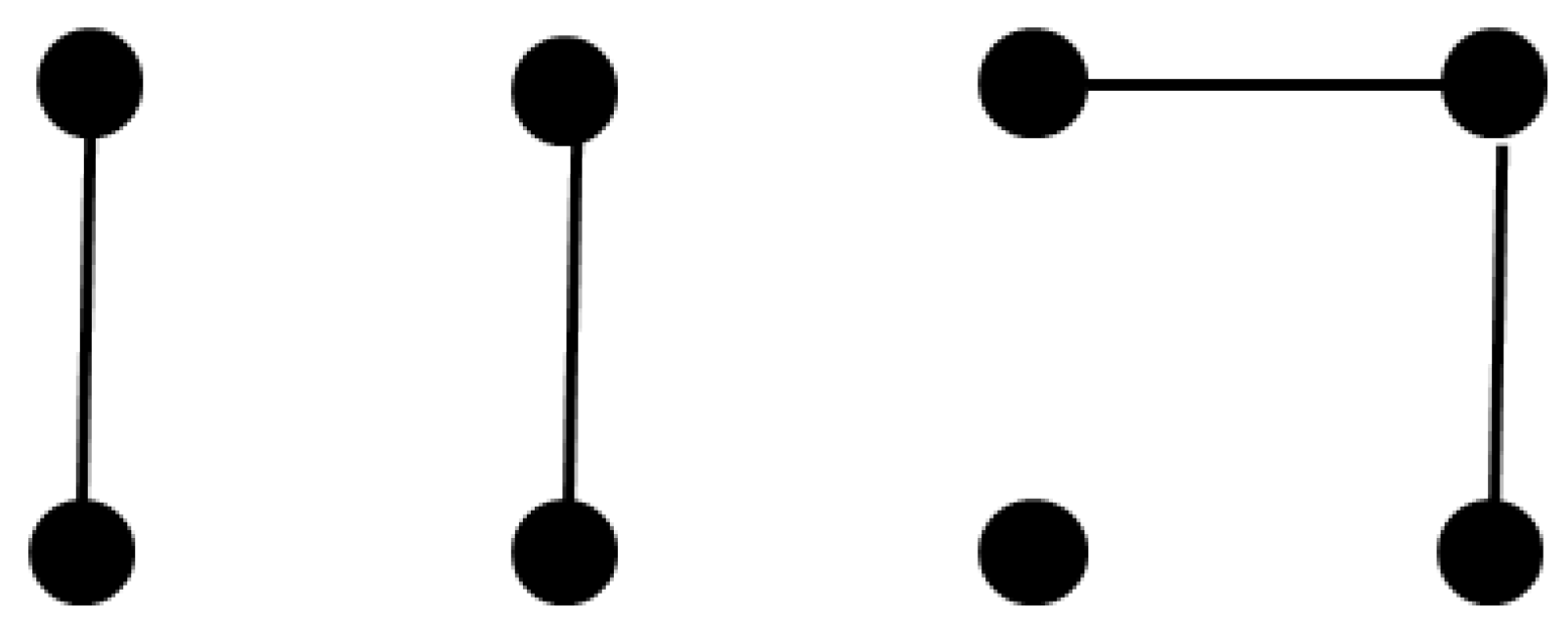
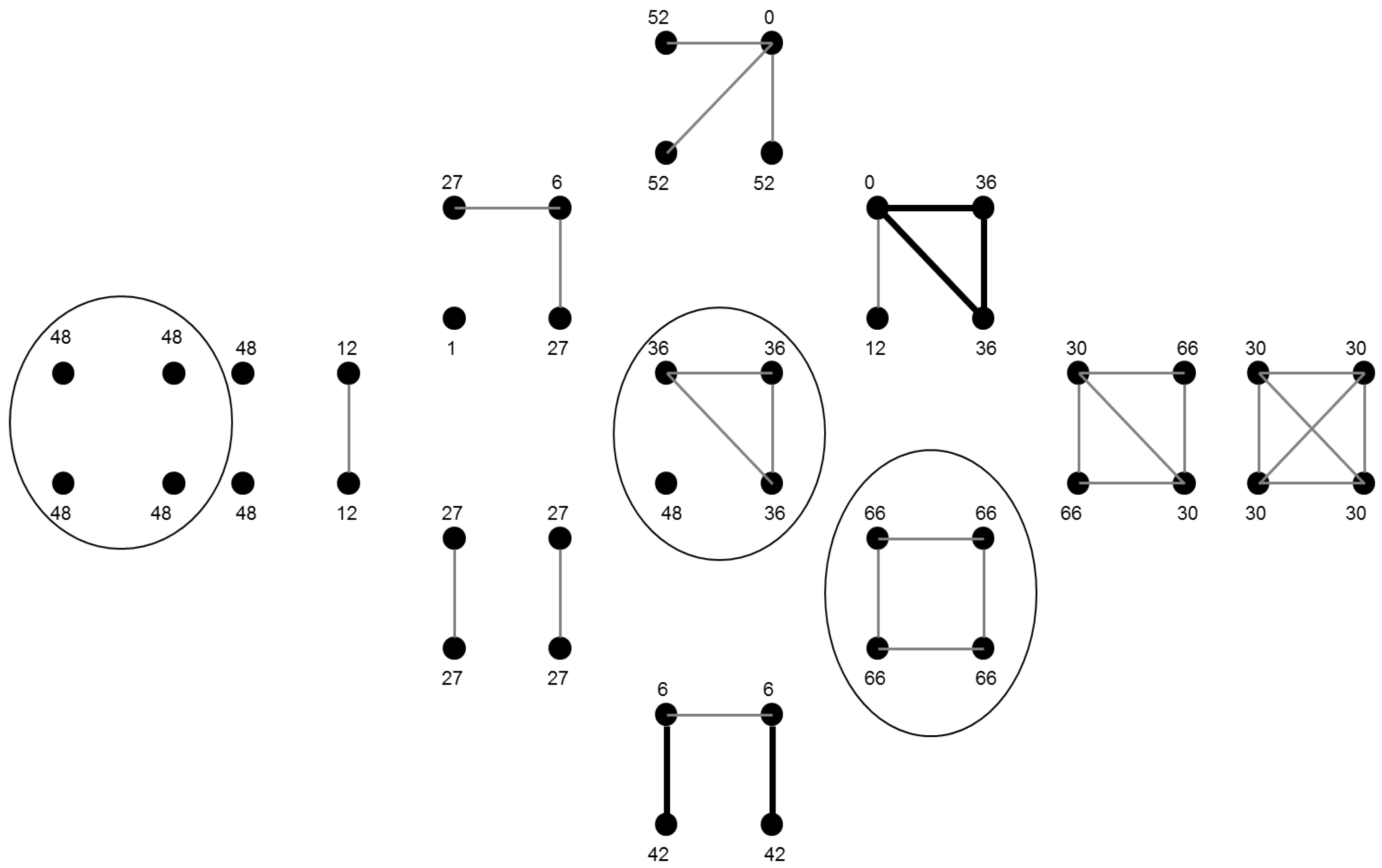
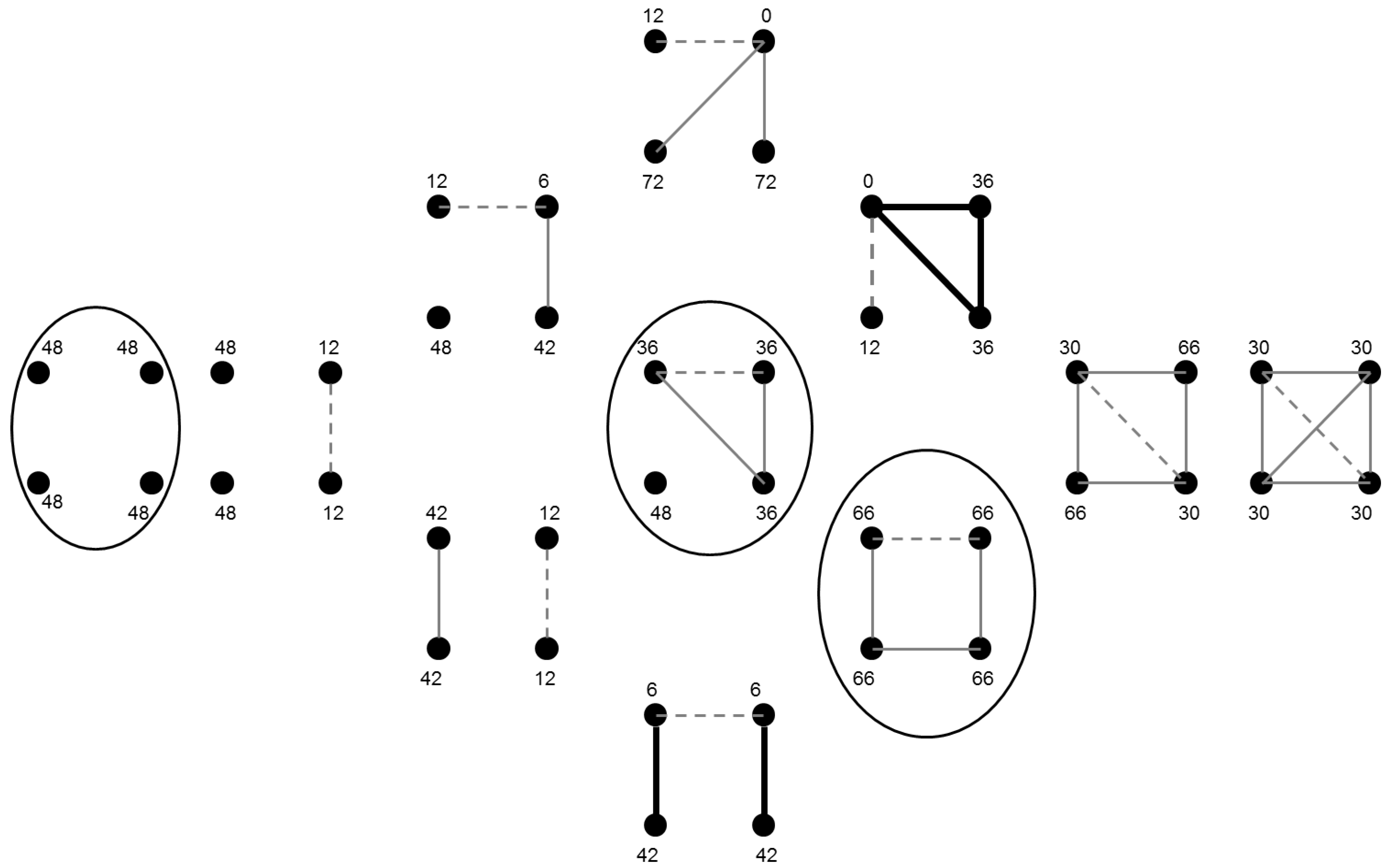
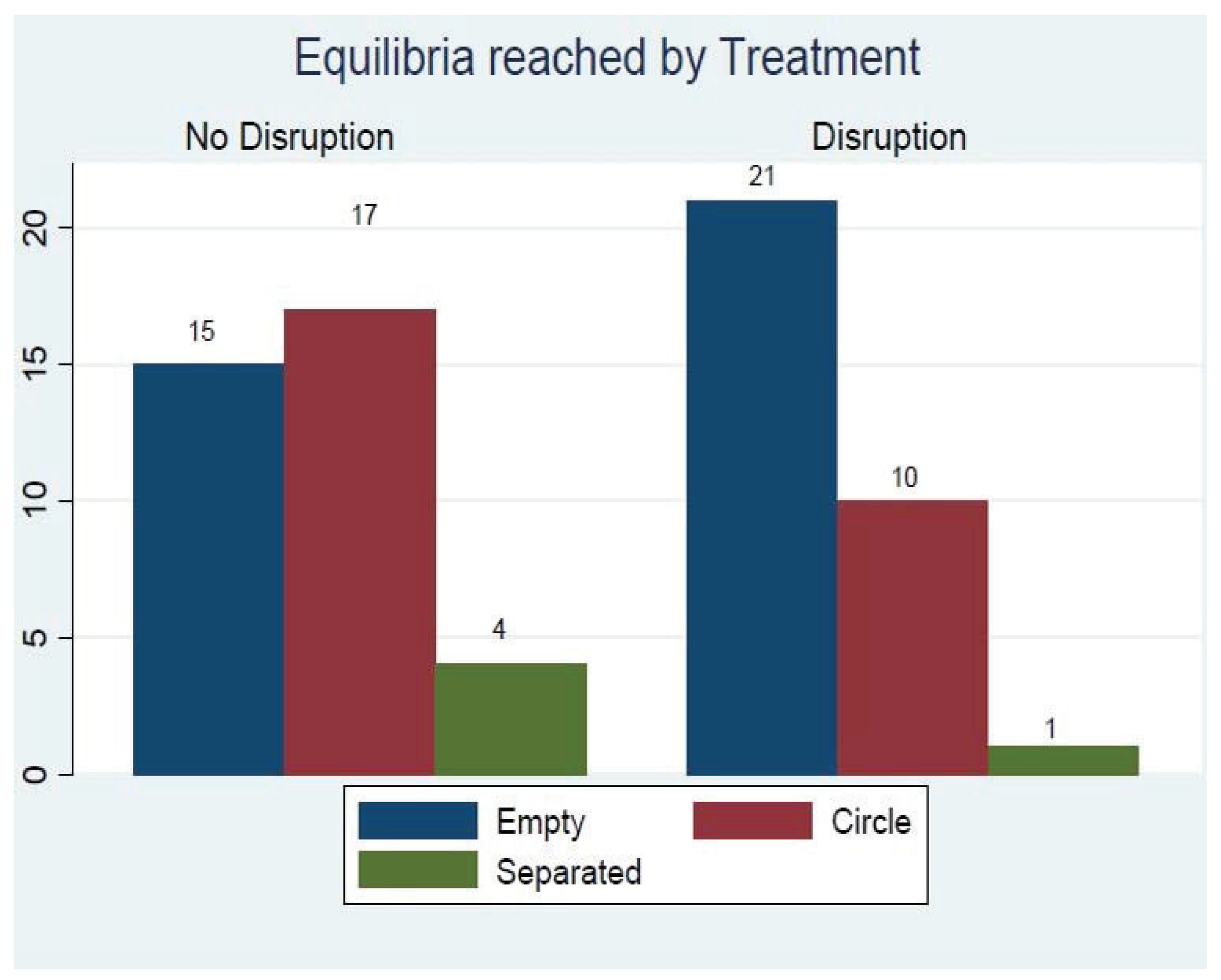
Table 1.
Summary statistics.
| Variable | Mean | Std. Dev. | Min. | Max. | N |
|---|---|---|---|---|---|
| Male | 0.473 | 0.499 | 0 | 1 | 148 |
| Age | 23.243 | 3.860 | 17 | 42 | 148 |
| Student | 0.824 | 0.381 | 0 | 1 | 148 |
| Dutch | 0.568 | 0.495 | 0 | 1 | 148 |
| Economics | 0.331 | 0.471 | 0 | 1 | 148 |
| No. of Decisions total | 11.420 | 4.408 | 2 | 22 | 148 |
| No. of Decisions R1 | 5.122 | 3.388 | 0 | 14 | 148 |
| No. of Decisions R2 | 6.297 | 3.193 | 1 | 14 | 148 |
| No. of Decisions ND | 5.311 | 3.19 | 0 | 14 | 148 |
| No. of Decisions D | 6.108 | 3.447 | 0 | 14 | 148 |
| Stop R1 | 10.243 | 6.156 | 1 | 20 | 148 |
| Stop R2 | 12.595 | 5.74 | 2 | 20 | 148 |
Table 2.
Steps of farsightedness.
| Individual | Median per Group | |||
|---|---|---|---|---|
| Number of Steps | Frequency | Percent | Frequency | Percent |
| 0 | 20 | 13.51 | 0 | 0 |
| 1 | 33 | 22.30 | 15 | 20.27 |
| 2 | 34 | 22.97 | 36 | 48.65 |
| 3 | 23 | 15.54 | 14 | 18.92 |
| 4 | 15 | 10.14 | 8 | 10.81 |
| 5 | 10 | 6.76 | 1 | 1.35 |
| 6 | 13 | 8.78 | 0 | 0 |
| Total | 148 | 100 | 74 | 100 |
Table 3.
Risk attitudes.
| Individual | Median per Group | |||
|---|---|---|---|---|
| Risk Classification | Frequency | Percent | Frequency | Percent |
| highly risk loving | 2 | 1.35 | 0 | 0 |
| very risk loving | 0 | 0 | 0 | 0 |
| risk loving | 2 | 1.35 | 0 | 0 |
| risk neutral | 23 | 15.54 | 2 | 2.70 |
| slightly risk averse | 20 | 13.51 | 6 | 8.11 |
| risk averse | 40 | 27.03 | 35 | 47.30 |
| very risk averse | 35 | 23.65 | 23 | 31.08 |
| highly risk averse | 13 | 8.78 | 8 | 10.81 |
| very highly risk averse | 13 | 8.78 | 0 | 0 |
| Total | 148 | 100 | 74 | 100 |
Table 4.
Equilibria reached.
| Frequency | Percent | |
|---|---|---|
| In Equilibrium | 65 | 87.84 |
| Not in Equilibrium | 9 | 12.16 |
| Total | 74 | 100 |
Table 5.
Equilibrium play by settings.
| Setting | Equilibrium | |||
|---|---|---|---|---|
| Starting Network | Order | Frequency | Percent | |
| line | ND-D | 17 | 94.44 | |
| line | D-ND | 13 | 81.25 | |
| dyads | ND-D | 19 | 95.00 | |
| dyads | D-ND | 19 | 95.00 | |
| Total | 68 | 91.89 | ||
*** p < 0.01, ** p < 0.05, * p < 0.1.
Table 6.
Equilibrium Play by Starting Network.
| Final Network | Starting Network Line | Starting Network Dyads | |||
|---|---|---|---|---|---|
| Frequency | Percent | Frequency | Percent | ||
| Empty | 17 | 56.67 | 19 | 50.00 | 0.0460 |
| Circle | 8 | 26.67 | 19 | 50.00 | 4.5569 ** |
| Separated | 5 | 16.66 | 0 | 0 | 6.3086 *** |
| Total | 30 | 100 | 38 | 100.00 | *** |
*** p < 0.01, ** p < 0.05, * p < 0.1.
Table 7.
Frequency of equilibria.
| Equilibrium | Frequency | Percent |
|---|---|---|
| Empty | 36 | 48.65 |
| Circle | 27 | 36.48 |
| Separated | 5 | 6.76 |
| None | 6 | 8.11 |
| Total | 74 | 100 |
Table 8.
Type of first decision in Round 1 by treatment.
| Disruption | No Disruption | ||||
|---|---|---|---|---|---|
| Frequency | Percent | Frequency | Percent | Total | |
| Myopic | 25 | 34.72 | 17 | 22.37 | 42 |
| Farsighted | 32 | 44.44 | 39 | 51.32 | 71 |
| Ambiguous | 13 | 18.06 | 20 | 26.32 | 33 |
| Irrational | 2 | 2.78 | 0 | 0 | 2 |
| Total | 72 | 100.00 | 76 | 100 | |
Table 9.
Correlations between measures of farsightedness.
| Beauty | First Dec | Revealed | |
|---|---|---|---|
| Beauty | 1.0000 | ||
| First Dec | 0.1191 | 1.0000 | |
| Revealed | 0.0496 | 0.7848 *** | 1.0000 |
*** p < 0.01, ** p < 0.05, * p < 0.1.
Table 10.
Multinomial regression on equilibria reached with the empty network as a base group.
| Circle | Separated | |||
|---|---|---|---|---|
| Coeff. | RRR | Coeff. | RRR | |
| Median of Revealed Farsighted Players Per Group | 1.909 ** | 6.743 | −2.827 | 0.059 |
| (0.897) | (2.131) | |||
| Disruption | −1.488 ** | 0.226 | −3.599 ** | 0.027 |
| (0.702) | (1.857) | |||
| Median Risk Lovingness per Group | −0.055 | 0.946 | 0.338 | 1.402 |
| (0.354) | (0.981) | |||
| Round 1 | −0.925 | 0.397 | 0.882 | 2.415 |
| (0.639) | (1.645) | |||
| Average No. of Females per Group | −0.503 | 1.654 | −1.230 | 0.292 |
| (1.099) | (2.354) | |||
| Average No. of Economics Students per Group | −1.717 | 0.179 | −3.508 | 0.029 |
| (1.429) | (3.507) | |||
| 0 Players Who Know Game Theory | 0.099 | 1.104 | 1.976 | 7.214 |
| (1.881) | (3.259) | |||
| 1 Player Who Knows Game Theory | −0.838 | 0.433 | −0.264 | 0.768 |
| (1.572) | (2.384) | |||
| 2 Players Who Know Game Theory | 0.874 | 2.396 | 16.730 | 1.84 × 10 |
| (1.389) | (1.793) | |||
| 3 Players Who Know Game Theory | 1.717 | 5.567 | 15.856 | 7.690 |
| (1.383) | (1.793) | |||
| Constant | −0.825 | - | −15.191 | - |
| (2.149) | (1.793) | |||
| Observations | 67 | 67 | ||
Standard errors in parentheses, *** p < 0.01, ** p< 0.05, * p< 0.1.
Table 11.
Equilibrium play by treatment.
| Disruption | No Disruption | |||
|---|---|---|---|---|
| Frequency | Percent | Frequency | Percent | |
| In Equilibrium | 32 | 86.50 | 36 | 97.30 |
| Not in Equilibrium | 5 | 13.50 | 1 | 2.70 |
| Total | 37 | 100 | 37 | 100 |
Table 12.
Distribution of equilibria between the circle and empty network.
| No Disruption | Disruption | ||
|---|---|---|---|
| Circle | 17 | 10 | |
| Empty | 15 | 21 | |
| Total | 32 | 31 | * |
*** p < 0.01, ** p < 0.05, * p < 0.1.
© 2018 by the authors. Licensee MDPI, Basel, Switzerland. This article is an open access article distributed under the terms and conditions of the Creative Commons Attribution (CC BY) license (http://creativecommons.org/licenses/by/4.0/).
Share and Cite
MDPI and ACS Style
Hoyer, B.; Rosenkranz, S. Determinants of Equilibrium Selection in Network Formation: An Experiment. Games 2018, 9, 89. https://0-doi-org.brum.beds.ac.uk/10.3390/g9040089
AMA Style
Hoyer B, Rosenkranz S. Determinants of Equilibrium Selection in Network Formation: An Experiment. Games. 2018; 9(4):89. https://0-doi-org.brum.beds.ac.uk/10.3390/g9040089
Chicago/Turabian StyleHoyer, Britta, and Stephanie Rosenkranz. 2018. "Determinants of Equilibrium Selection in Network Formation: An Experiment" Games 9, no. 4: 89. https://0-doi-org.brum.beds.ac.uk/10.3390/g9040089
Note that from the first issue of 2016, this journal uses article numbers instead of page numbers. See further details here.