Ergosphere, Photon Region Structure, and the Shadow of a Rotating Charged Weyl Black Hole

Abstract

In this paper, we explore the photon region and the shadow of the rotating counterpart of a static charged Weyl black hole, which has been previously discussed according to null and time-like geodesics. The rotating black hole shows strong sensitivity to the electric charge and the spin parameter, and its shadow changes from being oblate to being sharp by increasing in the spin parameter. Comparing the calculated vertical angular diameter of the shadow with that of M87*, we found that the latter may possess about ${10}^{36}$ protons as its source of electric charge, if it is a rotating charged Weyl black hole. A complete derivation of the ergosphere and the static limit is also presented.

1. Introduction

The recent black hole imaging of the shadow of M87*, performed by the Event Horizon Telescope (EHT) [1], was another significant affirmation of general relativity. Despite this, the quest for finding reliable modified and alternative theories of gravity still remains in force. This mostly stems from the modern galactic and extra-galactic evidence [2,3,4,5,6] that has led to the consideration of dark matter and dark energy scenarios. On the other hand, since these exotic cosmological constituents are extremely hard to detect, some scientists believe that increasing our knowledge about the action of the gravitational field can exclude the necessity of dark matter and dark energy scenarios in cosmological descriptions. This is pursued through finding newer gravitational actions and studying the resultant theories [7].

The exploration of these theories, however, is not done only by means of cosmological observations. In fact, as in the general relativistic cases, the possible black hole solutions inferred from modified and alternative theories of gravity are constantly investigated regarding the photon trajectories in their exterior geometry, as well as their natural optical appearance to distant observers. This latter, because of the possible relevance between the shadow of black holes and their physical characteristics, has been set to rigorous numerical and analytical studies, in order to assess the black hole solutions regarding the observations.

In addition to the efforts done for recovering the dark matter and dark energy cosmological predictions, the selection of alternative theories of gravity is also based on the peculiarities of their gravitational action. Along the same efforts, the fourth order theory of conformal gravity appeared as one of the alternatives to compare the theoretical results with the cosmological and astrophysical observations, and some considerable constraints have been driven. This theory was formulated by H. Weyl in 1918 [8], revived by Riegert in 1984 [9], and since then, has been applied widely to explain astrophysical phenomena (see, for example [10,11,12,13,14,15,16,17,18]).

It has also been argued that, unlike other cosmological models, this theory can avoid the age problem. The latter has been shown by testing the theory with the quasar APM 08279 + 5255 with the age of $(2.1\pm 0.34)\times {10}^9$ years at $z=3.91$, indicating that the theory could accommodate the quasar within a 3$\sigma$ confidence levels [19]. Furthermore, this theory has been applied to the determination of the energy carried by gravitational waves [20,21,22,23].

Based on the above notes, in this paper, we consider a black hole solution that was generated in the context of Weyl gravity. In fact, the black hole spacetimes inferred from theories of gravity are essentially constructed on the static vacuum solutions to their equations of motion. For the case of Weyl conformal gravity, such a solution was proposed by Mannheim and Kazanas in [24], where the authors connected the presence of flat galactic rotation curves to an additional effective potential available in their solution.

In this way, Weyl gravity was proposed as an alternative to dark matter. Ever since, the theory has also been intended to recover the cosmological observations related to the dark energy scenario [11,25]. Accordingly, and provided the Mannheim–Kazanas solution, the theory has been put to numerous investigations [12,13,26,27,28,29,30,31,32,33,34,35,36,37,38,39,40,41,42,43,44,45,46,47,48,49,50]. The black hole spacetime associated with this static solution, contains a cosmological term, and the rotating and electrically charged solutions to Weyl gravity have been also proposed in [51], in the context of Kerr and Kerr–Newman spacetimes.

In this work, we also consider a rotating charged black hole spacetime, inferred from Weyl gravity. This solution is indeed the rotating counterpart of a particular static charged black hole, introduced in [52]. This charged Weyl black hole (CWBH) has been recently studied regarding the light propagation in vacuum and in plasmic medium [53,54] and the motion of neutral and charged particles [55,56]. As it is a rather interesting subject to understand how a black hole would appear in an observer’s sky, it is therefore completely natural to discuss the optical properties of the rotating charged Weyl black hole (RCWBH) and its shadow. For the case of the Mannheim–Kazanas solution, a rotating version of the Weyl black hole was given in [50], and its shadow was discussed in [57].

In this paper, we follow these steps: In Section 2, we introduce the CWBH solution and apply a modified Newman–Janis method to obtain its rotating counterpart (the RCWBH), and we discuss the horizon structure. In Section 3, this solution is studied in more detail regarding the stationary and static observers, and accordingly, the ergosphere of the black hole is calculated and discussed. We use the first order light-like geodesic equations in Section 4, to proceed with studying the optical appearance of the black hole to distant observers, by means of calculating the photon region and the black hole shadow. A particular geometric method is then used to indicate the conformity between the deformation and the angular size of the shadow. We conclude in Section 5. Through the paper, we employ geometric units, in which $G=c=1$.

2. The Black Hole Solution

The gravitational action corresponding to Weyl gravity is written in terms of the Weyl conformal tensor, as

$$I_W=-\mathcal{K}\int {\mathrm{d}}^{4}x\sqrt{-g}{C}_{\alpha \beta \rho \lambda }{C}^{\alpha \beta \rho \lambda },$$

(1)

in which $\mathcal{K}$ is a coupling constant, $g=\det \left(g_{\alpha \beta }\right)$, and

$$C_{\alpha \beta \lambda \rho }=R_{\alpha \beta \lambda \rho }-\frac{1}{2}\left(g_{\alpha \lambda }{R}_{\beta \rho }-g_{\alpha \rho }{R}_{\beta \lambda }-g_{\beta \lambda }{R}_{\alpha \rho }+g_{\beta \rho }{R}_{\alpha \lambda }\right)+\frac{R}{6}\left(g_{\alpha \lambda }{g}_{\beta \rho }-g_{\alpha \rho }{g}_{\beta \lambda }\right).$$

(2)

The conformal symmetry of this theory is inferred from the fact that the action $I_W$ is invariant under the conformal transformation $g_{\alpha \beta }\left(x\right)=e^{2\alpha \left(x\right)}{g}_{\alpha \beta }\left(x\right)$, in which, $2\alpha \left(x\right)$ is termed as the local spacetime stretching. Recasting $I_W$ in the form

$$I_W=-\mathcal{K}\int {\mathrm{d}}^{4}x\sqrt{-g}\left(R^{\alpha \beta \rho \lambda }{R}_{\alpha \beta \rho \lambda }-2R^{\alpha \beta }{R}_{\alpha \beta }+\frac{1}{3}{R}^2\right),$$

(3)

it is seen that the Gauss–Bonnet term $\sqrt{-g}(R^{\alpha \beta \rho \lambda }{R}_{\alpha \beta \rho \lambda }-4R^{\alpha \beta }{R}_{\alpha \beta }+R^2)$ is a total divergence and can be disregarded. We can, therefore, simplify the action as [24,58]

$$I_W=-2\mathcal{K}\int {\mathrm{d}}^{4}x\sqrt{-g}\left(R^{\alpha \beta }{R}_{\alpha \beta }-\frac{1}{3}{R}^2\right).$$

(4)

The equations of motion are then obtained by applying the principle of least action, $\frac{\delta I_W}{\delta g_{\alpha \beta }}=0$, providing the Bach equation

$$\begin{array}{ccc}\hfill W_{\alpha \beta }& =& {\mathfrak{P}}_{\gamma \delta }{{{C_{\alpha }}^{\gamma }}_{\beta }}^{\delta }+\square {\mathfrak{P}}_{\alpha \beta }-{\nabla }^{\gamma }{\nabla }_{\alpha }{\mathfrak{P}}_{\beta \gamma }\hfill \\ & =& \frac{1}{4\mathcal{K}}{T}_{\alpha \beta },\hfill \end{array}$$

(5)

in which $W_{\alpha \beta }$ is the trace-less Bach tensor, $\square \equiv {\nabla }^{\gamma }{\nabla }_{\gamma }$, and

$${\mathfrak{P}}_{\alpha \beta }=\frac{1}{2}\left(R_{\alpha \beta }-\frac{1}{4}{g}_{\alpha \beta }R\right),$$

(6)

is the Schouten tensor, which is expressed in terms of the Ricci tensor and the scalar curvature of the spacetime. For a vanishing energy–momentum tensor ($T_{\alpha \beta }=0$), the Mannheim–Kazanas static spherically symmetric solution is given by the metric

$$\mathrm{d}{s}^2=-B\left(r\right)\mathrm{d}{t}^2+\frac{\mathrm{d}{r}^2}{B\left(r\right)}+r^2(\mathrm{d}{\theta }^2+{\sin }^2\theta \mathrm{d}{\varphi }^2)$$

(7)

in the usual Schwarzschild coordinates ($-\infty <t<\infty$, $r\ge 0$, $0\le \theta \le \pi$ and $0\le \varphi \le 2\pi$), with the lapse function [24]

$$B\left(r\right)=1-\frac{\zeta \left(2-3\zeta \rho \right)}{r}-3\zeta \rho +\rho r-\sigma r^2.$$

(8)

The three-dimensional integration constants $\zeta$, $\rho$, and $\sigma$, help in recovering the general relativistic black hole spacetimes, in the way that for $\rho \to 0$, the Schwarzschild–de Sitter solution is recovered. This corresponds to distances much smaller than $1/\rho$.

In the case that the energy–momentum tensor is associated with the electrostatic vector potential

$$A_{\alpha }=\left(\frac{q}{r},0,0,0\right),$$

(9)

for a spherically symmetric massive source of electric charge q, in [52], the vacuum Bach equation (i.e., $W_{\alpha \beta }=0$ in Equation (5)) is solved for the reference lapse function

$$B\left(r\right)=1-\frac{2\mathrm{C}}{r}-\frac{1}{3}f\left(r\right),$$

(10)

which provides the simple solution

$$f\left(r\right)=-\left(\frac{6\mathrm{C}}{r}+c_1{r}^2+c_{2}r\right),$$

(11)

for which, substitution in Equation (10), yields

$$B\left(r\right)=1+\frac{1}{3}\left(c_{2}r+c_1{r}^2\right).$$

(12)

The determination of the coefficients $c_1$ and $c_2$ in the above lapse function is done through the weak-field limit approach, by considering the last two terms of $B\left(r\right)$ as perturbations on the Minkowski spacetime [35,52]. In this way, by taking into account a spherically symmetric source of mass $\tilde{m}$, charge $\tilde{q}$ and radius $\tilde{r}$, the Poisson equation ${\nabla }^2{h}_{\alpha \beta }=8\pi T_{\alpha \beta }$, with $h_{\alpha \beta }=g_{\alpha \beta }-{\eta }_{\alpha \beta }$, has the following 00 component in Minkowski spacetime:

$${\nabla }^2{h}_{00}\equiv -\frac{1}{3}\left(\frac{{\partial }^2}{\partial r^2}+\frac{2}{r}\frac{\partial }{\partial r}\right)\left(c_1{r}^2+c_{2}r\right)=8\pi T_{00}=8\pi \left(\frac{\tilde{m}}{\frac{4}{3}\pi {\tilde{r}}^3}+\frac{1}{8\pi }\frac{{\tilde{q}}^2}{r^4}\right),$$

(13)

in which, $T_{00}$ is the scalar part of the total energy–momentum tensor, which corresponds to the mass and charge of the source. From Equation (13), we obtain the relation [52]

$$c_2=-\left(\frac{9\tilde{m}r}{{\tilde{r}}^3}+\frac{3}{2}\frac{{\tilde{q}}^2}{r^3}+3c_{1}r\right),$$

(14)

which provides

$$B\left(r\right)=1-\frac{r^2}{{\lambda }^2}-\frac{Q^2}{4r^2},$$

(15)

where

$$\begin{array}{ccc}& & \frac{1}{{\lambda }^2}=\frac{3\tilde{m}}{{\tilde{r}}^3}+\frac{2\tilde{\epsilon }}{3},\hfill \end{array}$$

(16)

$$\begin{array}{ccc}& & Q=\sqrt{2}\tilde{q}.\hfill \end{array}$$

(17)

The coefficient $\tilde{\epsilon }\equiv c_1$ in Equation (16), is intended to recover the cosmological constituents of the spacetime and, here, has the dimension of ${\mathrm{m}}^{-2}$. Accordingly, the lapse function (15) provides the exterior geometry of the CWBH. In the adopted geometric system of units, Q and $\lambda$ have the dimensions of $\mathrm{m}$. For $\lambda >Q$, this spacetime allows for two horizons; an event horizon ${\mathrm{r}}_{+}$, and a cosmological horizon ${\mathrm{r}}_{++}$ (instead of a Cauchy horizon), given by [55]

$$\begin{array}{ccc}& & {\mathrm{r}}_{+}=\lambda \sin \left(\frac{1}{2}\arcsin \left(\frac{Q}{\lambda }\right)\right),\hfill \end{array}$$

(18)

$$\begin{array}{ccc}& & {\mathrm{r}}_{++}=\lambda \cos \left(\frac{1}{2}\arcsin \left(\frac{Q}{\lambda }\right)\right).\hfill \end{array}$$

(19)

The extremal CWBH is obtained for $\lambda =Q$, whose causal structure is characterized by the unique horizon ${\mathrm{r}}_{\mathrm{ex}}={\mathrm{r}}_{+}={\mathrm{r}}_{++}=\lambda /\sqrt{2}$. The case of $\lambda <Q$, then, corresponds to a naked singularity. To reduce the CWBH to the Reissner–Nordström-(Anti–)de Sitter black hole of mass $M_0$, charge $Q_0$, and cosmological constant $\Lambda$, we need to let $\tilde{r}$ be a free radial distance, $3\tilde{m}\to M_0$, $2\tilde{\epsilon }\to \pm \Lambda$, and $Q\to 2i{Q}_0$ (an imaginary transformation).

The Rotating Counterpart

To obtain the rotating counterpart of the CWBH, we tend to recast the CWBH solution in a stationary non-static form in the Boyer–Lindquist coordinates. Such transformations are commonly done through the Newman–Janis algorithm of complexification of the radial coordinate [59]. This method has been widely used to generate stationary black hole solutions from their static counterparts1. At first, this algorithm was intended to generate the Kerr solution from the Schwarzschild spacetime, and therefore was developed in the context of general relativity. It however, has had recent applications to black hole solutions in alternative theories of gravity [61,62,63,64].

On the other hand, it has been indicated that, when applied to alternative gravity, this method leads to distortions in the resultant rotating spacetimes by introducing extra unknown sources into the original source [65]. Hence, to obtain the rotating counterpart of the CWBH spacetime, we applied the method proposed by Azreg-Aïnou in [66,67], which is the modified version of the Newman–Janis algorithm and has been applied successfully in producing imperfect rotating solutions from their static counterparts. Employing this method for the line element (7), we obtain the following rotating spacetime:

$$\mathrm{d}{s}^2=-\frac{\Xi }{\Sigma }\mathrm{d}{t}^2+\frac{\Sigma }{\Delta }\mathrm{d}{r}^2+\Sigma \mathrm{d}{\theta }^2-2a{\sin }^2\theta \left(1-\frac{\Xi }{\Sigma }\right)\mathrm{d}t\mathrm{d}\varphi +{\sin }^2\theta \left[\Sigma +a^2{\sin }^2\theta \left(2-\frac{\Xi }{\Sigma }\right)\right]\mathrm{d}{\varphi }^2,$$

(20)

where

$$\begin{array}{cc}\hfill & \Xi =\Delta -a^2{\sin }^2\theta ,\hfill \end{array}$$

(21a)

$$\begin{array}{cc}\hfill & \Delta =a^2+r^{2}B\left(r\right),\hfill \end{array}$$

(21b)

$$\begin{array}{cc}\hfill & \Sigma =r^2+a^2{\cos }^2\theta ,\hfill \end{array}$$

(21c)

in which, a is the black hole’s spin parameter, defined as $a=J/\tilde{m}$, with J as the black hole’s angular momentum. Therefore, a has the dimension of $\mathrm{m}$ in our geometric units. The black hole’s angular velocity is $\omega =-g_{t\varphi }/g_{\varphi \varphi }$ [68]. In fact, if the reference lapse function (10) is applied to Equation (21b), the components of the Bach tensor $W_{\alpha \beta }$, are vanished for the same expression of $f\left(r\right)$ as those in Equation (11).

We must, however, note that this process can only be done by substitution of this lapse function in the components of the Bach tensor by applying computer software2. Hence, the line element (20) is a vacuum rotating solution to Weyl gravity, if a lapse function of the general form (12) is taken into account. Accordingly, for a massive charged spherical source, like the one assumed for the CWBH, the same constants can be obtained if the same method is pursued. The only difference is that, the associated vector potential generated by the source, changes in its form from that in Equation (9), to [69]

$${\tilde{A}}_{\alpha }=\frac{qr}{\Sigma }\left(1,0,0,-a{\sin }^2\theta \right).$$

(22)

The exterior geometry of the RCWBH is, therefore, specified by applying the lapse function (15), which provides

$$\Delta =a^2+r^2-\frac{r^4}{{\lambda }^2}-\frac{Q^2}{4}.$$

(23)

As for the spherically symmetric stationary spacetimes, the RCWBH admits two Killing vectors, ${\mathbf{\xi }}_{\left(t\right)}$ and ${\mathbf{\xi }}_{\left(\varphi \right)}$, satisfying

$$\begin{array}{ccc}\hfill & & {\xi }_{\left(t\right)}^{\alpha }{\xi }_{\alpha \left(t\right)}=g_{tt},\hfill \end{array}$$

(24)

$$\begin{array}{ccc}& & {\xi }_{\left(\varphi \right)}^{\alpha }{\xi }_{\alpha \left(\varphi \right)}=g_{\varphi \varphi },\hfill \end{array}$$

(25)

which correspond to the translational and rotational symmetries and the relevant invariants of motion. The black hole’s event and cosmological horizons are now obtained by solving $g^{rr}=0$, which results in (see Appendix A)

$$\begin{array}{ccc}\hfill & & r_{+}=\lambda \sin \left(\frac{1}{2}\arcsin \left(\frac{2}{\lambda }\sqrt{\frac{Q^2}{4}-a^2}\right)\right),\hfill \end{array}$$

(26)

$$\begin{array}{ccc}& & r_{++}=\lambda \cos \left(\frac{1}{2}\arcsin \left(\frac{2}{\lambda }\sqrt{\frac{Q^2}{4}-a^2}\right)\right),\hfill \end{array}$$

(27)

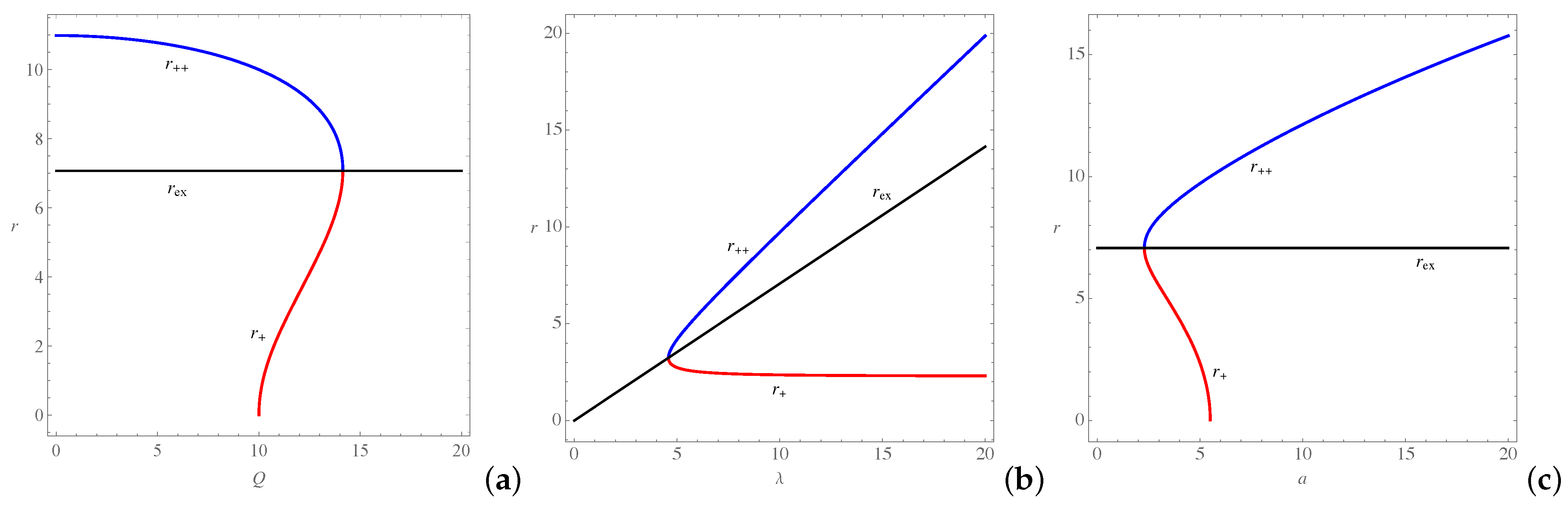
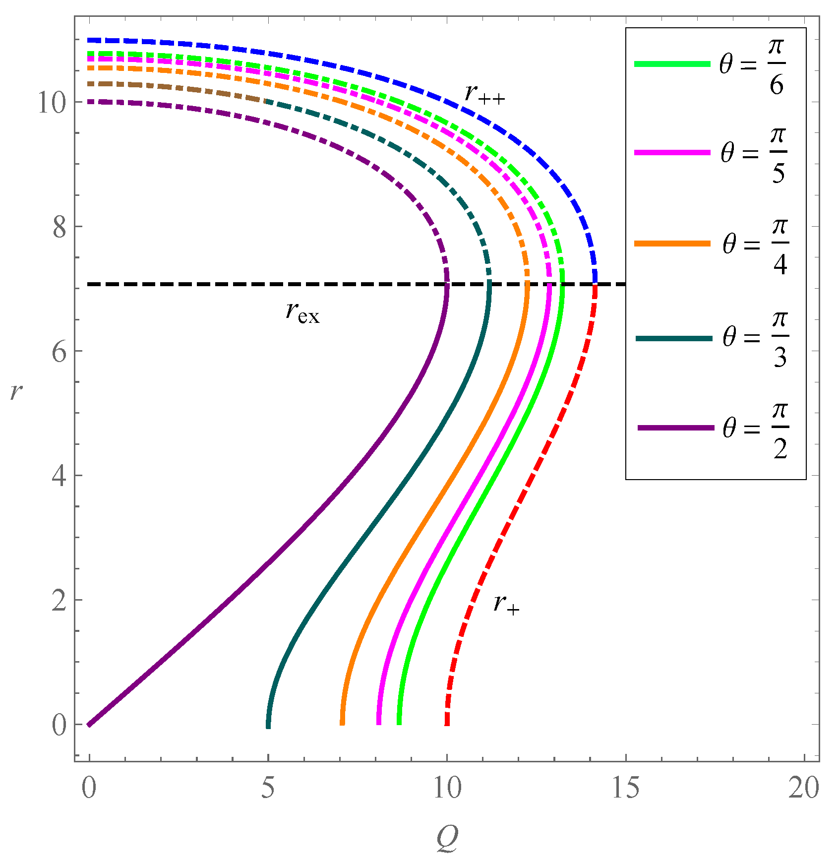
for which the extremal black hole horizon $r_{\mathrm{ex}}=\lambda /\sqrt{2}$ is obtained for $Q_{\mathrm{ex}}=\pm \sqrt{4a^2+{\lambda }^2}$, and a naked singularity appears for $Q>\sqrt{4a^2+{\lambda }^2}$ (for $Q>0$). As shown in Figure 1, not all values of Q, $\lambda$ and a are allowed to construct a black hole (censored region). As shown in Figure 2, for fixed $\lambda$ and a, increases in Q increase the size of $r_{+}$ and decrease that of $r_{++}$, until they coincide on $r_{+}=r_{++}=r_{\mathrm{ex}}$ at $Q=Q_{\mathrm{ex}}$. The same happens for a decrease in $\lambda$ for fixed Q and a, which leads to $\lambda ={\lambda }_{\mathrm{ex}}$, and a decrease in a for fixed $\lambda$ and Q, leading to $a=a_{\mathrm{ex}}$. It is also easy to show that the hypersurfaces corresponding to $r_{+}$ and $r_{++}$, are null. We continued analyzing the RCWBH in the next section, regarding the stationary and static observers.

3. The Ergosphere

In addition to being encompassed by the event horizon, the rotating black holes are also characterized by another hypersurface, which is formed as a result of the black hole’s spin and limits the existence of static observers. This surface is, therefore, identified with the event horizon only in the limit of the vanishing spin parameter [70,71,72]. In this section, we determine this surface and discuss it analytically as well as illustratively. However, let us first consider an important feature of rotating spacetimes, by considering the zero angular momentum observers (ZAMOs) with the vanishing angular momentum defined as [68]

$$\begin{array}{ccc}\hfill \tilde{L}& \equiv & g_{\varphi \alpha }{\frac{\mathrm{d}x}{\mathrm{d}\tau }}^{\alpha }\hfill \\ & =& g_{\varphi t}\frac{\mathrm{d}t}{\mathrm{d}\tau }+g_{\varphi \varphi }\frac{\mathrm{d}\varphi }{\mathrm{d}\tau }=0,\hfill \end{array}$$

(28)

in which $\tau$ is the proper time associated with the observers (or particles) and, throughout this paper, we assign it to the trajectory parameter. Accordingly, the observer’s angular velocity is obtained from Equations (20) and (21), reading as

$$\Omega =\frac{\mathrm{d}\varphi }{\mathrm{d}t}=-\frac{g_{t\varphi }}{g_{\varphi \varphi }}=\frac{a\left(r^2+a^2-\Delta \right)}{{\left(r^2+a^2\right)}^2-\Delta a^2{\sin }^2\theta },$$

(29)

which is the same as the angular velocity of the rotating black hole and increases as r decreases, until it reaches its maximum value

$${\Omega }_{max}{=\Omega |}_{r=r_{+}}\equiv {\Omega }_H=\frac{a}{r_{+}^2+a^2}={\omega }_{+},$$

(30)

where ${\omega }_{+}\equiv \omega \left(r_{+}\right)$ is the black hole’s angular velocity at its event horizon. For a slowly rotating black hole (small a), ${\Omega }_H$ reduces to

$${\Omega }_H\approx \frac{a}{{\lambda }^2{\sin }^2\left(\frac{1}{2}\arcsin \left(\frac{Q}{\lambda }\right)\right)}.$$

(31)

Therefore, on the event horizon, ZAMOs move in the same direction as the black hole’s own rotation (also called corotation), as a result of dragging their inertial frames. Aside from the ZAMOs, to deal with the static observers, let us consider their velocity four-vector as

$$u^{\alpha }=\mathfrak{n}{\xi }_{\left(t\right)}^{\alpha },$$

(32)

with the normalization factor $\mathfrak{n}={(-g_{\alpha \beta }{\xi }_{\left(t\right)}^{\alpha }{\xi }_{\left(t\right)}^{\beta })}^{-1/2}=1/\sqrt{-g_{tt}}$, according to Equation (24). Such observers cannot exist everywhere in the spacetime, and they are confined to a limit defined in terms of the validity of Equation (32). In fact, for ${\mathfrak{n}}^{-2}=-g_{tt}=0$, this equation breaks down, and ${\mathbf{\xi }}_{\left(t\right)}$ becomes null. In this way, a static limit3 is obtained, whose radius, $r_{SL}$, is calculated by solving the equation $g_{tt}=0$. This equation yields the two positive solutions

$$\begin{array}{ccc}\hfill & & r_{SL1}=\lambda \sin \left(\frac{1}{2}\arcsin \left(\frac{2}{\lambda }\sqrt{\frac{Q^2}{4}-a^2{\cos }^2\theta }\right)\right),\hfill \end{array}$$

(33)

$$\begin{array}{ccc}& & r_{SL2}=\lambda \cos \left(\frac{1}{2}\arcsin \left(\frac{2}{\lambda }\sqrt{\frac{Q^2}{4}-a^2{\cos }^2\theta }\right)\right),\hfill \end{array}$$

(34)

that satisfy the condition of causality $r_{+}<r_{SL1}<r_{SL2}<r_{++}$. The domain $r<r_{SL1}$ corresponds to a region in which the static observers can no longer remain static4, and the so-called frame-dragging effect forces them to rotate with the black hole. In Figure 3, the behavior of the above two solutions was plotted for a definite value of a.

As the angular parameter increases, the static limit surface (corresponding to $r_{SL1}$) recedes from the event horizon, and hence the ergosphere expands. On the other hand, $r_{SL2}$ shrinks under the same conditions. Note that, in the case of an extremal black hole ($Q^2=4a^2+{\lambda }^2$), the above surfaces coincide at

$$r_{SL\left(\mathrm{ex}\right)}=\lambda \cos \left(\frac{\pi }{4}-\frac{1}{4}\arccos \left(\frac{8a^2{\sin }^2\theta +{\lambda }^2}{{\lambda }^2}\right)\right).$$

(35)

Comparing Equations (26) and (33), we notice that, for $\theta \ne n\pi (n=0,\pm 1,\pm 2,\dots )$, the surface of static limits does not coincide with that of the event horizon, and these surfaces, together, form an ergosphere (or ergoregion). To demonstrate the ergosphere of the black hole, let us introduce the Cartesian coordinates [74]

$$\begin{array}{cc}\hfill & x=\sqrt{r^2+a^2}\sin \theta \cos \varphi ,\hfill \end{array}$$

(36a)

$$\begin{array}{cc}\hfill & y=\sqrt{r^2+a^2}\sin \theta \sin \varphi ,\hfill \end{array}$$

(36b)

$$\begin{array}{cc}\hfill & z=r\cos \theta ,\hfill \end{array}$$

(36c)

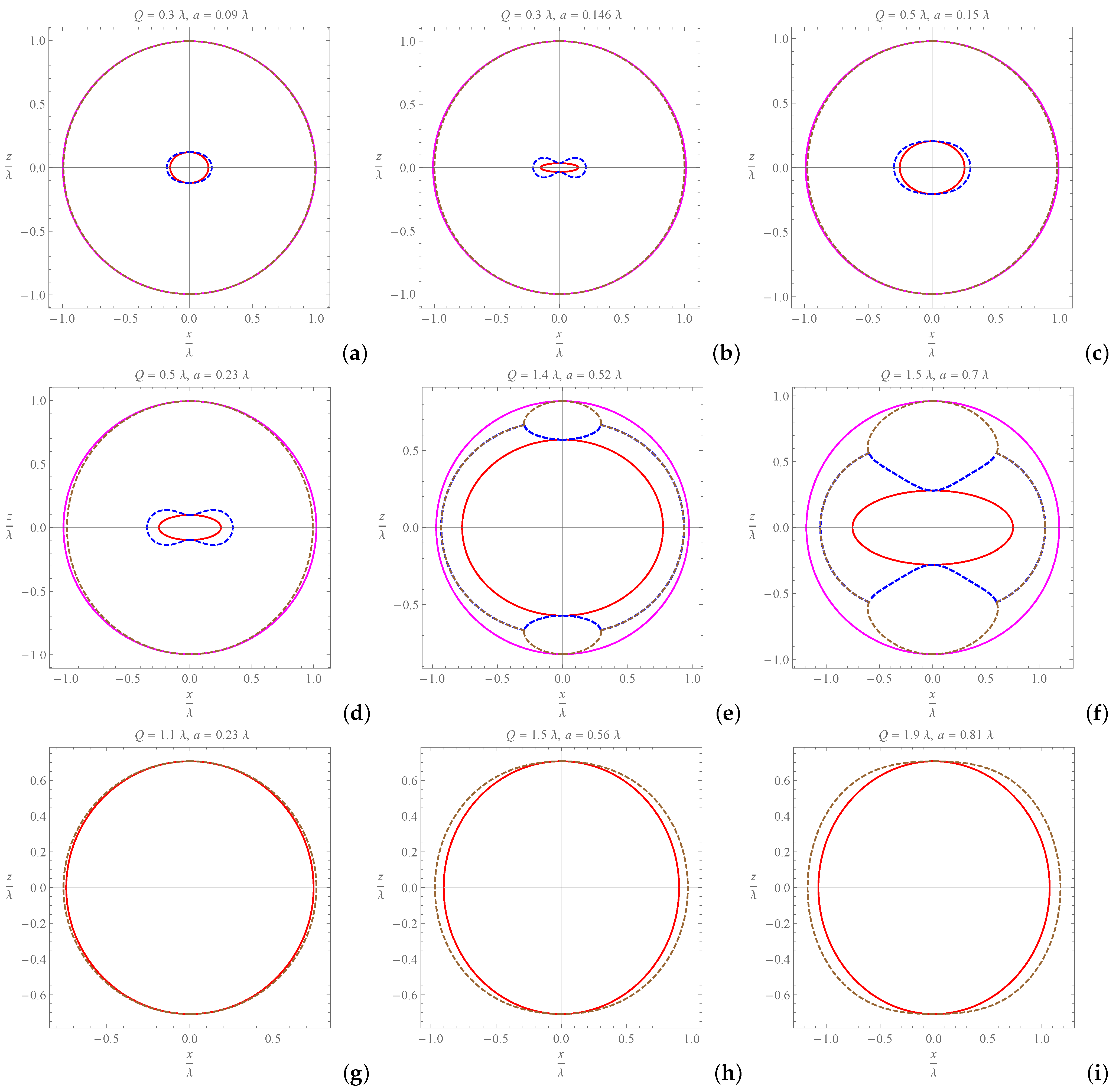
which are defined in terms of the Boyer–Lindquist coordinates of the line element (20). Accordingly, the horizon hypersurfaces can be plotted, as being observed either from the coordinate of axial symmetry (i.e., in the x-y plane), or from the y (or x) coordinate (i.e., in the z-x (or z-y) plane). In Figure 4, the horizons and the static limit surfaces are plotted for several values of a and Q within the allowed values of Figure 1, and therefore, the ergosphere for each of these cases is demonstrated.

As is seen in the figures, increases in a for each fixed value of Q stretch the event horizon’s cross-section and act in favor of dividing the ergosphere into separate regions at each side of the event horizon. In the special cases of $Q>\lambda$, $r_{SL1}$ and $r_{SL2}$ match in certain regions outside the event horizon and form ergospheres of peculiar shapes. For the extremal black hole, it is naturally $Q>\lambda$, the spacetime encounters one horizon and one static limit, and its ergosphere increases in size as the distance between the values of Q and a increases. Stationary observers of angular velocity $\Omega$ and the four-velocity $u_s^{\alpha }={\mathfrak{n}}_s{\xi }_s^{\alpha }$, with

$$\begin{array}{ccc}\hfill & & {\xi }_s^{\alpha }={\xi }_{\left(t\right)}^{\alpha }+\Omega {\xi }_{\left(\varphi \right)}^a,\hfill \end{array}$$

(37)

$$\begin{array}{ccc}& & {\mathfrak{n}}_s^{-2}=-g_{\alpha \beta }{\xi }_s^{\alpha }{\xi }_s^{\beta }=-g_{\varphi \varphi }\left({\Omega }^2-2\omega \Omega +\frac{g_{tt}}{g_{\varphi \varphi }}\right),\hfill \end{array}$$

(38)

can exist in the ergosphere, as long as the Killing vector ${\mathbf{\xi }}_s$ remains time-like. This corresponds to ${\mathfrak{n}}_s^{-2}>0$, or ${\Omega }_{-}<\Omega <{\Omega }_{+}$, with

$${\Omega }_{\pm }=\omega \pm \frac{\sqrt{\Delta }\sin \theta }{g_{\varphi \varphi }}.$$

(39)

Accordingly, this vector becomes null on the event horizon5. Therefore, by approaching the event horizon, $\Omega \to {\Omega }_H\equiv {\Omega }_{+}$, and the particles will be in the state of corotation with the black hole. Such particles encounter the surface gravity [68]

$$\kappa ={\left.\frac{{\Delta }^{\prime }\left(r\right)}{2(r^2+a^2)}\right|}_{r=r_{+}},$$

(40)

at the vicinity of the event horizon. Applying Equations (21b) and (26), and after a little algebra, this gives

$$\kappa =\frac{r_{+}}{a^2+r_{+}^2}\sqrt{{\lambda }^2-Q^2+4a^2}.$$

(41)

For the extremal black hole ($r_{+}\to r_{\mathrm{ex}}$), we have, from Equation (40), that ${\kappa }_{\mathrm{ex}}=0$. For asymptotically flat spacetimes, where the energy can be defined relative to an observer located at infinity, the ergosphere is highlighted also by a theoretical scenario, termed as the Penrose process, through which, particles of negative-energy created in the ergosphere can extract positive rotational energy from a rotating black hole [75].

The optical appearance of a black hole to distant observers does not rely on the positioning of its ergosphere, since this latter affects only the time-like particles. The conceived image of a black hole is a shadow that is confined by particular photons on unstable (critical) orbits. Such photons construct a photon surface around the black hole. For the case of the RCWBH, this will be given a detailed discussion in the next section.

4. Shadow of the Black Hole

The light propagation around black holes is of remarkable importance in astrophysics, particularly due to the evidence that can be achieved by advancements in the field of observational astronomy. Photons that lie on unstable orbits in the gravitational field of the black holes will either fall onto the event horizon or escape to infinity. To the observer, these latter ones constitute a bright photon ring that confines the black hole shadow [71,76,77,78].

In particular, the Luminet’s optical simulation of a Schwarzschild black hole and its accretion in 1979 [78] provided more insights about the photon rings resulting from the extremely warped region around the black holes. The formulations obtained in this way helped scientists to confine the shadow of rotating black holes inside their respected photon rings. Accordingly, the mathematical methods to calculate the form and size of a Kerr black hole shadow were then developed by Bardeen [70,71,79], and the same methods were reused by Chandrasekhar [72].

These methods were later developed and generalized widely (see [80,81,82,83,84,85]). Having these methods in hand, a large number of black hole spacetimes, including those with cosmological components, were given rigorous analytical calculations, simulations, numerical, and observational studies [86,87,88,89,90,91,92,93,94,95,96,97,98,99,100]. The black hole shadow is of great importance as it provides information about the light propagation in near-horizon regions. Recently, several investigations have been devoted to establish relations between the shadow and black hole parameters (see for example [101,102] for thermodynamic, and [103,104,105,106,107,108,109,110] for dynamical aspects of rotating black holes).

Here, we apply the method of separation of variables in the Hamilton–Jacobi equation [72,111]. Accordingly, we write the Hamilton–Jacobi equation as

$$\mathcal{H}=-\frac{\partial \mathcal{S}}{\partial \tau }=\frac{1}{2}{g}^{\alpha \beta }\frac{\partial \mathcal{S}}{\partial x^{\alpha }}\frac{\partial \mathcal{S}}{\partial x^{\beta }}=-\frac{1}{2}{\mu }^2,$$

(42)

where $\mathcal{H}$, $\mathcal{S}$, and $\mu$, are, respectively, the canonical Hamiltonian, the Jacobi action, and the remaining mass of particles. Defining the four-momentum $p_{\alpha }=\partial \mathcal{S}/\partial x^{\alpha }$ ($p_{\alpha }{p}^{\alpha }={\mu }^2$), the action can be separated using Carter’s method, as

$$\mathcal{S}=\frac{1}{2}{\mu }^2\tau -\tilde{\mathcal{E}}t+\tilde{\mathcal{L}}\varphi +{\mathcal{S}}_r\left(r\right)+{\mathcal{S}}_{\theta }\left(\theta \right),$$

(43)

in which ${\mathcal{S}}_r\left(r\right)\equiv p_r$, ${\mathcal{S}}_{\theta }\left(\theta \right)\equiv p_{\theta }$, and

$$\begin{array}{ccc}\hfill & & \tilde{\mathcal{E}}=-p_t=-\left(g_{tt}\frac{\mathrm{d}t}{\mathrm{d}\tau }+g_{t\varphi }\frac{\mathrm{d}\varphi }{\mathrm{d}\tau }\right),\hfill \end{array}$$

(44)

$$\begin{array}{ccc}& & \tilde{\mathcal{L}}=p_{\varphi }=g_{\varphi t}\frac{\mathrm{d}t}{\mathrm{d}\tau }+g_{\varphi \varphi }\frac{\mathrm{d}\varphi }{\mathrm{d}\tau },\hfill \end{array}$$

(45)

are the constants of motion. Physically, $\tilde{\mathcal{L}}$ is associated with the particles’ angular momentum around the axis of symmetry. On the other hand, $\tilde{\mathcal{E}}$ cannot be regarded as the energy of particles, because the spacetime under consideration is not asymptotically flat. Using Equations (43)–(45) in the Hamilton–Jacobi equation (42), and applying the method of the separation of variables for the case of mass-less particles (photons with $\mu =0$), the equations of motion are then given in terms of the four differential equations [72]

$$\begin{array}{ccc}\hfill & & \Sigma \frac{\mathrm{d}t}{\mathrm{d}\tau }=\frac{r^2+a^2}{\Delta }\left(\tilde{\mathcal{E}}\left(r^2+a^2\right)-a\tilde{\mathcal{L}}\right)-a\left(a\tilde{\mathcal{E}}{\sin }^2\theta -\tilde{\mathcal{L}}\right),\hfill \end{array}$$

(46)

$$\begin{array}{ccc}& & \Sigma \frac{\mathrm{d}r}{\mathrm{d}\tau }=\pm \sqrt{\mathcal{R}\left(r\right)},\hfill \end{array}$$

(47)

$$\begin{array}{ccc}& & \Sigma \frac{\mathrm{d}\theta }{\mathrm{d}\tau }=\pm \sqrt{\Theta \left(\theta \right)},\hfill \end{array}$$

(48)

$$\begin{array}{ccc}& & \Sigma \frac{\mathrm{d}\varphi }{\mathrm{d}\tau }=\frac{a}{\Delta }\left(\tilde{\mathcal{E}}\left(r^2+a^2\right)-a\tilde{\mathcal{L}}\right)-\left(a\tilde{\mathcal{E}}-\frac{\tilde{\mathcal{L}}}{{\sin }^2\theta }\right),\hfill \end{array}$$

(49)

defining

$$\begin{array}{cc}\hfill & \mathcal{R}\left(r\right)={\left(\left(r^2+a^2\right)\tilde{\mathcal{E}}-a\tilde{\mathcal{L}}\right)}^2-\Delta \left(\mathcal{D}+{\left(a\tilde{\mathcal{E}}-\tilde{\mathcal{L}}\right)}^2\right),\hfill \end{array}$$

(50a)

$$\begin{array}{cc}\hfill & \Theta \left(\theta \right)=\mathcal{D}-\left(\frac{{\tilde{\mathcal{L}}}^2}{{\sin }^2\theta }-a^2{\tilde{\mathcal{E}}}^2\right){\cos }^2\theta ,\hfill \end{array}$$

(50b)

in which $\mathcal{D}$ is the Carter separation constant. The photon trajectories are, therefore, characterized by two dimension-less impact parameters

$$\begin{array}{ccc}\hfill & & \tilde{b}=\frac{\tilde{\mathcal{L}}}{\tilde{\mathcal{E}}},\hfill \end{array}$$

(51)

$$\begin{array}{ccc}& & \tilde{\eta }=\frac{\mathcal{D}}{{\tilde{\mathcal{E}}}^2}.\hfill \end{array}$$

(52)

It is also common to use the generalized Carter’s constant of motion $\mathcal{K}=\mathcal{D}+{(a\tilde{\mathcal{E}}-\tilde{\mathcal{L}})}^2$ [72]. As stated before, photon surfaces are those regions around the black hole in which the photons travel on unstable (critical) orbits. In this situation, the radial effective potential associated with the photon trajectories reaches its extremum at the corresponding critical distance $r_p$. Accordingly, Equation (47) provides the conditions

$$\begin{array}{cc}\hfill & \mathcal{R}\left(r_p\right)=0,\hfill \end{array}$$

(53a)

$$\begin{array}{cc}\hfill & {\left.\frac{\partial \mathcal{R}\left(r\right)}{\partial r}\right|}_{r=r_p}=0,\hfill \end{array}$$

(53b)

$$\begin{array}{cc}\hfill & {\left.\frac{{\partial }^2\mathcal{R}\left(r\right)}{\partial r^2}\right|}_{r=r_p}>0.\hfill \end{array}$$

(53c)

The importance of the impact parameters $\tilde{b}$ and $\tilde{\eta }$ is their relevance to the fate of approaching photons to the black hole. In this regard, photons can either fall on unstable orbits, escape from, or be captured by the black hole, respectively, if their associated impact parameters are equal, smaller, or larger than a critical value6. Equations (53a) and (53b) result in the two equations

$$\begin{array}{cc}\hfill & {\left(a^2+r_p^2-a{\tilde{b}}_c\right)}^2-\left({\tilde{\eta }}_c+{\left(a-{\tilde{b}}_c\right)}^2\right)\Delta \left(r_p\right)=0,\hfill \end{array}$$

(54a)

$$\begin{array}{cc}\hfill & 4r_p^3+r_p\left(4a^2-4a{\tilde{b}}_c\right)-\left({\tilde{\eta }}_c+{\left(a-{\tilde{b}}_c\right)}^2\right){\Delta }^{\prime }\left(r_p\right)=0,\hfill \end{array}$$

(54b)

in which, ${\tilde{b}}_c$ and ${\tilde{\eta }}_c$ are the critical values of these impact parameters, corresponding to the photons on unstable orbits at $r_p$. The above equations provide two pairs of $({\tilde{b}}_c,{\tilde{\eta }}_c)$, where only the pair

$$\begin{array}{ccc}\hfill & & {\tilde{b}}_c\left(r_p\right)=\frac{\left(a^2+r_p^2\right){\Delta }^{\prime }\left(r_p\right)-4r_p\Delta \left(r_p\right)}{a{\Delta }^{\prime }\left(r_p\right)},\hfill \end{array}$$

(55)

$$\begin{array}{ccc}& & {\tilde{\eta }}_c\left(r_p\right)=\frac{r_p^2\left[8\Delta \left(r_p\right)\left(2a^2-2\Delta \left(r_p\right)+r_p{\Delta }^{\prime }\left(r_p\right)\right)-r_p^2{\Delta }^{\prime }{\left(r_p\right)}^2\right]}{a^2{\Delta }^{\prime }{\left(r_p\right)}^2},\hfill \end{array}$$

(56)

satisfies the condition (53c). Accordingly, the photons on unstable orbits are identified by ${\tilde{\eta }}_c=0$, resulting in the two real positive values

$$\begin{array}{ccc}& & r_{p-}=\frac{Q}{\sqrt{1+\frac{4a^2}{{\lambda }^2}}}\sin \left(\frac{1}{2}\arcsin \left(\sqrt{\left(1-\frac{4a^2}{Q^2}\right)\left(1+\frac{4a^2}{{\lambda }^2}\right)}\right)\right),\hfill \end{array}$$

(57)

$$\begin{array}{ccc}& & r_{p+}=\frac{Q}{\sqrt{1+\frac{4a^2}{{\lambda }^2}}}\cos \left(\frac{1}{2}\arcsin \left(\sqrt{\left(1-\frac{4a^2}{Q^2}\right)\left(1+\frac{4a^2}{{\lambda }^2}\right)}\right)\right),\hfill \end{array}$$

(58)

which imply $Q>2a$ for $r_{p-}$ to exist. In general, these solutions satisfy $r_{+}<r_{p_{-}}<r_{p+}<r_{++}$. However, to ensure the important condition $r_{p-}>\tilde{r}$, the cosmological component of the spacetime metric should satisfy $\tilde{\epsilon }<{\tilde{\epsilon }}_0$, where

$${\tilde{\epsilon }}_0=\frac{3\left(4a^2+4\tilde{r}(\tilde{r}-3\tilde{m})-Q^2\right)}{8{\tilde{r}}^4},$$

(59)

to obtain which, we used Equation (57) and the expression in Equation (16). Equations (26) and (57) imply that the inner photon ring is identified with the event horizon under the critical condition $Q=Q_{\mathrm{ex}}$, which corresponds to the extremal black hole, for which $r_{p-}=r_{+}=r_{\mathrm{ex}}$. Furthermore, the photon ring radii should also respect the condition $\Theta \left(\theta \right)\ge 0$ [72], for which, Equation (50b) yields ${\tilde{\eta }}_c\ge {\tilde{b}}_c^2{\cot }^2\theta -a^2{\cos }^2\theta$ on the photon surface or by using Equations (55) and (56),

$$4r_p^2\Delta \left(r_p\right)\left(\frac{\Delta \left(r_p\right)}{{\sin }^2\theta }-9\right)\le \left(9+2r_p^2+9\cos \left(2\theta \right)\right)\frac{{\Delta }^{\prime }\left(r_p\right)}{{\sin }^2\theta }\left(r_p\Delta \left(r_p\right)-\frac{{\Delta }^{\prime }\left(r_p\right)}{16}\right).$$

(60)

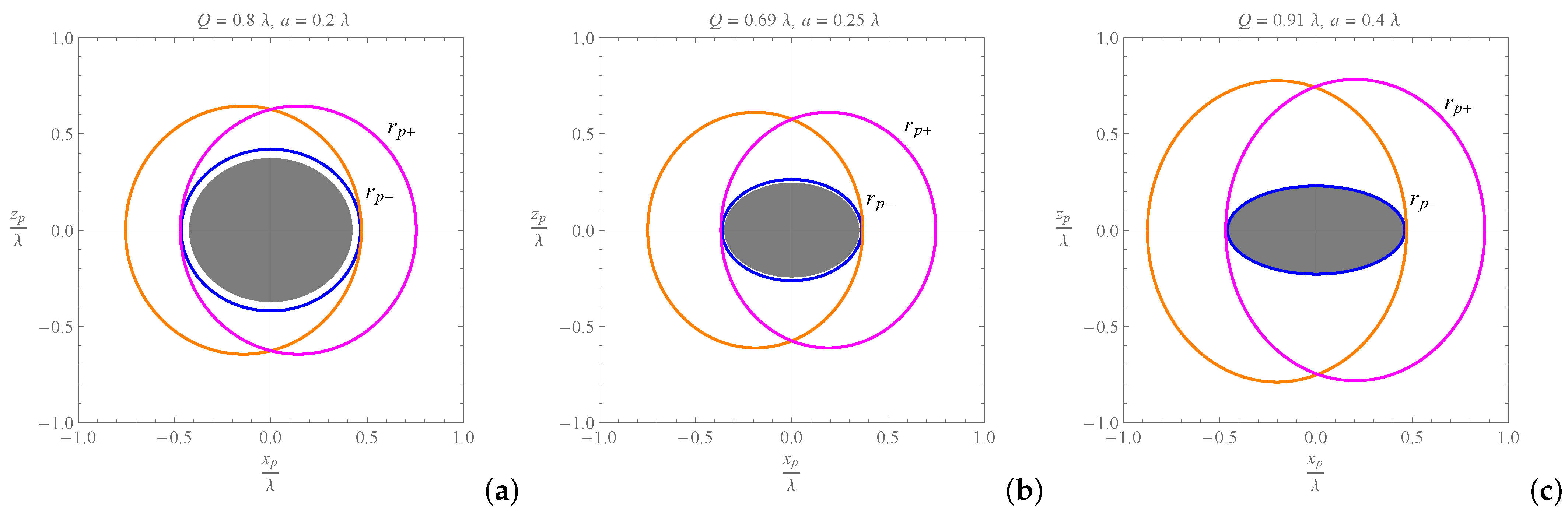
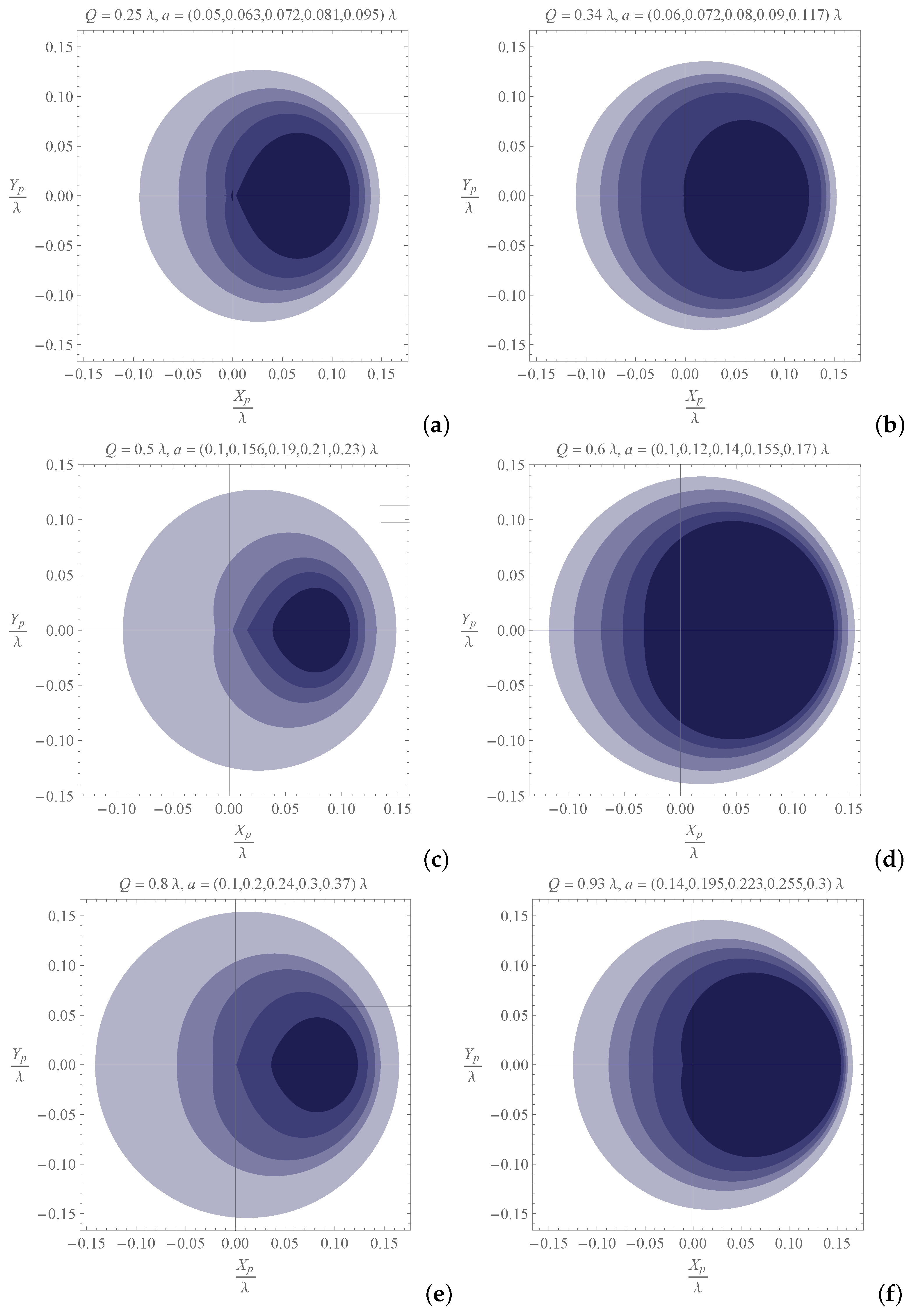
Applying the Cartesian coordinates in Equation (36), $r_{p-}$ and $r_{p+}$ and the corresponding photon regions ($r_{p-}<r<r_{p+}$) are plotted in Figure 5, together with the event horizon for some definite values of the black hole parameters. As observed from the figures, faster spinning RCWBH can produce larger photon regions.

The shape of the photon regions informs about the shape of the black hole shadow, since the shadow is confined to the photon surfaces. Those photons on unstable orbits that can reach the distant observers, can create an image of the outer regions of the event horizon. Such photons are, therefore, responsible, for example, for the image obtained from M87* [1].

To proceed with the determination of the shadow of the RCWBH, we should bear in mind that this spacetime is not asymptotically flat. We, therefore, cannot consider an observer at infinity, as is traditionally done in [71,79] and in [81]. Therefore, instead of using the celestial coordinates in the sky of an observer at infinity, we locate an observer at the coordinate position $(r_o,{\theta }_o)$, which is characterized by the orthonormal tetrad ${\mathit{e}}_{\left\{A\right\}}$, selected as

$$\begin{array}{ccc}\hfill & & {\mathit{e}}_0={\left.\frac{\left(\Sigma +a^2{\sin }^2\theta \right){\partial }_t+a{\partial }_{\varphi }}{\sqrt{\Sigma \Delta }}\right|}_{(r_o,{\theta }_o)},\hfill \end{array}$$

(61)

$$\begin{array}{ccc}& & {\mathit{e}}_1={\left.\sqrt{\frac{1}{\Sigma }}\partial \theta \right|}_{(r_o,{\theta }_o)},\hfill \end{array}$$

(62)

$$\begin{array}{ccc}& & {\mathit{e}}_2={\left.-\frac{\left({\partial }_{\varphi }+a{\sin }^2\theta {\partial }_t\right)}{\sqrt{\Sigma }\sin \theta }\right|}_{(r_o,{\theta }_o)},\hfill \end{array}$$

(63)

$$\begin{array}{ccc}& & {\mathit{e}}_3={\left.-\sqrt{\frac{\Delta }{\Sigma }}\partial r\right|}_{(r_o,{\theta }_o)},\hfill \end{array}$$

(64)

which satisfy ${e_A}^{\alpha }{e^B}_{\alpha }={\delta }_A^B$. This method, introduced in [82], makes it possible to calculate the celestial coordinates in general spacetimes with cosmological constituents (also see [83] for a review). In the above set of tetrads, the time-like vector ${\mathit{e}}_0$ is supposed to be the velocity four-vector of the selected observer. ${\mathit{e}}_3$ is set to point toward the black hole, and ${\mathit{e}}_0\pm {\mathit{e}}_3$ is the generator of the principal null congruence. In this way, a linear combination of ${\mathit{e}}_{\left\{A\right\}}$ is tangent to the light ray $\ell \left(\tau \right)=\left(t\left(\tau \right),r\left(\tau \right),\theta \left(\tau \right),\varphi \left(\tau \right)\right)$, which is sent from the black hole to the past. The tangent to this light ray can be parameterized in two ways:

$$\begin{array}{ccc}\hfill & & \frac{\mathrm{d}\ell }{\mathrm{d}\tau }=\frac{\mathrm{d}t}{\mathrm{d}\tau }{\partial }_t+\frac{\mathrm{d}r}{\mathrm{d}\tau }{\partial }_r+\frac{\mathrm{d}\theta }{\mathrm{d}\tau }{\partial }_{\theta }+\frac{\mathrm{d}\varphi }{\mathrm{d}\tau }{\partial }_{\varphi },\hfill \end{array}$$

(65)

$$\begin{array}{ccc}& & \frac{\mathrm{d}\ell }{\mathrm{d}\tau }=\mathfrak{c}\left(-{\mathit{e}}_0+\sin \vartheta \cos \psi {\mathit{e}}_1+\sin \vartheta \sin \psi {\mathit{e}}_2+\cos \vartheta {\mathit{e}}_3\right),\hfill \end{array}$$

(66)

in which, $\vartheta$ and $\psi$ are newly defined celestial coordinates in the observer’s sky and

$$\mathfrak{c}=\mathbf{g}\left(\ell ,{\mathit{e}}_0\right)=\frac{a\tilde{\mathcal{L}}-\left(\Sigma +a^2{\sin }^2\theta \right)\tilde{\mathcal{E}}}{\sqrt{\Sigma \Delta }}.$$

(67)

$\vartheta =0$ points, directly, to the black hole. Since the boundary curve of the shadow is generated by those light rays that come onto the critical (unstable) null geodesics at the radial distance $r_p$, this region, therefore, corresponds to the critical impact parameters ${\tilde{b}}_c$ and ${\tilde{\eta }}_c$, given in Equations (55) and (56). The corresponding celestial coordinates $({\psi }_p,{\vartheta }_p)$ at this distance, for the observer located at $(r_o,{\theta }_o)$, were derived as [82]

$$\begin{array}{ccc}\hfill & & \mathcal{P}(r_p,{\theta }_o)=\sin {\psi }_p=\frac{{\tilde{b}}_c\left(r_p\right)+a{\cos }^2{\theta }_o-a}{\sqrt{{\tilde{\eta }}_c\left(r_p\right)}\sin {\theta }_o},\hfill \end{array}$$

(68)

$$\begin{array}{ccc}& & \mathcal{T}(r_p,r_o)=\sin {\vartheta }_p=\frac{\sqrt{\Delta \left(r_o\right){\tilde{\eta }}_c\left(r_p\right)}}{r_o^2-a({\tilde{b}}_c\left(r_p\right)-a)}.\hfill \end{array}$$

(69)

Accordingly, the $\vartheta$ coordinate has its maximum and minimum values, respectively, for ${\psi }_p=-\pi /2$ and ${\psi }_p=\pi /2$. This helps us in obtaining the corresponding values of $r_p$ for each of the cases. Applying Equation (68), these conditions result in the equation

$$\Sigma (r_p,{\theta }_o){\Delta }^{\prime }\left(r_p\right)-4r_p\Delta \left(r_p\right)=\mp r_p\sin {\theta }_o\sqrt{16\left(a^2-\Delta \left(r_p\right)\right)\Delta \left(r_p\right)+8r_p\Delta \left(r_p\right){\Delta }^{\prime }\left(r_p\right)-r_p^2{\Delta }^{\prime }{\left(r_p\right)}^2},$$

(70)

where $\Sigma (r_p,{\theta }_o)=r_p^2+a^2{\cos }^2{\theta }_o$. This equation is of fourth order in $r_p$ and has the positive solutions

$$\begin{array}{ccc}\hfill & & r_{pmin}=\sqrt{\frac{{\overline{c}}_2}{{\overline{c}}_1}}\sin \left(\frac{1}{2}\arcsin \left(\frac{2\sqrt{{\overline{c}}_3/{\overline{c}}_1}}{{\overline{c}}_2/{\overline{c}}_1}\right)\right),\hfill \end{array}$$

(71)

$$\begin{array}{ccc}& & r_{pmax}=\sqrt{\frac{{\overline{c}}_2}{{\overline{c}}_1}}\cos \left(\frac{1}{2}\arcsin \left(\frac{2\sqrt{{\overline{c}}_3/{\overline{c}}_1}}{{\overline{c}}_2/{\overline{c}}_1}\right)\right),\hfill \end{array}$$

(72)

in which

$$\begin{array}{cc}\hfill & {\overline{c}}_1=4\left(4a^2{\cot }^2{\theta }_o\left(a^2{\cos }^2{\theta }_o+{\lambda }^2\right)-{\lambda }^2\left(4a^2+{\lambda }^2\right)+{\lambda }^4{\csc }^2{\theta }_o\right),\hfill \end{array}$$

(73a)

$$\begin{array}{cc}\hfill & {\overline{c}}_2=2{\lambda }^4{\csc }^2{\theta }_o\left(-8a^2+Q^2\cos \left(2{\theta }_o\right)+Q^2\right)+8a^2{\lambda }^2{\cot }^2{\theta }_o\left(a^2\cos \left(2{\theta }_o\right)-3a^2+{\lambda }^2+Q^2\right),\hfill \end{array}$$

(73b)

$$\begin{array}{cc}\hfill & {\overline{c}}_3=\frac{1}{2}{\lambda }^4{\csc }^2{\theta }_o\left(a^4\cos \left(4{\theta }_o\right)+\left(Q^4-12a^4\right)\cos \left(2{\theta }_o\right)+19a^4-8a^2{Q}^2+Q^4\right).\hfill \end{array}$$

(73c)

The above values are those radii where the boundary of the photon region intersects with the cone $\theta ={\theta }_o$. When $a=0$, we have $r_{pmax}=r_{pmin}=Q/\sqrt{2}$, which is the radius of the unstable photon orbits around a static CWBH, and it does not depend on $\lambda$ [53]. This unique value corresponds to the constant value of ${\vartheta }_p=\pi /2$ for $a=0$. The shadow of the static black hole is, therefore, circular.

Returning to the case of $a\ne 0$, the two-dimensional Cartesian coordinates for the chosen observer of the velocity four-vector ${\mathit{e}}_0$ are now obtained by applying the stereographic projection of the celestial sphere $({\psi }_p,{\vartheta }_p)$ onto a plane. This provides the coordinates [82]

$$\begin{array}{ccc}\hfill & & X_p=-2\tan \left(\frac{{\vartheta }_p}{2}\right)\sin {\psi }_p,\hfill \end{array}$$

(74)

$$\begin{array}{ccc}& & Y_p=-2\tan \left(\frac{{\vartheta }_p}{2}\right)\cos {\psi }_p.\hfill \end{array}$$

(75)

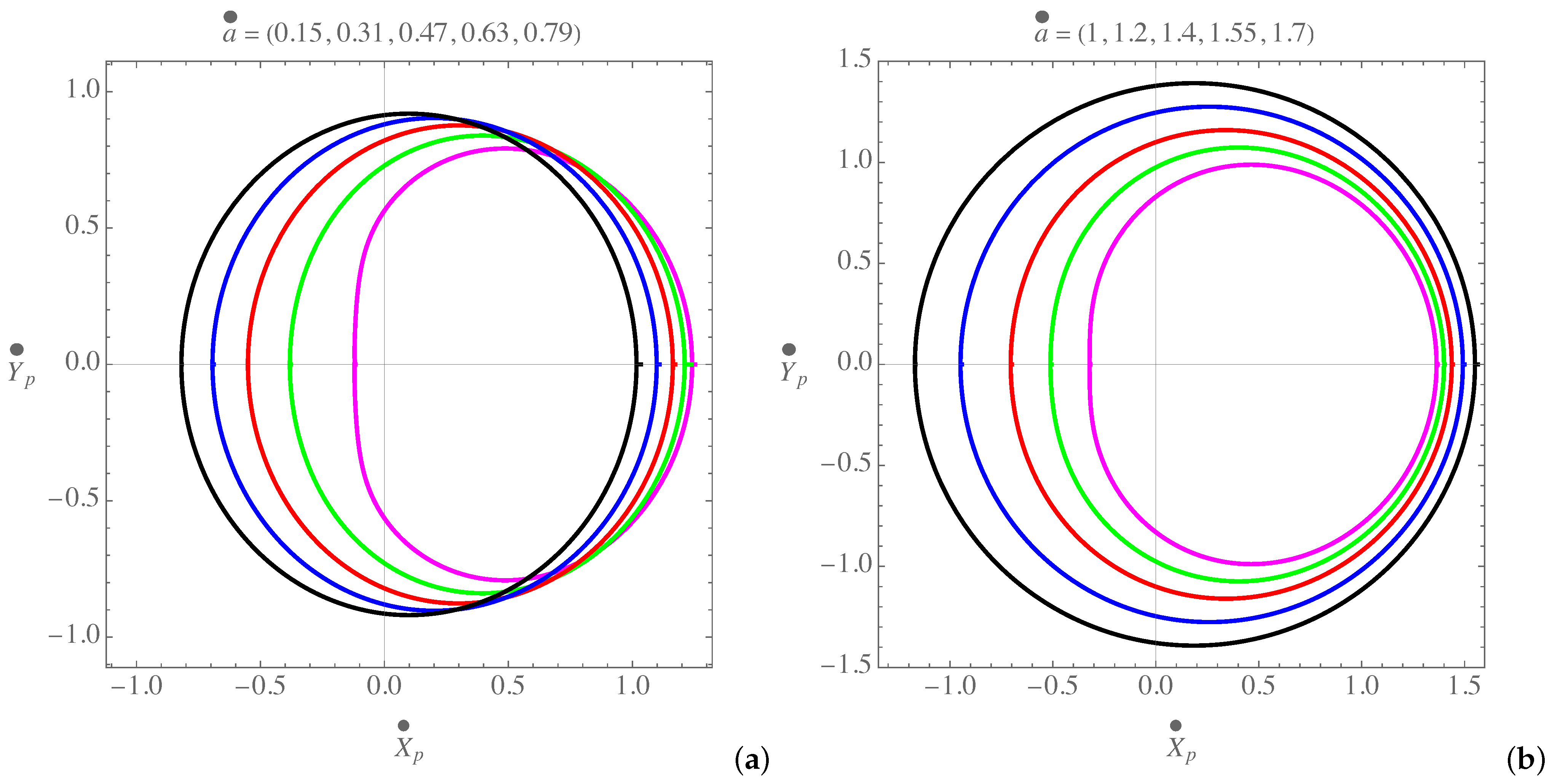
The case of ${\theta }_o=\pi /2$ corresponds to the equatorial plane of view for the observer. Taking this into account, in Figure 6, we used the above coordinates to obtain the shadow of the RCWBH for different values of electric charge and spin parameters. The curves use $r_p$ as their parameter.

In general, and for a given spin parameter, the size of the shadow increases by increasing the electric charge, and, as is inferred from the figures, by raising the black hole’s spin, the shadow shrinks and tends to the positive part of the coordinate plane. The shadow becomes oblate toward the $X_p=0$ axis from the negative sector of the coordinate plane, whereas it is sharp toward that from the positive sector. However, the amount of such deformations cannot be inferred directly from the $Q/a$ fraction and is a consequence of the spacetime’s response to the changes in the electric charge.

The size and the deformation of the shadow casts of black holes have been used to estimate their dynamical properties. In the forthcoming subsection, using a specific geometric method, we relate the angular size of a deformed shadow to the physical characteristics of the black hole. However, before proceeding with that, we make a comparison between the formation and the evolution of the shadows of the Kerr–Newman–de Sitter black hole (KNdSBH) and the RCWBH. In this way, we will be able to gain some visualizations for the differences between the general relativistic spacetimes and that of the RCWBH. The line element associated with the KNdSBH is given by [112]

$$\begin{array}{c}\mathrm{d}{s}_{\mathrm{kn}}^2=-\frac{{\Delta }_r-a^2{\Delta }_{\theta }{\sin }^2\theta }{\Sigma }\mathrm{d}{t}^2+\frac{\Sigma }{{\Delta }_r}\mathrm{d}{r}^2+\frac{\Sigma }{{\Delta }_{\theta }}\mathrm{d}{\theta }^2+\frac{2}{\Sigma }\left[{\Delta }_{r}a{\sin }^2\theta -a{\Delta }_{\theta }{\sin }^2\theta \left(\Sigma +a^2{\sin }^2\theta \right)\right]\mathrm{d}t\mathrm{d}\varphi \hfill \\ \hfill +\frac{1}{\Sigma }\left[{\left(\Sigma +a^2{\sin }^2\theta \right)}^2{\Delta }_{\theta }{\sin }^2\theta -{\Delta }_r{a}^2{\sin }^4\theta \right]\mathrm{d}{\varphi }^2,\end{array}$$

(76)

in which, the new functions

$$\begin{array}{cc}\hfill & {\Delta }_r=r^2-2M_{0}r+a^2+Q_0^2+\frac{R_0{r}^2}{12}\left(a^2+r^2\right),\hfill \end{array}$$

(77a)

$$\begin{array}{cc}\hfill & {\Delta }_{\theta }=1+\frac{R_0{a}^2{\cos }^2\theta }{12},\hfill \end{array}$$

(77b)

with $R_0\equiv 4\Lambda$, associate with a massive object of mass $M_0$ and charge $Q_0$. In [82], the shadow of the KNdSBH was calculated, using the celestial coordinates

$$\begin{array}{ccc}\hfill & & \sin {\psi }_p^{\mathrm{kn}}=\frac{1}{\sqrt{{\Delta }_{\theta }\left({\theta }_o\right)}}\sin \psi ,\hfill \end{array}$$

(78)

$$\begin{array}{ccc}& & \sin {\vartheta }_p^{\mathrm{kn}}=\sin {\vartheta }_p,\hfill \end{array}$$

(79)

which are given here in terms of those in Equations (68) and (69) and the same impact parameters in Equations (55) and (56). Defining $\stackrel{•}{\mathfrak{q}}$ as the dimension-less version of a black hole quantity $\mathfrak{q}$, re-scaled by the corresponding black hole mass parameters7, in Figure 7, we applied the Cartesian coordinates (74) and (75), to compare the shadows of the KNdSBH and the RCWBH for definite values of the black hole parameters, and for several values of the spin parameter. Having in mind the re-scaling of the coordinates, it is seen from the diagrams that the RCWBH has larger shadows than the KNdSBH, respecting their black hole masses. Additionally, the increase in the spin parameter, makes the shadow of the KNdSBH shrink outside the larger ones, whereas for the RCWBH, this happens inside of those.

The Angular Size of the Shadow

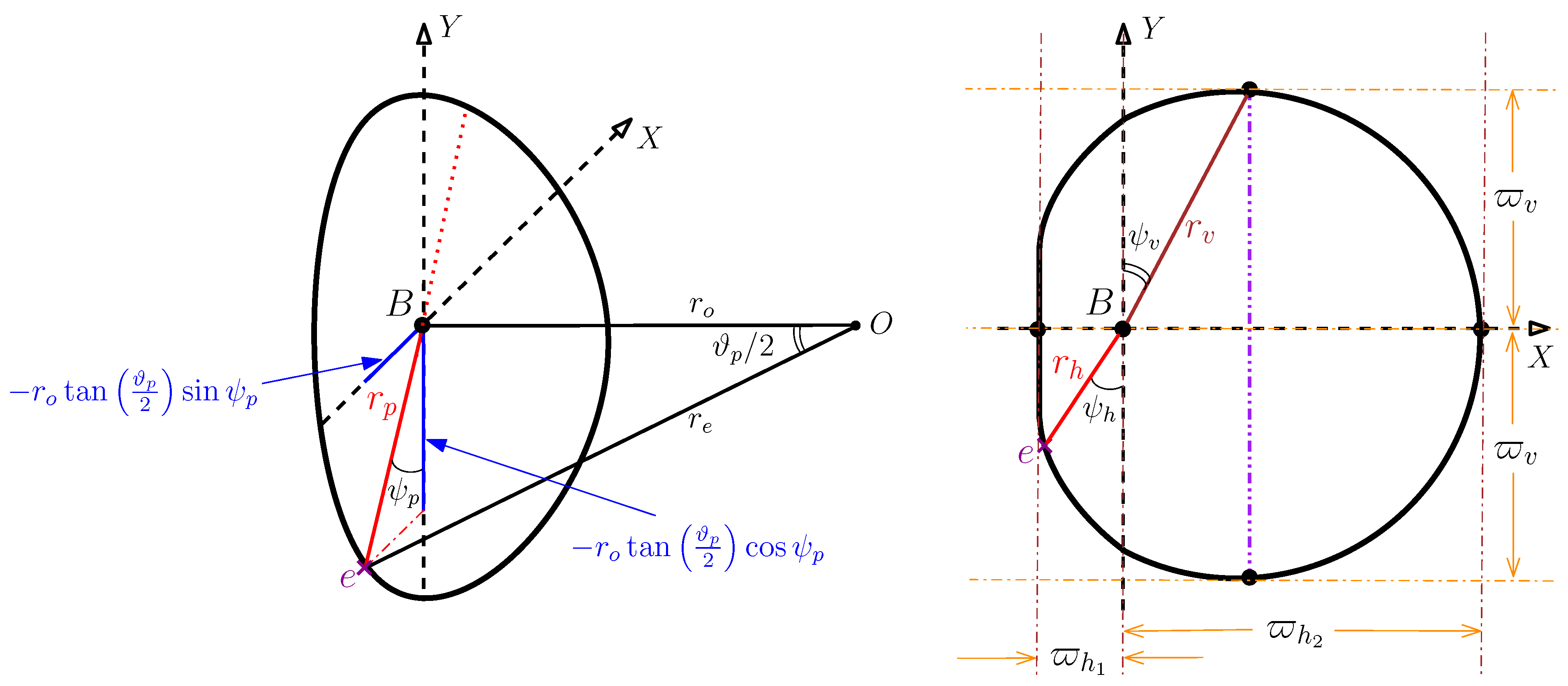
The celestial coordinates defined in Equations (68) and (69) can be used to calculate the angular diameters of the shadow. As shown in the left panel of Figure 8, these angular diameters are expressed in terms of the celestial coordinates $({\psi }_p,{\vartheta }_p)$.

Following the methods introduced in [113], we replace these angular diameters by

$$\begin{array}{ccc}\hfill & & {\delta }_h={\varpi }_{h_1}+{\varpi }_{h_2},\hfill \end{array}$$

(80)

$$\begin{array}{ccc}& & {\delta }_v=2{\varpi }_v,\hfill \end{array}$$

(81)

which are defined in terms of the three angular radii ${\varpi }_{h_1}$, ${\varpi }_{h_2}$, and ${\varpi }_v$, that obey the properties (see the right panel of Figure 8)

$$\begin{array}{ccc}\hfill & & \sin {\varpi }_{h_i}=\sin {\vartheta }_{h_i}\sin {\psi }_{h_i},(i=1,2),\hfill \end{array}$$

(82)

$$\begin{array}{ccc}& & \sin {\varpi }_v=\sin {\vartheta }_v\cos {\psi }_v,\hfill \end{array}$$

(83)

or from Equations (68) and (69),

$$\begin{array}{ccc}\hfill & & \sin {\varpi }_{h_i}=\mathcal{T}(r_{h_i},r_o)\mathcal{P}(r_{h_i},{\theta }_o),\hfill \end{array}$$

(84)

$$\begin{array}{ccc}& & \sin {\varpi }_v=\mathcal{T}(r_v,r_o)\sqrt{1-{\mathcal{P}}^2(r_v,{\theta }_o)}.\hfill \end{array}$$

(85)

Once again, we restrict ourselves to the equatorial plane by letting ${\theta }_o=\pi /2$, so that the horizontal angular diameter corresponds to ${\psi }_h=\pm \pi /2$, and we need to solve ${\mathcal{P}}^2(r_h,\pi /2)=1$ for this case. Using Equation (68) together with Equations (55) and (56), this condition provides an equation of fourth order in $r_h$, which has the positive solutions

$$\begin{array}{ccc}\hfill & & r_{h_1}=\sqrt{{\overline{C}}_1}\sin \left(\frac{1}{2}\arcsin \left(\frac{2\sqrt{{\overline{C}}_2}}{{\overline{C}}_1}\right)\right),\hfill \end{array}$$

(86)

$$\begin{array}{ccc}& & r_{h_2}=\sqrt{{\overline{C}}_1}\cos \left(\frac{1}{2}\arcsin \left(\frac{2\sqrt{{\overline{C}}_2}}{{\overline{C}}_1}\right)\right),\hfill \end{array}$$

(87)

where

$$\begin{array}{cc}\hfill & {\overline{C}}_1=\frac{Q^2-2a^2}{2\left(\frac{a^2}{{\lambda }^2}\right)+1},\hfill \end{array}$$

(88a)

$$\begin{array}{cc}\hfill & {\overline{C}}_2=\frac{2a^4-\frac{3}{2}{a}^2\left(a^2+\frac{1}{4}\right)}{\left(\frac{a^2}{{\lambda }^2}\right)+1}.\hfill \end{array}$$

(88b)

The horizontal angular radii are then calculated by evaluating the product $\mathcal{T}(r_{h_{1,2}},r_o)$$\mathcal{P}(r_{h_{1,2}},\pi /2)$, and, from there, ${\delta }_h$ can be evaluated using Equation (80). To calculate the vertical angular radius, we take into account the fact that this radius corresponds to those points on the shadow’s boundary, where the tangent to the curve $\mathcal{C}(r_v,r_o,{\theta }_o)\equiv {\sin }^2{\varpi }_v$ vanishes. Accordingly, we encounter the equation ${\partial }_{r_v}\mathcal{C}(r_v,r_o,\pi /2)=0$. Considering this condition and applying Equation (85) together with Equations (68) and (69), we obtain the unique positive value

$$r_v=r_o\sqrt{\frac{Q^2-2a^2}{2\left(a^2+r_o^2\right)}},$$

(89)

which evaluates the vertical angular radii as

$${\sin }^2{\varpi }_v=\frac{\left(Q^2-2a^2\right)\left({\lambda }^2\left(4a^2-Q^2+4r_o^2\right)-4r_o^4\right)}{8a^4{\lambda }^2+a^2\left(8r_o^2\left({\lambda }^2+r_o^2\right)-2{\lambda }^2{Q}^2\right)+4r_o^4\left({\lambda }^2-Q^2\right)}.$$

(90)

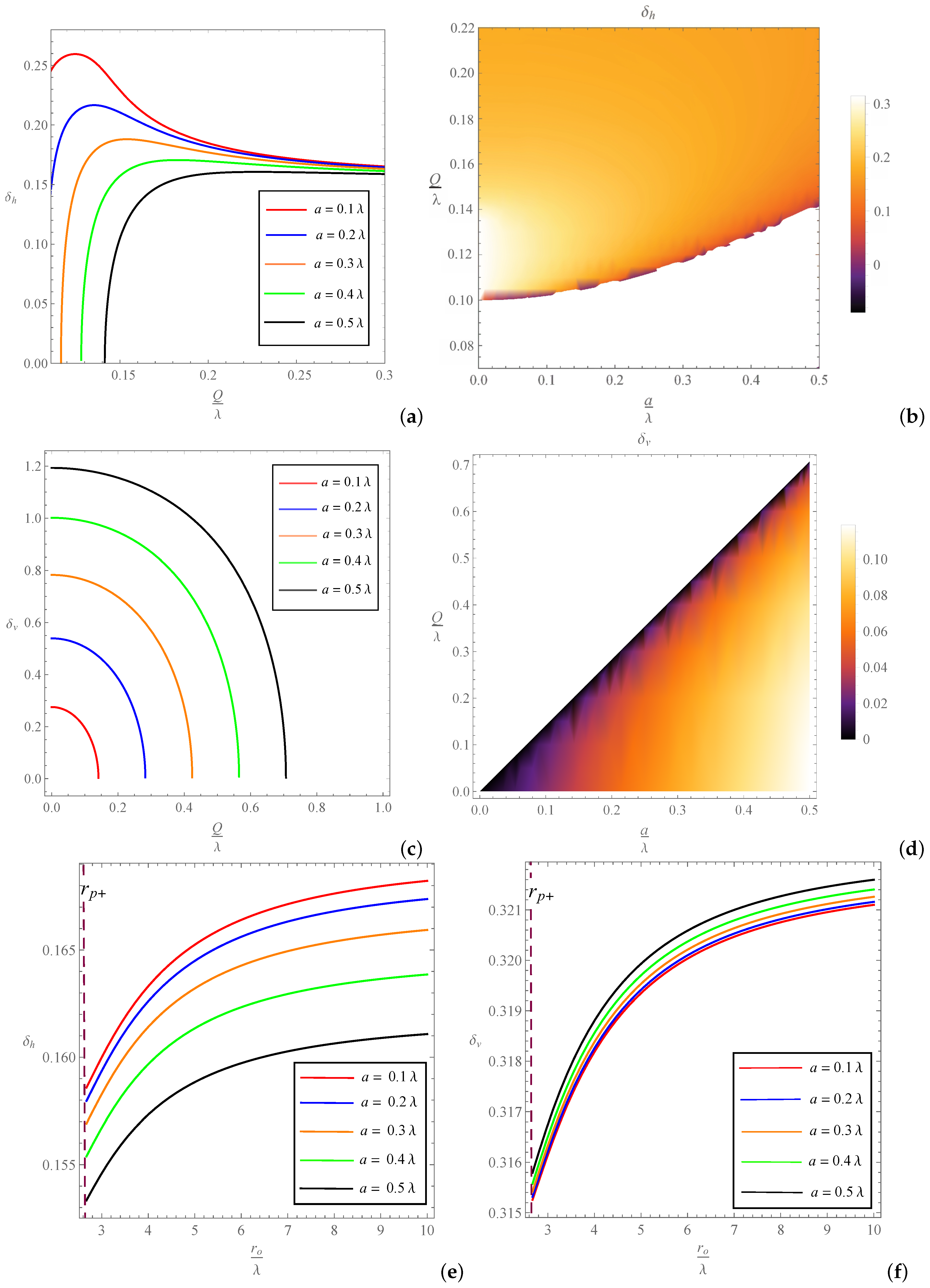
The vertical angular diameter ${\delta }_v$ can be, thus, calculated using Equation (81). In Figure 9, the behaviors of ${\delta }_h$ and ${\delta }_v$ are plotted in terms of changes in Q and a.

As observed from the diagrams, each of the horizontal diameter curves has a maximum, which is more significant for smaller a. Furthermore, the horizontal size is larger for smaller a, and all the curves tend to a same value as Q increases. On the other hand, the curves corresponding to the vertical diameter expose a smooth decrease in value with respect to increase in Q for each of the cases. An increase in the spin parameter only increases the vertical size of the shadow, and, in contrast with the previous case, the vertical size is smaller for smaller a. These can be inferred, as well, from the density plots in the right panel diagrams.

As seen in Equations (84) and (85), the other effective factor in the angular sizes of the shadow, is the observer’s distance $r_o$. As shown in the bottom panels of Figure 9, with an increase in $r_o$ outside $r_{p+}$, the shadow increases in size until its angular diameters reach a constant maximum value, within a finite distance inside the causal region. In fact, for the vertical diameter, the radial distance $r_o$ can encounter a minimum and a maximum, which can be obtained from Equation (90) as

$$r_{o\begin{array}{c}max\\ min\end{array}}^2=\frac{1}{2}\left({\lambda }^2\pm \sqrt{{\lambda }^2\left(4a^2-Q^2+{\lambda }^2\right)}\right),$$

(91)

where, $r_{omin}$ exists only for $Q>2a$, for which, $r_{p-}$ also exists. The increase in the size of the shadow by distance, is a consequence of the peculiar contribution of the cosmological term $\lambda$ for the RCWBH. This term becomes more dominant as $r_o$ increases.

It is worth comparing the above vertical diameter, with the angular diameter assigned to the shadow of M87*. In this way, we obtain an estimation for the charge component of the RCWBH if it has the same angular diameter. For M87*, located at the distance $r_{o*}\approx 5.18\times {10}^{23}\mathrm{m}$ from earth, the values associated with the lapse function components in Equation (16) are ${\tilde{m}}_{*}\approx 6.4\times {10}^9{M}_{\odot }$ and ${\tilde{r}}_{*}\approx 1.82\times {10}^{13}\mathrm{m}$ [114]. The angular diameter of the shadow was observed as ${\tilde{d}}_{*}=(42\pm 3)¯\mathrm{as}$8 [1].

To perform the comparison, we fix the cosmological component of the spacetime to the current value of the cosmological constant, by letting ${\tilde{\epsilon }}_{*}={\Lambda }_0\approx 1.11\times {10}^{-52}{\mathrm{m}}^{-2}$ [115]. Furthermore, the recent evaluation of the spin parameter of M87* is $a_{*}=0.9\pm 0.05$ [116]. Assuming these values together with the equivalence ${\tilde{d}}_{*}={\delta }_v$, and by taking into account the expression in Equation (90), we obtain $Q_{*}\approx 1.8\times {10}^{34}\mathrm{m}$. This value is approximately equivalent to $2.1\times {10}^{17}\mathrm{C}$, which is nearly the charge of ${10}^{36}$ protons9. This value corresponds to a charge density of ${\tilde{\rho }}_{Q*}\approx 8.32\times {10}^{-24}\frac{\mathrm{C}}{{\mathrm{m}}^3}$ for the black hole.

In this section, we simulated the shadow of the RCWBH and calculated its angular size, by applying the geometric method given in [113]. Furthermore, we used the shadow’s vertical angular diameter to estimate the electric charge of the RCWBH, if it is supposed to have the same characteristics of M87*. We leave the discussion at this point and summarize the results in the next section.

5. Summary and Conclusions

The application of conformal invariance in alternative theories of gravitation has had a long history among relativists and has even been considered as a tool to solve the singularity issue in general relativity [118]. In this regard, joining conformal symmetry with general relativistic black hole spacetimes, research has shown that it is possible to obtain singularity-free black holes in conformal gravity that can be confined successfully within the mass and the radiation spectrum of the Schwarzschild and Kerr black holes [119,120,121].

Static and rotating black hole spacetimes inferred from the Weyl conformal theory of gravity, on the other hand, are mostly given in terms of the Mannheim–Kazanas axially symmetric solutions to the Bach equations [24,51] and are intended to replace the astrophysical explanations, which are based on dark energy and dark matter scenarios. In this paper, however, we considered a particular solution to the Bach equations, which was specified to a spherically symmetric massive source. The rotating counterpart of this solution was obtained from the Azreg-Aïnou method. We then assessed the resultant stationary axially symmetric spacetime by calculating the variations of its horizons in terms of changes in the black hole parameters.

In fact, similar to the Plebański–Demiański class of solutions to the Einstein–Maxwell equations that are associated with a cosmological constant, the spacetime corresponding to the RCWBH contains two null hypersurfaces as the event and the cosmological horizons. This latter is the surface of infinite blue-shift, and the former coincides with the surface of infinite red-shift for the static case of a CWBH. For rotating black holes, however, the event horizon and the surface of infinite red-shift are separated. Regarding this, we calculated the position of this surface for the RCWBH and determined the static limit of the black hole’s exterior geometry on which the stationary and the static observers change their nature and commence corotation with the black hole. Accordingly, we demonstrated the variations of black hole’s ergosphere with respect to changes in the electric charge and the spin parameter.

Turning to the optical properties of the black hole, we used the first order light-like geodesic equations to calculate the light rays’ impact parameters, which enabled us to determine the unstable photon orbits and the related photon regions around the black hole. The photon region corresponds to what the distant observers would observer from the black hole. This region is therefore, the ultimate limit of black hole’s optical visibility and, in fact, confines the black hole’s shadow. To demonstrate the shadows of the RCWBH, we calculated the Cartesian celestial coordinates based on the method provided in [82].

The boundary of the shadow was shown to be both oblate and sharp toward the origin of the celestial coordinates, and, for a given charge parameter, an increase in the spin parameter shrinks the shadow, horizontally and vertically. This procedure is the reason for the shadow’s deformation. We also demonstrated this by calculating the angular sizes of an oblate shadow and applying three angular radii as proposed in [113]. For the particular case of oblate shadows, we also compared the RCWBH and the KNdSBH, which indicated the larger size of the shadow of the RCWBH, respecting the black hole masses.

The evolution of the photon region and the shadow of the RCWBH depends rigorously on the presence of an electric charge. Based on this fact, we applied the calculations corresponding to the vertical angular diameter of the shadow, to obtain an estimation for the electric charge of M87*, if it was supposed to be a RCWBH. The results indicated that this black hole will have about ${10}^{36}$ free protons to fulfill its electric charge deposit, which is about ${10}^{-21}$-times the total protons of the Sun [117]. This, in the realm of charged black holes, makes sense, because a black hole is not supposed to have active nuclear fusion. Therefore, the investigation presented here may help to understand the optical evolution of charged black hole spacetimes, which are inferred from alternative theories of gravity, as well as providing information about the impacts of the electromagnetic constituents of such spacetimes.

For future investigations, we can consider the motion of mass-less and massive test particles around the RCWBH and can investigate the relevant gravito-electromagnetic effects. These tasks are left for future studies.

References

- Akiyama, K. First M87 Event Horizon Telescope Results. I. The Shadow of the Supermassive Black Hole. Astrophys. J. 2019, 875, L1. [Google Scholar]
- Rubin, V.C.; Ford, W.K., Jr.; Thonnard, N. Rotational properties of 21 SC galaxies with a large range of luminosities and radii, from NGC 4605 /R = 4kpc/ to UGC 2885 /R = 122 kpc. Astrophys. J. 1980, 238, 471–487. [Google Scholar] [CrossRef]
- Massey, R.; Kitching, T.; Richard, J. The dark matter of gravitational lensing. Rept. Prog. Phys. 2010, 73, 086901. [Google Scholar] [CrossRef]
- Riess, A.G.; Filippenko, A.V.; Challis, P.; Clocchiatti, A.; Diercks, A.; Garnavich, P.M.; Gilliland, R.L.; Hogan, C.J.; Jha, S.; Kirshner, R.P. Observational evidence from supernovae for an accelerating universe and a cosmological constant. Astron. J. 1998, 116, 1009–1038. [Google Scholar] [CrossRef] [Green Version]
- Perlmutter, S.; Aldering, G.; Goldhaber, G.; Knop, R.A.; Nugent, P.; Castro, P.G.; Deustua, S.; Fabbro, S.; Goobar, A.; Groom, D.E. Measurements of Omega and Lambda from 42 high redshift supernovae. Astrophys. J. 1999, 517, 565–586. [Google Scholar] [CrossRef]
- Astier, P. The expansion of the universe observed with supernovae. arXiv 2012, arXiv:1211.2590. [Google Scholar] [CrossRef]
- Clifton, T.; Ferreira, P.G.; Padilla, A.; Skordis, C. Modified gravity and cosmology. Phys. Rep. 2012, 513, 1–189. [Google Scholar] [CrossRef] [Green Version]
- Weyl, H. Reine Infinitesimalgeometrie. Math. Z. 1918, 2, 384–411. [Google Scholar] [CrossRef] [Green Version]
- Riegert, R.J. Birkhoff’s Theorem in Conformal Gravity. Phys. Rev. Lett. 1984, 53, 315–318. [Google Scholar] [CrossRef]
- Mannheim, P.D. Are galactic rotation curves really flat? Astrophys. J. 1997, 479, 659–664. [Google Scholar] [CrossRef] [Green Version]
- Mannheim, P.D. Alternatives to dark matter and dark energy. Prog. Part. Nucl. Phys. 2006, 56, 340–445. [Google Scholar] [CrossRef] [Green Version]
- Diaferio, A.; Ostorero, L.; Cardone, V. Gamma-ray bursts as cosmological probes: ΛcDM vs. conformal gravity. J. Cosmol. Astropart. Phys. 2011, 2011. [Google Scholar] [CrossRef]
- Varieschi, G.U. Astrophysical Tests of Kinematical Conformal Cosmology in Fourth-Order Conformal Weyl Gravity. Galaxies 2014, 2, 577–600. [Google Scholar] [CrossRef]
- Jizba, P.; Kleinert, H.; Scardigli, F. Inflationary cosmology from quantum conformal gravity. Eur. Phys. J. C 2015, 75, 245. [Google Scholar] [CrossRef] [Green Version]
- Potapov, A.A.; Izmailov, R.N.; Nandi, K.K. Mass decomposition of SLACS lens galaxies in Weyl conformal gravity. Phys. Rev. D 2016, 93, 124070. [Google Scholar] [CrossRef] [Green Version]
- Bambi, C.; Cao, Z.; Modesto, L. Testing conformal gravity with astrophysical black holes. Phys. Rev. D 2017, 95, 064006. [Google Scholar] [CrossRef] [Green Version]
- Zhang, H.; Zhang, Y.; Li, X.Z. Dynamical spacetimes in conformal gravity. Nucl. Phys. B 2017, 921, 522–537. [Google Scholar] [CrossRef]
- Zhou, M.; Cao, Z.; Abdikamalov, A.; Ayzenberg, D.; Bambi, C.; Modesto, L.; Nampalliwar, S. Testing conformal gravity with the supermassive black hole in 1H0707-495. Phys. Rev. D 2018, 98, 024007. [Google Scholar] [CrossRef] [Green Version]
- Yang, R.; Chen, B.; Zhao, H.; Li, J.; Liu, Y. Test of conformal gravity with astrophysical observations. Phys. Lett. B 2013, 727, 43–47. [Google Scholar] [CrossRef] [Green Version]
- Caprini, C.; Hölscher, P.; Schwarz, D.J. Astrophysical gravitational waves in conformal gravity. Phys. Rev. D 2018, 98, 084002. [Google Scholar] [CrossRef] [Green Version]
- Yang, R. Gravitational waves in conformal gravity. Phys. Lett. B 2018, 784, 212–216. [Google Scholar] [CrossRef]
- Momennia, M.; Hendi, S.H. Quasinormal modes of black holes in Weyl gravity: Electromagnetic and gravitational perturbations. Eur. Phys. J. C 2020, 80, 505. [Google Scholar] [CrossRef]
- Faria, F.F. Gravitational waves in massive conformal gravity. Eur. Phys. J. C 2020, 80, 645. [Google Scholar] [CrossRef]
- Mannheim, P.D.; Kazanas, D. Exact vacuum solution to conformal Weyl gravity and galactic rotation curves. Astrophys. J. 1989, 342, 635–638. [Google Scholar] [CrossRef]
- Nesbet, R.K. Conformal Gravity: Dark Matter and Dark Energy. Entropy 2013, 15, 162. [Google Scholar] [CrossRef] [Green Version]
- Knox, L.; Kosowsky, A. Primordial nucleosynthesis in conformal Weyl gravity. arXiv 1993, arXiv:9311006. [Google Scholar]
- Edery, A.; Paranjape, M.B. Classical tests for Weyl gravity: Deflection of light and radar echo delay. Phys. Rev. D 1998, 58, 024011. [Google Scholar] [CrossRef] [Green Version]
- Klemm, D. Topological black holes in Weyl conformal gravity. Class. Quant. Grav. 1998, 15, 3195–3201. [Google Scholar] [CrossRef]
- Edery, A.; Methot, A.A.; Paranjape, M.B. Gauge choice and geodetic deflection in conformal gravity. Gen. Rel. Grav. 2001, 33, 2075–2079. [Google Scholar] [CrossRef]
- Pireaux, S. Light deflection in Weyl gravity: Critical distances for photon paths. Class. Quant. Grav. 2004, 21, 1897–1913. [Google Scholar] [CrossRef]
- Pireaux, S. Light deflection in Weyl gravity: Constraints on the linear parameter. Class. Quant. Grav. 2004, 21, 4317–4334. [Google Scholar] [CrossRef] [Green Version]
- Diaferio, A.; Ostorero, L. X-ray clusters of galaxies in conformal gravity. Mon. Not. R. Astron. Soc. 2009, 393, 215. [Google Scholar] [CrossRef] [Green Version]
- Sultana, J.; Kazanas, D. Bending of light in conformal Weyl gravity. Phys. Rev. D 2010, 81, 127502. [Google Scholar] [CrossRef]
- Mannheim, P.D. Cosmological Perturbations in Conformal Gravity. Phys. Rev. D 2012, 85, 124008. [Google Scholar] [CrossRef] [Green Version]
- Tanhayi, M.R.; Fathi, M.; Takook, M.V. Observable Quantities in Weyl Gravity. Mod. Phys. Lett. 2011, A26, 2403–2410. [Google Scholar] [CrossRef] [Green Version]
- Said, J.L.; Sultana, J.; Adami, K.Z. Exact Static Cylindrical Solution to Conformal Weyl Gravity. Phys. Rev. D 2012, 85, 104054. [Google Scholar] [CrossRef] [Green Version]
- Lu, H.; Pang, Y.; Pope, C.N.; Vazquez-Poritz, J.F. AdS and Lifshitz Black Holes in Conformal and Einstein-Weyl Gravities. Phys. Rev. D 2012, 86, 044011. [Google Scholar] [CrossRef] [Green Version]
- Villanueva, J.R.; Olivares, M. On the Null Trajectories in Conformal Weyl Gravity. J. Cosmol. Astropart. Phys. 2013, 1306, 040. [Google Scholar] [CrossRef] [Green Version]
- Mohseni, M.; Fathi, M. Focusing of world-lines in Weyl gravity. Eur. Phys. J. Plus 2016, 131, 21. [Google Scholar] [CrossRef] [Green Version]
- Horne, K. Conformal Gravity Rotation Curves with a Conformal Higgs Halo. Mon. Not. R. Astron. Soc. 2016, 458, 4122–4128. [Google Scholar] [CrossRef] [Green Version]
- Lim, Y.K.; Wang, Q.h. Exact gravitational lensing in conformal gravity and Schwarzschild–de Sitter spacetime. Phys. Rev. D 2017, 95, 024004. [Google Scholar] [CrossRef] [Green Version]
- Varieschi, G.U. A kinematical approach to conformal cosmology. Gen. Relativ. Gravit. 2010, 42, 929–974. [Google Scholar] [CrossRef] [Green Version]
- ’t Hooft, G. The Conformal Constraint in Canonical Quantum Gravity. arXiv 2010, arXiv:1011.0061. [Google Scholar]
- ’t Hooft, G. Probing the small distance structure of canonical quantum gravity using the conformal group. arXiv 2010, arXiv:1009.0669. [Google Scholar]
- ’t Hooft, G. A Class of Elementary Particle Models Without Any Adjustable Real Parameters. Found. Phys. 2011, 41, 1829. [Google Scholar] [CrossRef] [Green Version]
- Varieschi, G.U.; Burstein, Z. Conformal Gravity and the Alcubierre Warp Drive Metric. ISRN Astron. Astrophys. 2013, 2013, 482734. [Google Scholar] [CrossRef] [Green Version]
- de Vega, H.J.; Sanchez, N.G. Dark matter in galaxies: The dark matter particle mass is about 7 keV. arXiv 2013, arXiv:1304.0759. [Google Scholar]
- Hooft, G.T. Local Conformal Symmetry: The Missing Symmetry Component for Space and Time. arXiv 2014, arXiv:1410.6675. [Google Scholar] [CrossRef]
- Deliduman, C.; Kasikci, O.; Yapiskan, B. Flat Galactic Rotation Curves from Geometry in Weyl Gravity. arXiv 2015, arXiv:1511.07731. [Google Scholar] [CrossRef] [Green Version]
- Varieschi, G.U. Kerr metric, geodesic motion, and Flyby Anomaly in fourth-order Conformal Gravity. Gen. Relativ. Gravit. 2014, 46, 1741. [Google Scholar] [CrossRef] [Green Version]
- Mannheim, P.D.; Kazanas, D. Solutions to the Reissner-Nordström, Kerr, and Kerr–Newman problems in fourth-order conformal Weyl gravity. Phys. Rev. D 1991, 44, 417–423. [Google Scholar] [CrossRef] [PubMed]
- Payandeh, F.; Fathi, M. Spherical Solutions due to the Exterior Geometry of a Charged Weyl Black Hole. Int. J. Theor. Phys. 2012, 51, 2227–2236. [Google Scholar] [CrossRef] [Green Version]
- Fathi, M.; Olivares, M.; Villanueva, J.R. Classical tests on a charged Weyl black hole: Bending of light, Shapiro delay and Sagnac effect. Eur. Phys. J. C 2020, 80, 51. [Google Scholar] [CrossRef]
- Fathi, M.; Villanueva, J.R. Gravitational lensing of a charged Weyl black hole surrounded by plasma. arXiv 2020, arXiv:2009.03402. [Google Scholar]
- Fathi, M.; Kariminezhaddahka, M.; Olivares, M.; Villanueva, J.R. Motion of massive particles around a charged Weyl black hole and the geodetic precession of orbiting gyroscopes. Eur. Phys. J. C 2020, 80, 377. [Google Scholar] [CrossRef]
- Fathi, M.; Olivares, M.; Villanueva, J.R. Gravitational Rutherford scattering of electrically charged particles from a charged Weyl black hole. Eur. Phys. J. Plus 2021, 136, 420. [Google Scholar] [CrossRef]
- Mureika, J.R.; Varieschi, G.U. Black hole shadows in fourth-order conformal Weyl gravity. Can. J. Phys. 2017, 95, 1299–1306. [Google Scholar] [CrossRef] [Green Version]
- Kazanas, D.; Mannheim, P.D. General structure of the gravitational equations of motion in conformal Weyl gravity. Astrophys. J. Suppl. Ser. 1991, 76, 431–453. [Google Scholar] [CrossRef]
- Newman, E.T.; Janis, A.I. Note on the Kerr Spinning-Particle Metric. J. Math. Phys. 1965, 6, 915–917. [Google Scholar] [CrossRef]
- Shaikh, R. Black hole shadow in a general rotating spacetime obtained through Newman–Janis algorithm. Phys. Rev. D 2019, 100, 024028. [Google Scholar] [CrossRef] [Green Version]
- Johannsen, T.; Psaltis, D. Metric for rapidly spinning black holes suitable for strong-field tests of the no-hair theorem. Phys. Rev. D 2011, 83, 124015. [Google Scholar] [CrossRef] [Green Version]
- Bambi, C.; Modesto, L. Rotating regular black holes. Phys. Lett. B 2013, 721, 329–334. [Google Scholar] [CrossRef] [Green Version]
- Moffat, J.W. Black holes in modified gravity (MOG). Eur. Phys. J. C 2015, 75, 175. [Google Scholar] [CrossRef]
- Jusufi, K.; Jamil, M.; Chakrabarty, H.; Wu, Q.; Bambi, C.; Wang, A. Rotating regular black holes in conformal massive gravity. Phys. Rev. D 2020, 101, 044035. [Google Scholar] [CrossRef] [Green Version]
- Hansen, D.; Yunes, N. Applicability of the Newman–Janis algorithm to black hole solutions of modified gravity theories. Phys. Rev. D 2013, 88, 104020. [Google Scholar] [CrossRef] [Green Version]
- Azreg-Aïnou, M. Generating rotating regular black hole solutions without complexification. Phys. Rev. D 2014, 90, 064041. [Google Scholar] [CrossRef] [Green Version]
- Azreg-Aïnou, M. From static to rotating to conformal static solutions: Rotating imperfect fluid wormholes with(out) electric or magnetic field. Eur. Phys. J. C 2014, 74, 2865. [Google Scholar] [CrossRef] [Green Version]
- Poisson, E. A Relativist’s Toolkit: The Mathematics of Black-Hole Mechanics; Cambridge University Press: Cambridge, UK, 2009. [Google Scholar] [CrossRef]
- Misner, C.W.; Thorne, K.S.; Wheeler, J.A. Gravitation; Princeton University Press: Princeton, NJ, USA, 2017. [Google Scholar]
- Bardeen, J.M.; Press, W.H.; Teukolsky, S.A. Rotating Black Holes: Locally Nonrotating Frames, Energy Extraction, and Scalar Synchrotron Radiation. Astrophys. J. 1972, 178, 347–370. [Google Scholar] [CrossRef]
- Bardeen, J. Timelike and Null Geodesics in the Kerr Metric. In Les Houches Summer School of Theoretical Physics: Black Holes; CRC Press: Boca Raton, FL, USA, 1973; pp. 215–240. [Google Scholar]
- Chandrasekhar, S. The Mathematical Theory of Black Holes; Oxford Classic Texts in the Physical Sciences; Oxford University Press: Oxford, UK, 2002. [Google Scholar]
- Ryder, L. Introduction to General Relativity; Cambridge University Press: Cambridge, UK, 2009. [Google Scholar]
- Boyer, R.H.; Lindquist, R.W. Maximal Analytic Extension of the Kerr Metric. J. Math. Phys. 1967, 8, 265–281. [Google Scholar] [CrossRef]
- Penrose, R. “Golden Oldie”: Gravitational Collapse: The Role of General Relativity. Gen. Relativ. Gravit. 2002, 34, 1141–1165. [Google Scholar] [CrossRef]
- Synge, J.L. The Escape of Photons from Gravitationally Intense Stars. Mon. Not. R. Astron. Soc. 1966, 131, 463–466. [Google Scholar] [CrossRef]
- Cunningham, C.T.; Bardeen, J.M. The Optical Appearance of a Star Orbiting an Extreme Kerr Black Hole. Astrophys. J. Lett. 1972, 173, L137. [Google Scholar] [CrossRef]
- Luminet, J.P. Image of a spherical black hole with thin accretion disk. A&A 1979, 75, 228–235. [Google Scholar]
- Cunningham, C.T.; Bardeen, J.M. The Optical Appearance of a Star Orbiting an Extreme Kerr Black Hole. Astrophys. J. 1973, 183, 237–264. [Google Scholar] [CrossRef]
- Bray, I. Kerr black hole as a gravitational lens. Phys. Rev. D 1986, 34, 367–372. [Google Scholar] [CrossRef] [PubMed]
- Vázquez, S.E.; Esteban, E.P. Strong-field gravitational lensing by a Kerr black hole. Nuovo C. B Ser. 2004, 119, 489. [Google Scholar] [CrossRef]
- Grenzebach, A.; Perlick, V.; Lämmerzahl, C. Photon regions and shadows of Kerr–Newman-NUT black holes with a cosmological constant. Phys. Rev. D 2014, 89, 124004. [Google Scholar] [CrossRef] [Green Version]
- Grenzebach, A. The Shadow of Black Holes. In The Shadow of Black Holes: An Analytic Description; Springer: Cham, Switzerland, 2016; pp. 55–79. [Google Scholar] [CrossRef]
- Perlick, V.; Tsupko, O.Y.; Bisnovatyi-Kogan, G.S. Black hole shadow in an expanding universe with a cosmological constant. Phys. Rev. D 2018, 97, 104062. [Google Scholar] [CrossRef] [Green Version]
- Bisnovatyi-Kogan, G.S.; Tsupko, O.Y. Shadow of a black hole at cosmological distances. Phys. Rev. D 2018, 98, 084020. [Google Scholar] [CrossRef] [Green Version]
- de Vries, A. The apparent shape of a rotating charged black hole, closed photon orbits and the bifurcation set A 4. Class. Quantum Gravity 1999, 17, 123–144. [Google Scholar] [CrossRef]
- Shen, Z.Q.; Lo, K.Y.; Liang, M.C.; Ho, P.T.P.; Zhao, J.H. A size of ∼1 au for the radio source Sgr A* at the centre of the Milky Way. Nature 2005, 438, 62–64. [Google Scholar] [CrossRef]
- Amarilla, L.; Eiroa, E.F.; Giribet, G. Null geodesics and shadow of a rotating black hole in extended Chern-Simons modified gravity. Phys. Rev. D 2010, 81, 124045. [Google Scholar] [CrossRef] [Green Version]
- Amarilla, L.; Eiroa, E.F. Shadow of a rotating braneworld black hole. Phys. Rev. D 2012, 85, 064019. [Google Scholar] [CrossRef] [Green Version]
- Yumoto, A.; Nitta, D.; Chiba, T.; Sugiyama, N. Shadows of multi-black holes: Analytic exploration. Phys. Rev. D 2012, 86, 103001. [Google Scholar] [CrossRef] [Green Version]
- Amarilla, L.; Eiroa, E.F. Shadow of a Kaluza-Klein rotating dilaton black hole. Phys. Rev. D 2013, 87, 044057. [Google Scholar] [CrossRef] [Green Version]
- Atamurotov, F.; Abdujabbarov, A.; Ahmedov, B. Shadow of rotating non-Kerr black hole. Phys. Rev. D 2013, 88, 064004. [Google Scholar] [CrossRef]
- Abdujabbarov, A.A.; Rezzolla, L.; Ahmedov, B.J. A coordinate-independent characterization of a black hole shadow. Mon. Not. R. Astron. Soc. 2015, 454, 2423–2435. [Google Scholar] [CrossRef] [Green Version]
- Abdujabbarov, A.; Amir, M.; Ahmedov, B.; Ghosh, S.G. Shadow of rotating regular black holes. Phys. Rev. D 2016, 93, 104004. [Google Scholar] [CrossRef] [Green Version]
- Amir, M.; Singh, B.P.; Ghosh, S.G. Shadows of rotating five-dimensional charged EMCS black holes. Eur. Phys. J. C 2018, 78, 399. [Google Scholar] [CrossRef] [Green Version]
- Tsukamoto, N. Black hole shadow in an asymptotically flat, stationary, and axisymmetric spacetime: The Kerr–Newman and rotating regular black holes. Phys. Rev. D 2018, 97, 064021. [Google Scholar] [CrossRef] [Green Version]
- Cunha, P.V.P.; Herdeiro, C.A.R. Shadows and strong gravitational lensing: A brief review. Gen. Relativ. Gravit. 2018, 50, 42. [Google Scholar] [CrossRef] [Green Version]
- Mizuno, Y.; Younsi, Z.; Fromm, C.M.; Porth, O.; De Laurentis, M.; Olivares, H.; Falcke, H.; Kramer, M.; Rezzolla, L. The current ability to test theories of gravity with black hole shadows. Nat. Astron. 2018, 2, 585–590. [Google Scholar] [CrossRef]
- Mishra, A.K.; Chakraborty, S.; Sarkar, S. Understanding photon sphere and black hole shadow in dynamically evolving spacetimes. Phys. Rev. D 2019, 99, 104080. [Google Scholar] [CrossRef] [Green Version]
- Kumar, R.; Kumar, A.; Ghosh, S.G. Testing Rotating Regular Metrics as Candidates for Astrophysical Black Holes. Astrophys. J. 2020, 896, 89. [Google Scholar] [CrossRef]
- Zhang, M.; Guo, M. Can shadows reflect phase structures of black holes? Eur. Phys. J. C 2020, 80, 790. [Google Scholar] [CrossRef]
- Belhaj, A.; Chakhchi, L.; El Moumni, H.; Khalloufi, J.; Masmar, K. Thermal image and phase transitions of charged AdS black holes using shadow analysis. Int. J. Mod. Phys. A 2020, 35, 2050170. [Google Scholar] [CrossRef]
- Kramer, M.; Backer, D.; Cordes, J.; Lazio, T.; Stappers, B.; Johnston, S. Strong-field tests of gravity using pulsars and black holes. New Astron. Rev. 2004, 48, 993–1002. [Google Scholar] [CrossRef] [Green Version]
- Psaltis, D. Probes and Tests of Strong-Field Gravity with Observations in the Electromagnetic Spectrum. Living Rev. Relativ. 2008, 11, 9. [Google Scholar] [CrossRef] [Green Version]
- Harko, T.; Kovács, Z.; Lobo, F.S.N. Testing Hořava-Lifshitz gravity using thin accretion disk properties. Phys. Rev. 2009, D80, 044021. [Google Scholar] [CrossRef] [Green Version]
- Psaltis, D.; Özel, F.; Chan, C.K.; Marrone, D.P. A General relativistic null hypothesis test with event horizon telescope observations of the black hole shadow in Sgr A. Astrophys. J. 2015, 814, 115. [Google Scholar] [CrossRef] [Green Version]
- Johannsen, T.; Broderick, A.E.; Plewa, P.M.; Chatzopoulos, S.; Doeleman, S.S.; Eisenhauer, F.; Fish, V.L.; Genzel, R.; Gerhard, O.; Johnson, M.D. Testing General Relativity with the Shadow Size of Sgr A*. Phys. Rev. Lett. 2016, 116, 031101. [Google Scholar] [CrossRef] [PubMed]
- Psaltis, D. Testing general relativity with the Event Horizon Telescope. Gen. Relativ. Gravit. 2019, 51, 137. [Google Scholar] [CrossRef] [Green Version]
- Dymnikova, I.; Kraav, K. Identification of a Regular Black Hole by Its Shadow. Universe 2019, 5, 163. [Google Scholar] [CrossRef] [Green Version]
- Kumar, R.; Ghosh, S.G. Black Hole Parameter Estimation from Its Shadow. Astrophys. J. 2020, 892, 78. [Google Scholar] [CrossRef]
- Carter, B. Global Structure of the Kerr Family of Gravitational Fields. Phys. Rev. 1968, 174, 1559–1571. [Google Scholar] [CrossRef] [Green Version]
- Griffiths, J.B.; Podolský, J. Exact Space-Times in Einstein’s General Relativity; Cambridge Monographs on Mathematical Physics; Cambridge University Press: Cambridge, UK, 2009. [Google Scholar] [CrossRef]
- Grenzebach, A.; Perlick, V.; Lämmerzahl, C. Photon regions and shadows of accelerated black holes. Int. J. Mod. Phys. D 2015, 24, 1542024. [Google Scholar] [CrossRef] [Green Version]
- Akiyama, K.; Lu, R.S.; Fish, V.L.; Doeleman, S.S.; Broderick, A.E.; Dexter, J.; Hada, K.; Kino, M.; Nagai, H.; Honma, M.; et al. 230 GHz vlbi observations of M87: Event-horizon-scale structure during an enhanced very-high-energy γ-ray state in 2012. Astrophys. J. 2015, 807, 150. [Google Scholar] [CrossRef] [Green Version]
- Ade, P.A.R.; Aghanim, N.; Arnaud, M.; Ashdown, M.; Aumont, J.; Baccigalupi, C.; Banday, A.J.; Barreiro, R.B.; Bartlett, J.G.; Bartolo, N.; et al. Planck 2015 results-XIII. Cosmological parameters. A&A 2016, 594, A13. [Google Scholar] [CrossRef] [Green Version]
- Tamburini, F.; Thidé, B.; Della Valle, M. Measurement of the spin of the M87 black hole from its observed twisted light. Mon. Not. R. Astron. Soc. Lett. 2019, 492, L22–L27. [Google Scholar] [CrossRef]
- Phillips, K.J.H. Guide to the Sun; Cambridge University Press: Cambridge, UK, 1995. [Google Scholar]
- Mannheim, P.D. Making the Case for Conformal Gravity. Found. Phys. 2012, 42, 388–420. [Google Scholar] [CrossRef] [Green Version]
- Bambi, C.; Modesto, L.; Rachwał, L. Spacetime completeness of non-singular black holes in conformal gravity. J. Cosmol. Astropart. Phys. 2017, 2017, 003. [Google Scholar] [CrossRef]
- Bambi, C.; Modesto, L.; Porey, S.; Rachwał, L. Black hole evaporation in conformal gravity. J. Cosmol. Astropart. Phys. 2017, 2017, 033. [Google Scholar] [CrossRef] [Green Version]
- Zhou, M.; Abdikamalov, A.B.; Ayzenberg, D.; Bambi, C.; Modesto, L.; Nampalliwar, S.; Xu, Y. Singularity-free black holes in conformal gravity: New observational constraints. EPL (Europhys. Lett.) 2019, 125, 30002. [Google Scholar] [CrossRef] [Green Version]