Multi-Item Assessment of Physiognomic Diversity of Geocomplexes as a Comprehensive Method of Visual-Aesthetic Landscape Assessment


Polish Academy of Sciences, Institute of Geography and Spatial Organization, Twarda 51/55, 00-818 Warsaw, Poland
Geographies 2021, 1(1), 22-46; https://0-doi-org.brum.beds.ac.uk/10.3390/geographies1010003
Submission received: 29 January 2021
/
Revised: 2 March 2021
/
Accepted: 3 March 2021
/
Published: 9 March 2021
Abstract
:The paper presents the development of conceptual, theoretical, and methodological foundations of a complex and novel method for evaluating visual–aesthetic values of landscape. The novelty lies in the combination of methods for assessing the overall attractiveness of the landscape (geocomplex) and the view field (as seen from an observation point). The analysis was carried out for a highly environmentally diverse fragment of the Małopolska Upland (central Poland). The proposed method of evaluation is in two-stage procedure. At the first stage, the visual attractiveness of landscape units (geocomplexes distinguished on the basis of relief and land cover types) was calculated. The assessment took into account the diversity of landscape form and content (shape of the unit, contrast of landscape boundaries, vertical differentiation of relief and land cover, typological richness of vegetation). In the second stage, first, the view extent was determined using a specially written computer program from multiple points on a map in an assumed grid every 50 m. More than 3200 measurements were taken in a transect from an area of 8 sq. km for an area enclosing 77 sq. km. Then, in each of these 3.2 thousand delineated view reaches, the unit values of the physiognomic–aesthetic evaluation of the landscapes seen by the observer (first-stage evaluation) were counted. The developed method tries to make a conceptual–theoretical and methodological contribution to the study of physiognomy and aesthetics of landscapes, as the evaluation combines the aspects of surface and point attractiveness. Hence, the proposed method has a comprehensive character and can be a universal platform for physiognomic and landscape evaluation, also for practical purposes, e.g., nature protection, tourism development and spatial planning.
1. Introduction
The paper presents the development of conceptual, theoretical, and methodological foundations of a complex method for evaluating visual–aesthetic values of landscape [1]. The studies of physiognomy and aesthetic evaluation of landscape have been carried out for quite a long time [2] and were first inspired by the works of geomorphologists on the development of “scenery” of sculpture [3,4]. Nowadays, they are the subject of analysis of researchers of almost all fields of science, mainly natural sciences, social sciences, and humanities (in alphabetical order by anthropologists, ecologists, economists, geographers, sociologists, and urban planners), and less often technical and medical fields. This is due to the nature of the natural environment of human life, in which man realizes his own needs, including aesthetic ones, related to the desire to be in a “nice” environment. In conceptual, theoretical, and methodological terms, it is impossible to consider the issues of landscape aesthetics without referring to ontological foundations, connected with being in space [5]. Therefore, the elaboration by Ronald Hepburn [6], in which the author proves the sense and purposefulness of studying the aesthetic experience of the world outside the world of art, is considered to be a breakthrough for the development of landscape aesthetics research. Nowadays, landscape aesthetics research is stimulated by the growth of the so-called environmental awareness and the increasing importance of participatory tools in nature conservation [7]. In the last decade, landscape aesthetic and visual studies are stimulated by the development of the popular concept of ecosystem services, within which the concept of landscape services has been defined [8]. They are considered as a new way of interpreting the relationship between ecosystems and human well-being for sustainable development of landscapes [9].
In general, there are two basic ways to evaluate the physiognomic and aesthetic landscape (they are not the same concepts). The first one is essentially a sociological and psychological study and concerns the averaged visual perception by people (individuals, families, households, entrepreneurs, officials, experts, etc.) of different types (types, classes, etc.) of landscapes (views, ecosystems, geocomplexes, etc.). Surveys (questionnaires) and photographs and films or eyewitness observation in the field (e.g., by tourists) are usually used for this. There are a huge number of works on this subject, proving differences in this area due to gender, age, education, social position, cultural experience, individual hierarchy of needs, applicable canons of beauty, purpose of stay in a given place, and previous knowledge of the landscape. For example, significant differences in landscape perception between “ordinary” people (“laymen”) and the so-called experts are evidenced [10]. Comprehensive reviews of studies of aesthetic perception of landscape in various narrower subject and problem issues can be found in works [11,12], including older works in [13,14,15].
As late as the 19th century, John Ruskin believed that to experience the beauty of mountains, one must be a geologist, because it is important to understand the laws of nature that led to the formation of the Earth’s surface [16]. Among the attempts to objectify the study of landscape perception, we should discuss the concept of visible landscape (Fr. système paysage visible; [17]), in which a particularly important part is the filter of perception (filtre perceptif), which depends on the physiological, psychological, and cultural characteristics of the observer and which separates the real existing landscape (système producteur) from the uses of the visible landscape (système utilisateur).
The second group of approaches to landscape aesthetic analysis and evaluation consists of arbitrary assumptions that allow for the construction of formal indicators and criteria for evaluation. Results of landscape perception studies can be used for this purpose. There are many such studies and they mostly include formalized bonitations and evaluations of different types of spatial units. On the one hand, they may result from natural reasons (e.g., ecosystems, habitats, micro-regions, geocomplexes, and geomorphological surfaces are studied [18,19]), administrative reasons (territorial division, useful in analyses for practical purposes, e.g., in spatial planning and environmental protection [20]), and finally, they may be artificial units, e.g., geometric units of grid type [21]. On the other hand, these units can be views (view fields, view cones), where GIS techniques related to view extent determination prove to be particularly useful [20,22]. A large number of features (attributes) of landscapes and views are evaluated [23], e.g., in the study [24], twenty five indicators were used. Automatic landscape aesthetic evaluation methods are also advanced [25]. In general, indicators related to landscape diversity (biodiversity, geodiversity, etc.), including landscape metrics, are particularly popular [26,27].
In the literature, the first approach (sociological–psychological) is sometimes called direct, and the second (evaluation of views or formalized landscapes) is called indirect [28]. Other classifications assume distinguishing evaluation methods according to a key that can be called axiological [29] (ecological, aesthetic, psychophysical, psychological, and phenomenological models).
In spite of a great number of conceptual, theoretical, and methodological works, it seems that a quite important problem of aesthetic evaluation has not been satisfactorily solved. In landscape studies, from the point of view of the subject, the unit of reference is either a particular view from a particular place or places (or sets of views, including linear ones), or a real existing fragment of landscape (e.g., region, geocomplex). The viewshed assessments (view cones, et al.) are used in view studies based on methods grounded in art, architecture, and urban planning [15]. Elements such as harmony, dominants, and number and structure of plans are defined and identified [30,31]. In turn, the assessment of spatial units is dominated by assessment constructs based on the presence and contribution of features and elements of the natural environment, considered to have a positive or negative impact on landscape aesthetics. Among them, the most prominent are the methods based on the landscape diversity concept [32]. It is believed that the more varied the landscape is in terms of selected elements (relief, waters, forests, and trees), the higher its aesthetic value [14]. Interestingly, the latter assumption is also derived from natural philosophy [6].
Both the assessment of views and the assessment of landscapes (geographic regions) in the literature are quite separate conceptually and methodologically. The assessment of views is, so to speak, a “top-down” assessment that does not take into account the fact that the observer usually does not assess individual views, only a set of them. On the other hand, the evaluation of superficial spatial units, i.e., the evaluation “from below”, does not take into account the fact that the potential observer, apart from special exceptions, has no chance for a comprehensive “visual experience” for a rather prosaic reason: not every place of the analyzed spatial unit is reachable and he usually has to use available paths, trails, roads, etc.
This brings us to the formulation of the basic research problem of the present study, which is that in the aesthetic evaluation of a landscape “from below”, there is a lack of consideration of views extending from all but the points available to the observer, and that the field of view (evaluation “from above”) usually includes fragments of different types of landscapes, often evaluated in different ways. In light of this, the objectives of the study are as follows:
- Methodological aim: an attempt to construct a possibly universal and comprehensive method of landscape assessment by the observer, combining the experience of assessing both views from observation points “overhead” and “bottom view” landscapes. The proposed implementation of such a methodological objective in the light of the known and presented literature on the subject seems new and original;
- Empirical–cognitive goal: exemplification of this method on a selected example, including many views and many types of landscapes;
- The practical purpose, related to indicating the possibility of applying the proposed method in practice, e.g., planning tourist routes.
The construction of the article refers to the above objectives. First, the basic definitions, related to the topics addressed in the article, are presented (while the classical literature review, which, as mentioned, has already been presented in many works, is abandoned). Then, the methodological details of the proposed concept and the research area are described. The next subsection includes a description of the empirical results. After that, the discussion tries to compare the proposed method to other known environmental and landscape assessment tools. In assessing its usefulness, not only advantages, but also disadvantages were sought, and whether these disadvantages are surmountable is examined. The summary includes the most important conceptual–theoretical, methodological, and empirical findings, conclusions from the discussion of the results, and possibilities for further development of the proposed method.
The proposed evaluation method has been presented previously [1] and consists most generally of three steps:
- Evaluation of spatial units (overall evaluation of a “freely moving observer”),
- Determination of the view range from multiple points (viewshed, view field),
- Calculation (summation) of partial evaluations of spatial units (point 1) that are in each view (point 2).
Due to the time that has elapsed since that study, this paper uses the empirical calculations performed earlier for conceptual–theoretical and methodological deepening. Thus, the purpose of the paper is not only to present and evaluate the proposed method for assessing landscape visual attractiveness for a wider international reader, but also to recapitulate and reconstruct the assumptions in light of the experience and literature that has taken place since then (more than 20 years have passed). On the other hand, the conceptual and theoretical assumptions, the argumentation for specific methodological approaches, and the methodological details are presented in the next subsection.
2. Materials and Methods
2.1. Basic Conceptual–Theoretical Assumptions and Definitions
As mentioned in the introduction, there are a great many conceptual–theoretical approaches to the problem of landscape aesthetic evaluation, arising from the complexity of aesthetics itself in philosophical terms [33]. It seems that the most beneficial (and certainly pragmatic) would be to separate the components of aesthetic evaluation into objective and subjective (or into absolute and relative). According to this assumption, it is better to abandon the overly broad term “landscape aesthetics” and replace it with the more precise “landscape visual attractiveness” (LVA). In this paper, the latter term is understood as a function of realistically existing landscape (L) and unified norms defining a system of aesthetic values (AV):
LVA = f [L(AV)]
This concept was inspired by the mentioned study by Brossard and Wieber [17]. The aesthetic values of a landscape are its secondary feature, given by man, and therefore can be determined only on the basis of patterns recognized by him. For a specific assessment, features such as harmony, coherence, diversity, presence of anthropogenic forms, etc., may be considered. These features will depend on the aesthetic patterns adopted in a particular country, culture, or community. According to the theory of perception, they may be a component in the concept of landscape as seen at the site of the perceptual filter. Under the term of unified standards are included criteria developed on the basis of features of the real existing landscape that have the greatest influence on the evaluation.
A geocomplex was adopted as the basic unit for evaluating the visual attractiveness of a landscape. According to the definition [34], a geocomplex is a relatively closed part of nature, which forms a whole due to the processes occurring in it and the interdependence of its components. Geocomplexes were analyzed in view fields, determined for 7000 points based on view extent analysis (described further in technical details). A view field is the total area seen from a given point, including a full panorama (360°).
The diversity of geocomplexes was used as a general measure of visual attractiveness. In studies of landscape visual quality, this approach is widely used, as there is a fundamental consensus on this topic among researchers regarding the relationship of diversity to aesthetic evaluation [14,33], as well as uniqueness and naturalness [11,13,32].
Thus, the physiognomy of an environment is defined by its physiognomic diversity. In this sense, physiognomic landscape and natural landscape overlap. Each view is characterized by spatial relationships and the way this space (i.e., content) is filled, changing over time. Therefore, the following aspects of physiognomic diversity are proposed:
- Diversity of form, where the shape and size of the unit (geocomplex) and the contrast with the surroundings play a fundamental role;
- Diversity of content (internal diversity), defined by the richness of the building elements, their colors, and their arrangement, and the vertical extension of the landscape.
The criteria were then identified in detail. At the same time, a very rich and diverse set of them can be found in the literature for evaluating landscapes, discussed in the introduction. According to this, the physiognomic diversity of a landscape defines various features characterizing its physiognomy (external appearance). All attributes of this physiognomy should be analyzed: shapes, colors, sizes, similarities and differences in appearance (i.e., contrast), and mutual position (i.e., arrangement or harmony). Also important is the internal structure, understood as the richness and typological diversity of the elements and their arrangement (filling).
The following formula for assessing the physiognomic diversity of designated geocomplexes was proposed:
- LVA = DF + DB − H, where:
- DF—form diversity
- DB—content (body mater) diversity
- H—negative impact of human activity
of which:
- DF = Da + Dc, where:
- Da—area diversity
- Dc—contrast diversity between landscapes
and
- DB = Dr + Dv + Dd, where:
- Dr—vertical diversity of the relief
- Dv—vertical variation of vegetation (land cover)
- Dd—typological richness of vegetation
The diversity of form is the diversity of the unit’s contour. It is superior to the diversity of content. It is determined by the boundaries of the geocomplex. Often the shape and size of a unit, especially for the most variable elements (vegetation, soils), determines the internal structure, that is, the nature of what and how it fills its interior.
It is understandable that the analysis in this case depends on the scale of the subdivision and thus on the rank of the separations. The problem, on the other hand, is to establish a measure; or, in other words, an assumption as to which feature of the landscape is assessed and how it affects its physiognomy. It is understandable that this measure will depend on the purpose of the study. In order to show the compactness of the landscape, indicators of circularity, fragmentation, etc., are useful. It should be noted here that two units with different area and circular shape will have the same circularity index (always equal to 1). Therefore, it seems that the feature that characterizes well the physiognomic aspect of the surface and contour of a geocomplex is the length of its boundaries per unit area and the description of the shape of the analyzed unit.
The contrast of boundaries is more pronounced the more boundaries of lesser rank run through a site. For example, the boundary between a field on a plain and a meadow in a depression is more contrastive than the same land uses within a single relief unit. At the same time, some types, especially land cover, are “inherently” contrasting. For example, a field and meadow boundary on a plain is much less legible than a forest and field boundary.
The diversity of content, or internal diversity, determines the internal structure of the physiognomic landscape. Since this landscape (geocomplex) is distinguished on the basis of two basic elements, land cover and landform, diversity of content characterizes the diversity of these elements. It was assumed that this diversity is formed by vertical extension, richness, color, and arrangement of lower-order elements.
Vertical stretch is particularly important in the case of relief. Vertical characteristics, for comparability, are conveniently described by either relative heights or density of horizons or other multiple landscape metrics of geodiversity [35,36,37]. In the case of land cover, vegetation height can be calculated.
Internal richness is understood as the number of all elements and also the number of types. This is particularly important in the case of vegetation analysis, where the number of species or genera (depending on the scale of the study) should be considered first of all.
The diversity of the physiognomy of the geocomplex is also defined by its colors. Although the differences in colors are perfectly noticeable, this is the most difficult element to specify and evaluate and therefore was not considered in this study.
Elements that build the landscape are located in relation to each other in a characteristic, peculiar way, that is, they form a certain arrangement (texture), described as harmonious or disharmonious, open, encrusted, fenced, labyrinthine, etc. [38]. Thus, in the physiognomy of the separated landscape, it is the arrangement of clumps of trees (single, island, linear along roads), the distribution of fields (levee, block, strip), the number of plans, the composition of patches, compositional axes, the arrangement of landscape interiors, walls, gates, etc. In addition, landscapes of lower rank form characteristic arrangements, e.g., island arrangement of pine landscapes on dunes and riparian landscapes between these hills in depressions [39,40]. Moreover, the arrangement of the landscapes themselves may also be characteristic (banded in a large valley along its slopes, concentric in depressions, etc.). Measures of commonness, uniqueness, or uniformity may apply here [26].
In principle, all elements of internal landscape variation are subject to variation over time. Of course, the rate of this varies greatly. In the case of vegetation in a temperate climate such as Poland, it is an annual and daily rhythm. For example, many geophytes bloom at specific times of day or depending on the weather. It is also important to remember that color saturation is dependent on light intensity, which is simply a function of light and weather conditions. For this study, the assessment includes daytime weather conditions with moderate to full sunlight and when vegetation is fully covered (late spring, summer, and fall).
The third element of the assessment is the most subjective and involves determining the adverse impact of human activity on the visual attractiveness of the landscape. In those units, where this influence is unfavorable, the index should certainly be decreased. Such elements as, e.g., presence of transmission or telephone lines, roads with hardened surface, presence of landfills, garbage dumps, general littering, trampling, etc., should be considered unfavorable. Such solutions have been common in other works for a long time [13], especially in areas heavily transformed by humans [41].
where:
- LVA—landscape visual attractiveness,
- Da—differentiation of area = L/A, where L—circumference of the unit, A—area,
- Dc—differentiation of contrast of landscape boundaries,
- Dr—vertical differentiation of relief, expressed by the density of contour line,
- Dy—vertical differentiation of land cover, expressed by the height of the vegetation layer,
- Dd—typological richness of vegetation, expressed by the number of species (genera or other taxon, depending on the scale),
- H—indicator of unfavorable impact of human activity.
2.2. Study Area
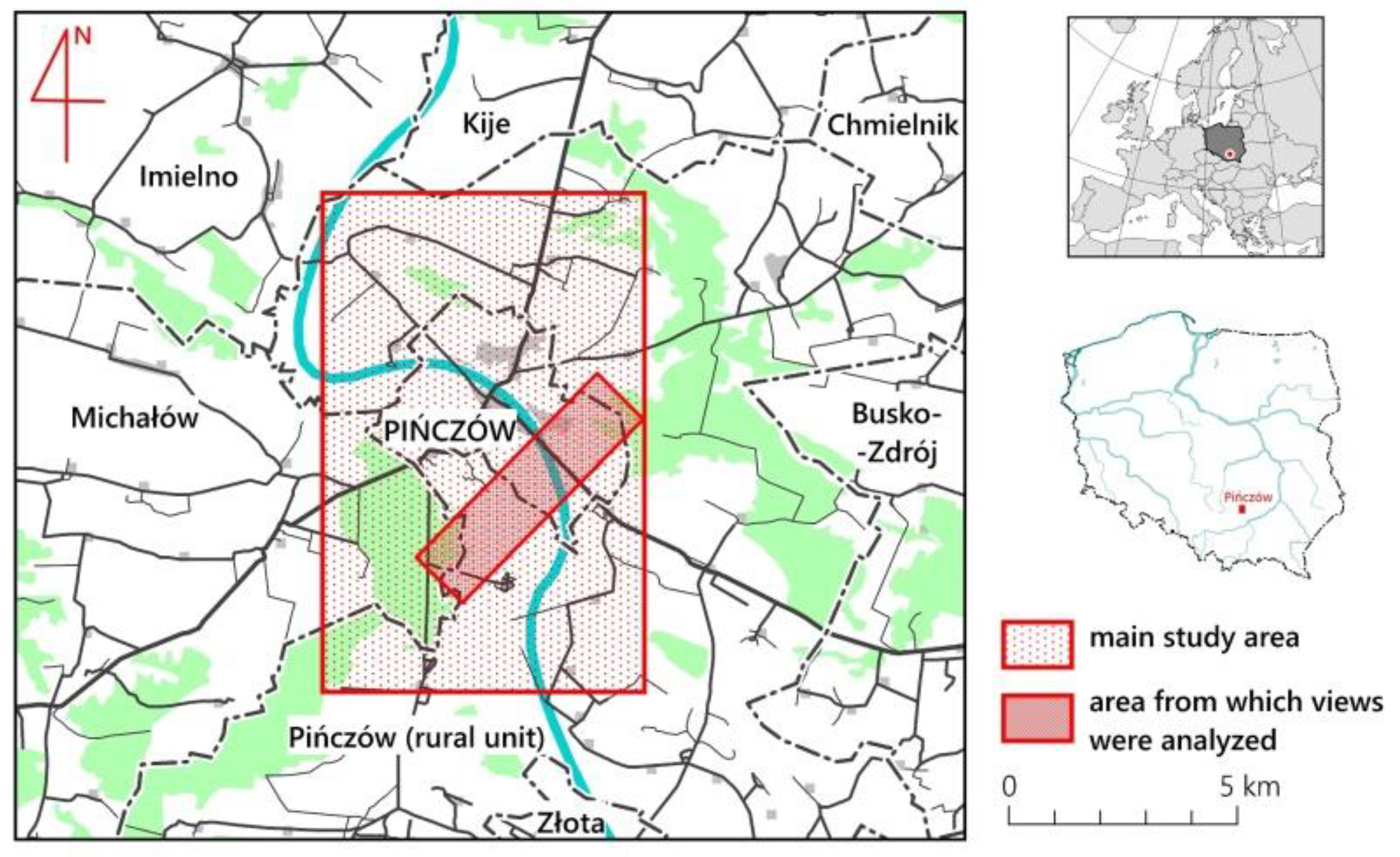
The study area selected for detailed analysis with an area of 77 sq. km is located in southern Poland in Świętokrzyskie Voivodship within the municipalities of Busko-Zdrój, Chmielnik, Imielno, Kije, Pińczów, and Złota (Figure 1). It is a rectangle of 711 km in size, bounded by a kilometer grid (1965 coordinate system: 460 to the north, 601 to the east, 449 to the south, and 594 to the west). Physico-geographically (according to delimitation [42]), it is located within the Nida Basin macro-region in mesoregions Nida River Valley (59.7%), Wodzisław Hummock (17.7%), Pińczów Hummock (15.3%), and Połaniec Basin (7.3%). The lowest place is in the Nida valley, on the southern boundary of the study area (181 m a.s.l.); the highest is the culmination of the north-western part of the Pińczów Hummock (291 m a.s.l.). The relative height is therefore 110 m. The town of Pińczów (about 11,000 inhabitants) is located in the central part of the study area, covering about 4 sq. km. The adopted scale of the study is 1:25,000.
The choice of the study area was based on several considerations. Firstly, the area is well recognized in terms of physico-geographical features. Since the 1960s, the Pińczów area has been a “testing ground” for various types of geographical research [43,44,45]. Obviously, it is not the only region in Poland so well recognized, but the fact that the natural environment here is very diverse was of key importance. The second reason was the willingness to perform analyses in an area rich in various geomorphological forms (such as valleys and slopes in particular), as well as in flora and various forms of land cover. This was also the case, because from a typological point of view, the study area consists of valleys and depressions as well as gypsum, limestone, and loess uplands [43,44], providing a great richness of vegetation and land cover.
The area is cut by the meandering, flat valley of the Nida river, a left tributary of the Vistula. In its northern part, the gypsum–limestone anticline Pińczów Hummock is well visible, rising to over 80 m above the valley. This anticline extends eastward, in the north-eastern part of the study area, becoming the Połaniec Basin. Fragments of this part of the Połaniec Basin are also called Jędrzejów Plateau. At the southern foot of the Pińczów Hummock, the historic town of Pińczów is located. On the southwestern edges of the study area rises a small fragment of Wodzisław Hummock, while on the southeastern edges is the Solec Basin. Larger concentrations of forest are found in the northeastern and southwestern portions. The area is dominated by fragmented agriculture. Cereal and root crops are characteristic, and meadow land dominates in the Nida River Valley.
In the study area, a sub-area related to the view range analysis with an area of 8 sq. km was also delimited. It was delimited in such a way as to provide a wide divergence of the view range and visibility of different landscapes. Hence, it is located along the eastern slope of Pińczów Hummock.
Overall, the study area represents an arbitrarily and geometrically delineated area fragment. As mentioned, the intention was to define it in such a way as to include different landscape units in a limited section. The proposed study area seems to meet well the analytical needs of testing the proposed landscape assessment method in the actual field. The author’s personal attitude to the area, related to his acquaintance with the Pińczów region, also played a role in the selection.
2.3. Determination of Geocomplexes
Since the visible landscape, according to Gestalt theory [33], is perceived as a whole, it is not purposeful to study the variation of its individual components (components). The study of landscape physiognomy must therefore be based on the study of the whole landscape. The most important role in the perception process is played by spatial relations (most often the size and shape of forms) [5,38], so the reference for the diversity object should be the surface. In environmental physiognomy, the following two elements are the most important: landform and land cover [13]. Therefore, the separation of geocomplexes for physiognomic analysis should be based primarily on these two elements.
In the first case, an unpublished map of landforms made during student field practice in geography in the 1990s under the direction of Dr. Bogumił Wicik (Faculty of Geography and Regional Studies, University of Warsaw) was used. The classification of relief was based on a morphological–genetic approach. The map was made at a scale of 1:25,000 and for the purposes of this study was generalized to the scale of 1:75,000, while in the case of land cover, the map of real vegetation of the Pińczów area [44] at a scale of 1:75,000 was used.
Nine types of relief were distinguished. While distinguishing relief types, attention was paid to their physiognomic features. In the Nida valley, the proper valley bottom, overflow terrace, and and plains of old glacial terraces, originating from the Middle Poland (Riss) and North Poland (Weichselian) glaciations, were distinguished. Fragments of these terraces are also found on Pińczów Hummock. Moreover, fields of wind-blown sands, glacial outcrops, flattened areas, weakly and strongly sloping slopes, as well as dry valleys and indentations are distinguished. In terms of area, the valley floor dominates, accounting for a total of 13.9%, and in terms of the number of individual contours, dry valleys and indentations dominate (158; more than a quarter of the number of all units).
Land cover types (10 types) were also separated based on physiognomic variation. Wet meadows and pastures occur mainly in the Nida valley, and grasslands and dry meadows in Pińczów Hummock, which is habitat-specific. In the group of shrubs, individual phytosociological classes were not distinguished due to their too high diversity (several types would have to be distinguished). Additionally, pine forests were not divided, because the differences between them are expressed only in the undergrowth, and physiognomically the forests do not differ. Buildings and orchards were combined into one unit, because they constitute a specific complex in the Pińczów region. These units were not assessed. Similarly, waters (Nida, oxbow lakes) and pits were not assessed. In total, the unassessed areas cover 8.5 sq. km, which is 11.0% of the total study area.
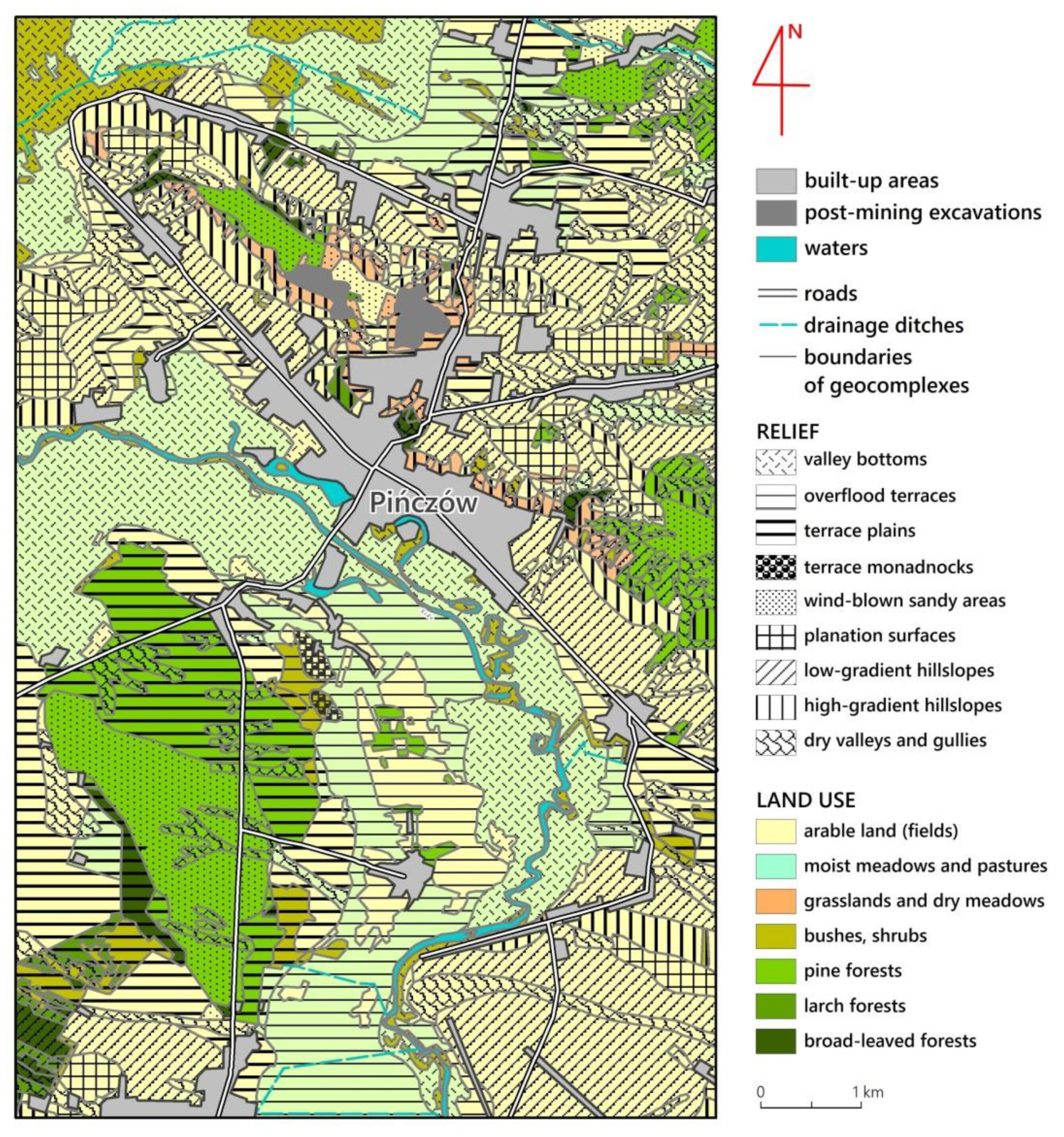
The delineation of geocomplexes was done by overlaying both maps. This resulted in the map presented in Figure 2. A total of 497 units representing 56 relief and cover types were delineated (Table 1). The areas of the patches are diverse. The largest are represented by moist meadows in the flat valley bottom (maximum about 4.7 and 3.2 sq. km) and on terraces. The smallest, reach 0.001 sq. km (1000 sq. m). Most units are small, not exceeding 5 ha (67%), as a result of fragmented agriculture.
Some geocomplexes are not entirely contained within the study area. These are the units through which the boundary of the study area runs (rectangle 711 km). It was assumed that the parts contained in the study area are representative for the whole geocomplex, and individual indicators were calculated for such areas. Part of the boundary of such units is the boundary of the study area.
2.4. Detailed Criteria for Assessing the Visual Attractiveness of Geocomplexes
The next step was to specify quantitative and qualitative criteria for assessing the visual attractiveness of the landscape. The proposed measures are the author’s subjective concept (Table 2 et seq.), previously presented in Polish [1].
The boundary shape and length index (Df) within each unit was calculated by the ratio of perimeter to occupied area. The smaller the value of the ratio, the denser the network of boundaries for a given area. The contrast index (Dc) was determined arbitrarily for different neighborhoods found within the study area (Table 3). Because vegetation plays the most important role for border contrast in the Pińczów area, only the most important cover elements were included in the differentiation. Vertical extent, calculated for relief, is the ratio of the length of the contour lines to the area (Table 4), and for land cover, the height of the vegetation layer was calculated (Table 5). Species richness was expressed by the number of species (genera) of vegetation found in the unit (Table 5). Content diversity is the arithmetic mean of these three characteristics.
The most contrasting boundaries were found to be those between water and scrub, and between forests and fields or meadows and is 5 (Table 3). Lower contrast was found for borders between fields and meadows with water (4) and between scrub and fields (3). Boundary contrast index values equal to 2 were assigned to the remaining types of cover boundaries found in the study area. It was considered that the relief boundaries in the study area are not contrastive, as they pass smoothly and were assigned the lowest index value of 1. The highest value (5) is achieved when the assessed unit is an “island” in another contrastive unit. It is, for example, a forest among fields or a shrubby island in the Nida river.
Almost all geocomplexes border on several (dozen) other, different geocomplexes. It was assumed to be the arithmetic mean of all partial contrast indices of geocomplex boundaries (average weighted by the length of individual boundaries).
As far as vertical differentiation is concerned, in the vicinity of the Pińczów terrain is unusual: next to the almost flat Nida valley, the Pińczów Hummock is located with almost “mountainous” height differences. Values from 1 to 5 were assigned according to the degree of differentiation of individual land forms (Table 4). It was taken into account that the dry valleys and indentations in Pińczów Hummock have a greater differentiation than within the terraced edges in the Nida valley (this is due to much greater differences in relative heights).
For the variation in the vertical land cover and for the vegetation richness, the index values shown in the Table 5 were adopted. It can be seen here that the same type of land cover can have different indices: grasslands and dry meadows are low, but have very high typological richness. On the other hand, monoculture larch forests fill the space, but at the same time have the lowest typological richness. The most similar index values characterize the arable fields: the index of vertical differentiation due to the low height of crops was set at 1.5, while the typological differentiation was set at 1. The other cover types are characterized by a greater difference in the index values.
Since all components are assigned equal importance for visual attractiveness, their values were transformed so that the lowest and the highest value in the each group was equal. The values from 1 to 5 were set for the absolute data (shape diversity) and vegetation. Therefore, the value of the surface diversity index should also be reduced to these values, using the formula based on Thales’ theorem:
where:
- —new value
- —old value
- —maximum new value
- —minimum new value
- —maximum old value
- —minimum new value
After replacing the known minimum and maximum values, we obtain for the area diversity index:
The last element of the assessment are the factors that have a negative impact on the visual attractiveness of the landscape. As it is impossible to determine which of the natural features have such an effect, the influence of human activity remains. In the Pińczów area, the negative influence is certainly exerted by such elements of infrastructure as transmission lines, hard surfaced roads, and various types of landfills and dumps. The influence of the vicinity of human settlements, especially urban ones, is indirect: the bordering areas are usually condemned to littering, trampling, etc. It was assumed as in Table 6.
At the same time, some anthropogenic elements in the Pińczów area were found to have no significant impact on the visual attractiveness of the landscape. These include field roads, paths, and ditches. The index of unfavorable influence of human activity was calculated by summing up the components characterizing a given unit from the table, and the obtained values were reduced to the minimum value of 1 and maximum value of 5 (as in the case of the shape diversity index).
In the vicinity of Pińczów, it is difficult to find elements of human activity that would increase the visual attractiveness of the landscape. Undoubtedly, the aesthetics of the place is enhanced by historic architecture, but the built-up areas (including Pińczów) were not assessed.
2.5. Viewshed
Determining the range of a view from a point on a map requires relatively simple calculations between the point of observation and the surroundings, but is very tedious when operating without computer assistance. Such analyses were performed even before World War II for military purposes based on detailed topographic maps. On the other hand, computer measurement of view range was probably proposed as the first in the world by E.L Amidon and G.H. Elsner [46], preparing the Viewit algorithm in the Fortran program. Nowadays, many computer programs have such functions. Unfortunately, none of them has the possibility of more complicated calculations concerning the features of individual views, of the kind of the conducted evaluation of geocomplexes. Hence, it was necessary to prepare special software.
The calculation algorithm was developed in Visual Basic program. The detailed methodology of calculations and description of results is presented in [47]. The program code, 196 lines long, was written by IT specialists Andrzej Jarosz and Tomasz Pecko. Due to IT limitations related to computing time, it was decided that the view coverage and its analysis should be carried out on an area of 8 km2 with points spaced every 50 m. After exclusion of the area occupied by forests, it was 3241 points. The calculations took into account that the height of the observer is 1.7 m.
2.6. Assessment of Attractiveness of Views
The assessment of the visual attractiveness of the landscape based on the diversity of the view field is an extension of the method described previously starting from the assessment of the physiognomic diversity of the landscape [1]. As mentioned before, the main disadvantage of the method of assessing visual attractiveness of a landscape is that it does not take into account the views from particular viewpoints. In the field of view, there are usually fragments of different types of landscapes, often evaluated in different ways.
Since it is difficult to determine the qualitative influence of individual parts of the landscape on the overall view assessment, it was assumed that individual fragments of landscape types in the field of view are proportional to their size (area occupied) and to the value of the individual indicator of landscape visual attractiveness, which characterizes particular geocomplexes. The influence of the distance of the view from the observation point, on which the perception of view diversity depends, should also be taken into account. It seems that this influence decreases proportionally to the increase of the distance:
- LAV = V × LVA, where:
- LAV—visual attractiveness of the viewshed (view field),
- LVA—visual attractiveness of the landscape, with the closest landscape having the highest importance and the one lying farthest away having the lowest,
- V—total area of the viewshed (view field).
It is fundamental for further considerations to determine the effect of distance on the perception of visual attractiveness of the landscape. Probably it has a logarithmic character. However, it should be noted that as the distance increases, the view area increases. At the same time, the sum of different aesthetic values (visual attractiveness) reaching the observer from particular landscapes also increases. The greater the sum of the values reaching the observer, therefore, the greater the extent of the view or (and) the greater the visual attractiveness indices of the landscape. Therefore, the visual attractiveness of the view field was assumed to be the sum of the products of the sizes of the seen areas of the landscapes and the visual attractiveness indices that characterize them:
- , where:
- —visual attractiveness of individual landscapes (geocomplexes),
- —areas of individual landscapes (geocomplexes).
The visual attractiveness score of a view field is therefore a weighted score. To calculate the visual attractiveness of a view field, one must determine the extent of the view and determine what geocomplexes and what parts of them are within the view. Next, you need to multiply the indicators of visual attractiveness of geocomplexes by the area they occupy in the designated view. Finally, the obtained partial ratings must be summed.
The largest values of the index calculated in this way indicate the greatest extent of the view, in which the natural environment is maximally diverse and least transformed by man. Medium values may refer to high view range and low natural diversity or low view range but with high diversity, as well as medium diversity and medium view range. The smallest values characterize views with low range and little diversity.
Since it is difficult to determine the qualitative influence of individual parts of the viewed landscape on the overall view assessment, it was assumed that individual fragments of landscape types in the field of view contribute proportionally to their size (area occupied) and to the value of the individual index of landscape visual attractiveness that characterizes particular geocomplexes.
Assessment of view attractiveness can be carried out in two main aspects:
- (a)
- as an assessment of the attractiveness of individual views or parts of views;
- (b)
- as an assessment of attractiveness of views of the same landscape, but viewed from different locations.
In case of the first approach, the result of the analysis will be an overall assessment of view attractiveness. The selection of points from which the attractiveness of views will be assessed can be done by creating a geometric grid, or by choosing points in characteristic places (ridge lines, hill tops, etc.). Using the second approach, we will get an answer to the question of where the most attractive view of a given geocomplex comes from. It is understandable that the aesthetic perception of the same landscape is different when viewed “overhead” (top-down) and “bottom”. In further considerations, the first approach is adopted. It is methodically simpler and technically less complicated to implement.
2.7. Tool and Technical Explanations
As mentioned, the computation of the view extent and the computation of the features of the fragments of landscape types located in the individual views were performed based on a specially written code in Visual Basic program. The code was written by Andrzej Jarosz and Tomasz Pecko in 1996, according to the instructions of the author of this paper (Supplementary Material). The use of existing software solutions for view extent analysis was not justified, because none of the software packages have extensions that allow analysis of visibility elements related to their synthetic differentiation. Other analyses, calculations, and visualizations were performed in MapInfo Professional software.
3. Results
3.1. Assessing the Visual Attractiveness of Geocomplexes
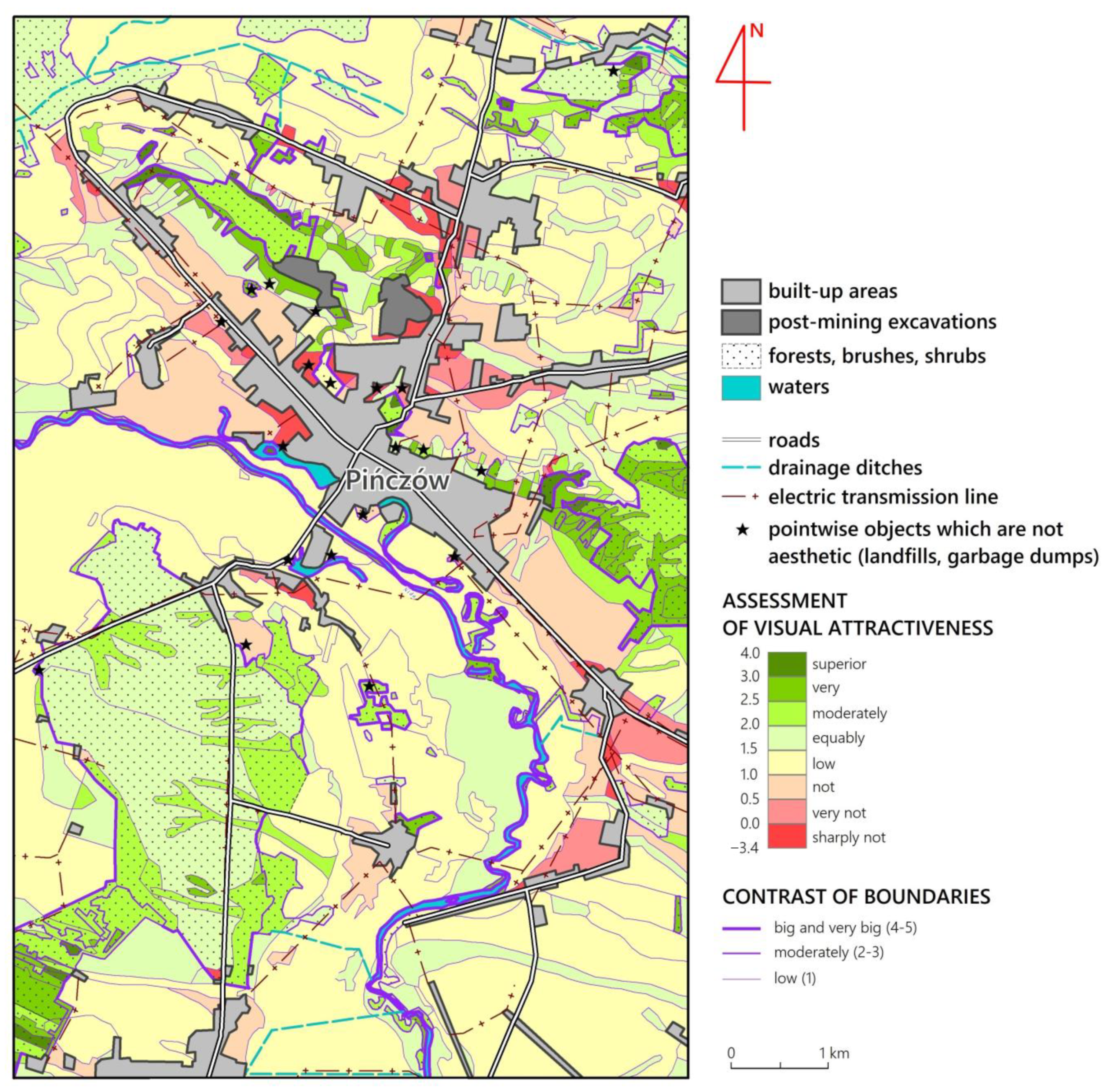
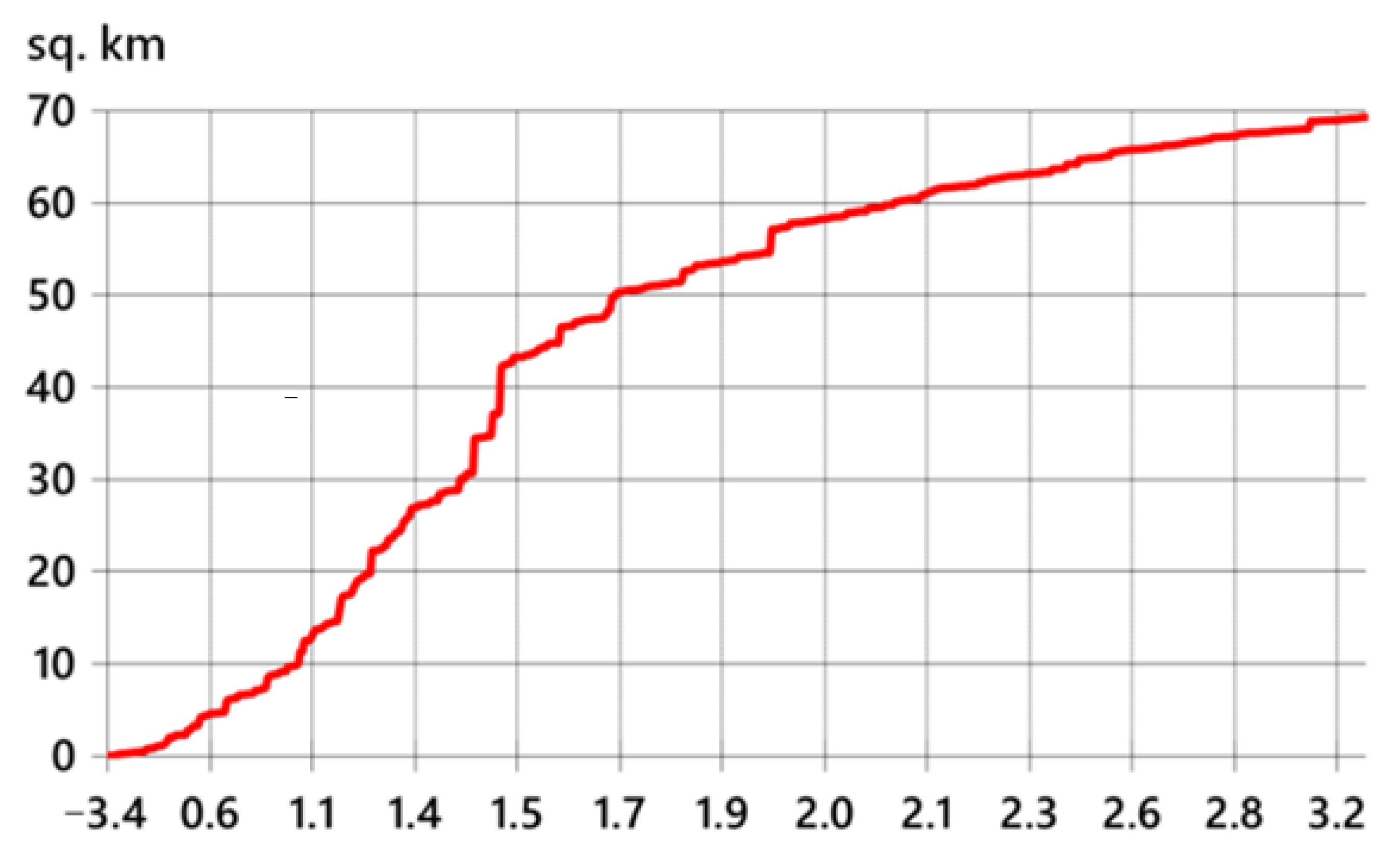
The results of the assessment of the visual attractiveness of geocomplexes (LVA) are presented in Figure 3. The LVA values range from −3.4 (the lowest value) to 4.0 (the highest value). They were grouped into eight classes. The nomenclature (superior, very, moderately, etc.) is conventional and is meant to provide better orientation in the obtained results. Highly attractive areas constitute 3.4% of the study area, very attractive 16.4%, attractive 19.6%, moderately attractive 23.1%, not very attractive 16.4%, unattractive 7.3%, very unattractive 2.4%, and grossly unattractive 3.4%. The three categories with the lowest values correspond to the areas where the negative influence of human activity has marked. The distribution of the index in relation to the study area is shown in Figure 4.
The most visually attractive areas are mainly parts of Pińczów Hummock. The varied relief, entailing a diversity of habitats and vegetation, makes this area exceptionally beautiful and picturesque. The density of borders is the highest here. At the same time, due to the vicinity of Pińczów, devastated areas, garbage dumps, etc., can be found here. The Pińczów Hummock, above the Skowronno Dolne village, is crossed by a high voltage line, which has a particularly adverse effect on the visual attractiveness of the landscape.
The second, also very visually attractive area stretches along the Nida River. It is particularly affected by the presence of water and riverine thickets and bushes (meadows, wicker, reeds). The most attractive areas here are oxbow lakes, where the density of unit boundaries is high.
On Wodzisław Hummock, due to the presence of diverse forests, the attractiveness index is also high. Some of the terrains, located west of the Młodzawy village, are characterized by a high species richness and diversified relief. These places should be taken under special protection (not far from this place lies the nature reserve “Polana Polichno”).
Slightly less attractive visually are the forests and forested areas located on the terraces of the Nida valley. Among them, the most attractive are forests bordering agricultural areas (contrast) and forests on dunes near Skrzypiów village. On the other hand, field areas in the whole study area were considered as average, especially in the flat and monotonous Nida valley, but not lying on the river. In contrast, meadows in the same valley, due to the presence of scrub, are much more attractive.
Overall, the visually unattractive areas are mainly those where the negative impact of human activity is visible. These are mainly areas located in the vicinity of villages, roads, or transmission lines. The most unfavorable influence is exerted on areas used for agricultural purposes, which are characterized by low natural attractiveness index. In many cases, the reduction of visual attractiveness is significant, even by several points. This happens mainly in the vicinity of the Pińczów town and in those units where many electric transmission lines run, e.g., in the vicinity of Zakrzów and Kowala villages.
In this context, the impact of rural development on the aesthetics of the landscape is a concern. Buildings in the area of the Pińczów are particularly neglected; many homesteads are abandoned. Only in about 45% of the assessed units was no adverse human impact found. At the same time, the influence of the location within the landscape park and the resulting legal consequences is practically unnoticeable. It seems necessary not only to observe the existing law in this respect, but also to tighten the regulations (e.g., prohibition of tree felling, individual melioration works). Some areas with the highest aesthetic value should be strictly protected.
3.2. Visibility Analysis
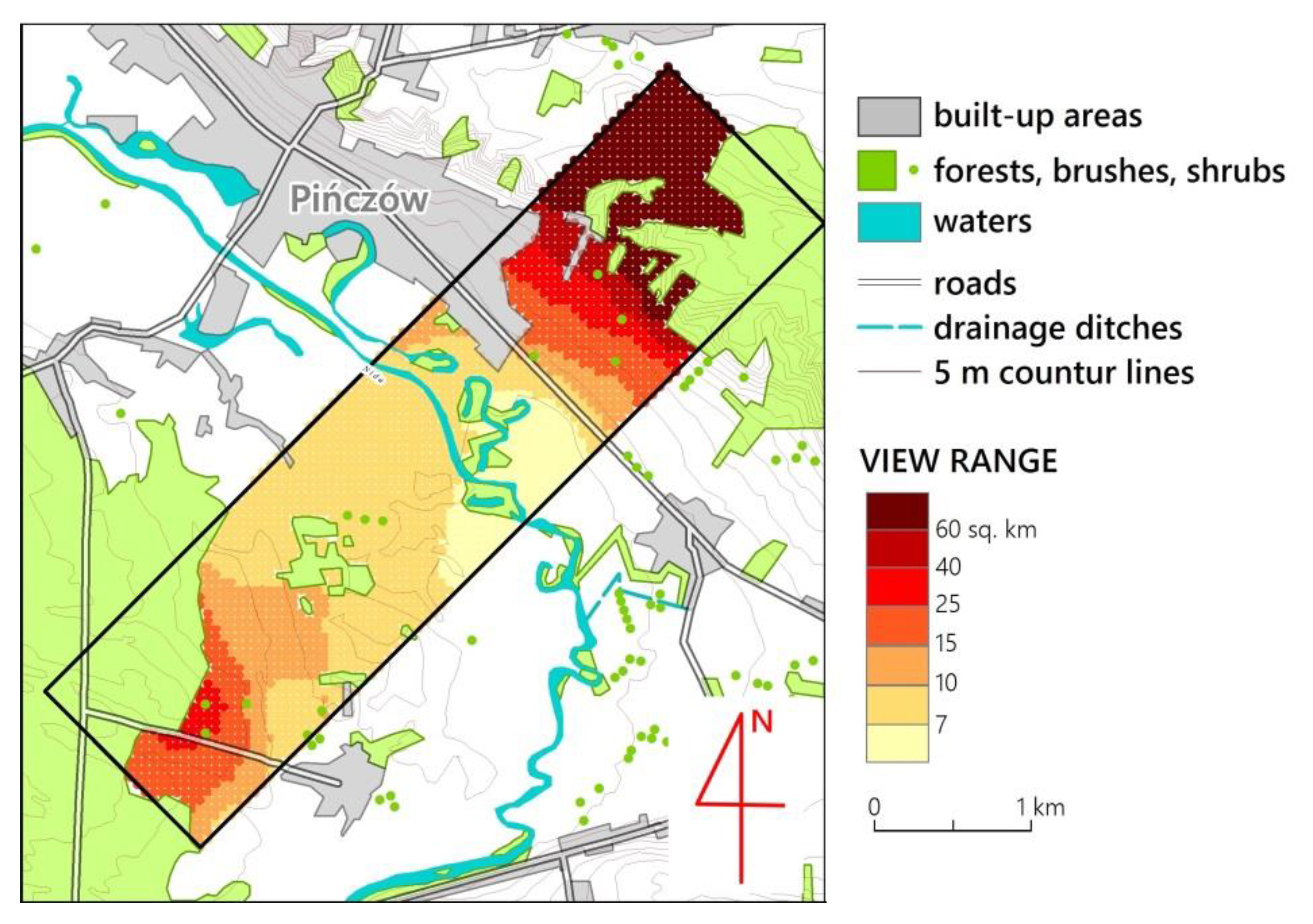
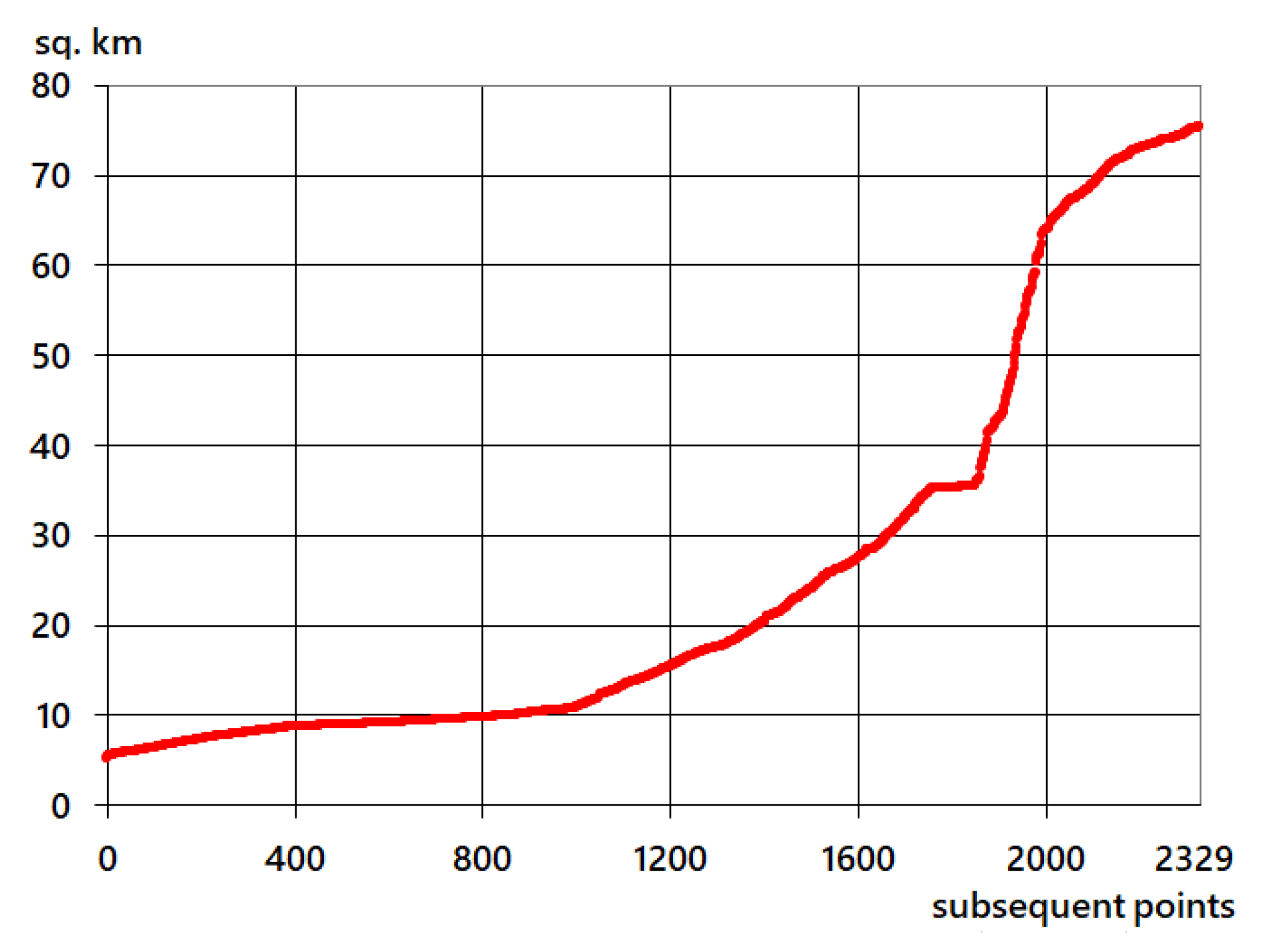
The results of the analysis are presented on the map of the view range (Figure 5) and on the cumulative diagram (Figure 6). According to the calculations, the range of the view is from 5 km2 (the Nida valley) to 75 sq. km (the highest parts of Pińczów Hummock, from which almost the entire study area can be seen). Areas from which the view range is less than 10 km2 constitute 35.8% of the total study area, from 10 to 20 sq. km—15.8%, from 20 to 50 sq. km—8.7%, and above 50 sq. km—12.2%. These values refer only to the study area (77 sq. km). Our own observations suggest that the total extent of the view is greater. For example, from the top parts of the Pińczów Hummock, one can see the hills of the Wodzisław Hummock, located about five kilometers south of the southern border of the study area.
The view range increases with height, and the boundaries of the different view range classes follow the contour of the contour lines to a large extent. This does not mean that individual horizon values relate to the same view isoline values. For example, places from which the view range is about 30 km2 are located in the vicinity of Zakrzów village at an altitude of ca. 195 m and in the vicinity of Pińczów town at an altitude of ca. 205 m.
3.3. Assessment of View-Geocomplexes
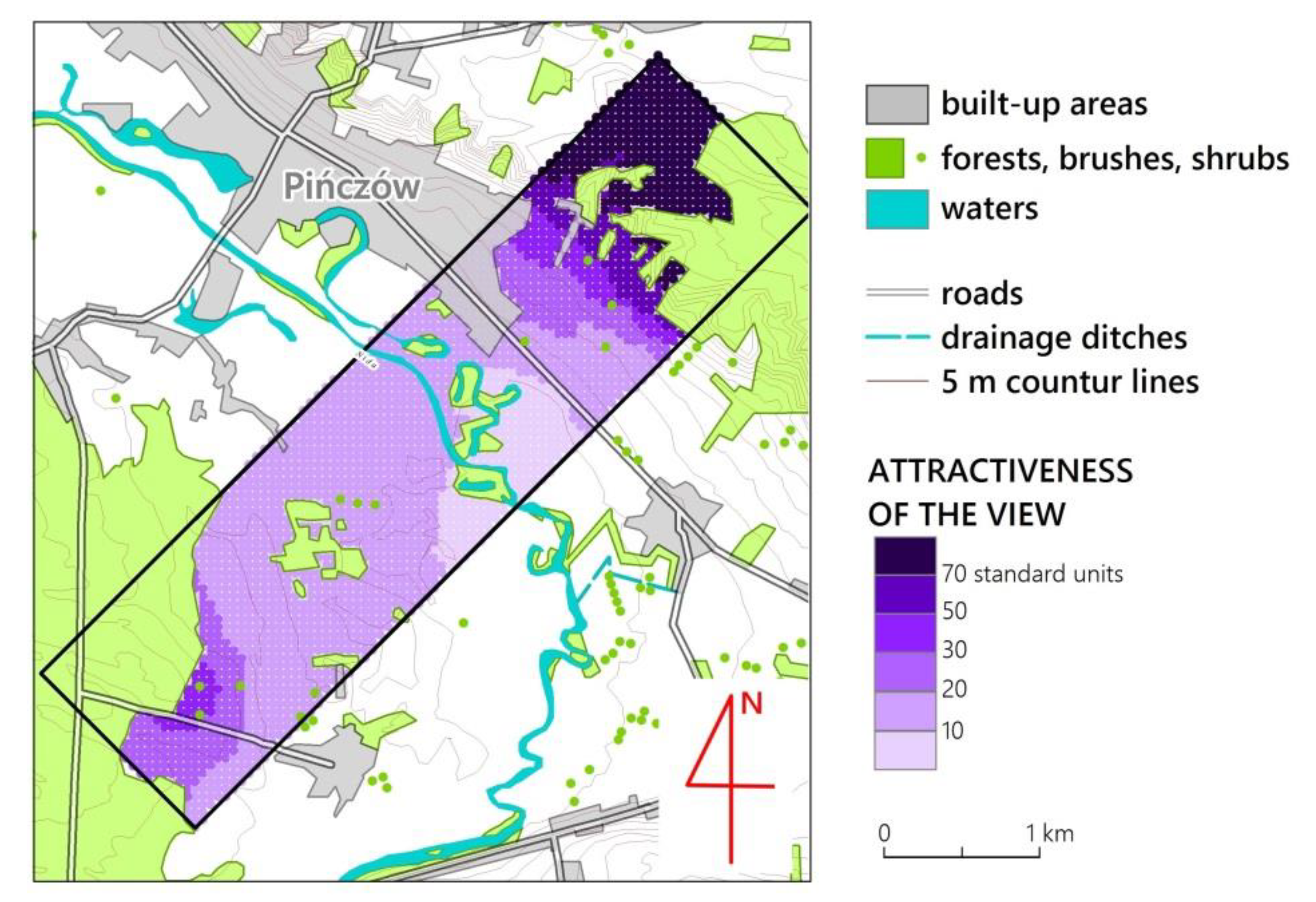
According to the previous assumptions, the attractiveness of the viewsheds is determined by the product of the view-range area and the sum of the visual attractiveness indices of the landscapes (geocomplexes) it contains. Thus, the visual attractiveness map of the view field is the result of combining the maps of view extent (Figure 5) and visual attractiveness of the landscape (Figure 3).
The obtained values of the visual attractiveness index of the view field (Figure 7) were summarized into six classes (Table 7). The areas with the highest view attractiveness represent 7.2%, with very high—31.5%, high—9.4%, average—8.9%, low—3.7%, and the lowest—12.2% of the study area. The values of the index refer to the assumptions stated at the beginning of the chapter that the visual attractiveness of the view field (view attractiveness) is the sum of the products of the sizes of the seen landscape areas and the visual attractiveness indices that characterize them.
The most attractive landscapes stretch from points located on the Pińczów Hummock. These places are also characterized by the largest range of visibility. Quite a high index of attractiveness of the views also characterizes the areas located west of Zakrzów. The diversified Pińczów Hummock is very well visible from these locations. The low value of the landscapes located in the Nida valley was determined primarily by the small range of views.
4. Discussion
The analyses presented here address the hitherto unresolved problem of combining landscape assessment analyses as a geocomplex (territorial unit—ecosystem, catena, region, facies, etc.) with view analyses (viewfield, observation point). As it has been proved, previous attempts to assess landscape visual attractiveness have dealt either with aesthetics (visual attractiveness) of individual landscapes (land surfaces) or views, e.g., view cones. These elements complement each other, and therefore, in a comprehensive assessment of landscape aesthetics (visual attractiveness), not only should both approaches be considered with the help of appropriate methods and tools, specific to a particular group, but attempts should be made to propose such solutions that would combine their properties. Thus, the conducted study of visual attractiveness of a view is an extension of the determination of visual attractiveness of a landscape on the basis of differentiation of physiognomy. This should be regarded as a synthesis of landscape visual attractiveness.
With reference to the objectives of the paper, the discussion of the results was carried out with reference to the different parts of the empirical results, i.e., landscape (geocomplex) assessment, view extent determination and analysis, and landscape assessment in view fields.
The analysis of geocomplexes on the basis of their types determined by superimposing relief and land cover seems to be a satisfactory methodological approach for the assessment of landscape visual attractiveness in the most simple and transparent way. It is quite widely used [13], although there is a very lively discussion about the subjectivity of specific methods [48]. The assessment of geocomplexes for their total area reflects the aesthetic experience of the observer, moving freely in a given type of landscape. Thus, it is a “general” and “bottom-up” assessment [22,23,29]. This method has a great advantage from the point of view of surface nature protection, including the designation of protected landscape areas [49,50], i.e., in Poland national and landscape parks [39,51]. Knowing the average values of landscape types (geocomplexes), they can be transferred (mapped) to another area, and the whole area can be valorized without new surveys. This seems to be quite an important advantage in surveys using photographs. A comparison of the subject and object coverage and the methods used for the different approaches is provided in Table 8.
When determining the extent of a view, it is possible to determine the places from where a given landscape or its element (for example, a river, a peak, a chimney, etc.) can be seen. Moreover, from different locations, the elements filling the landscape can be seen in a different position in relation to each other, which of course also has an impact on further analysis.
The determination of a very detailed grid of points (50 m) proved to be crucial for the reliability of the results. In a relatively diverse landscape, this detail seems to be sufficient, although it is still difficult to find works with such accuracy, especially for Poland [52]. Moreover, since the computation (1996), much effort has been put in by later works to develop faster and more efficient GIS tools related to view line tracking and zooming, reference plane analysis, and view partitioning into blocks [53,54,55,56]. For example, Miller and Law [57] performed an interesting analysis of view structure by building a 3D terrain model and calculating visibility shares of specific land cover types according to Corine Land Cover. More analyses of this type have appeared over time, but they deal almost exclusively with simple analytical operations, particularly related to the visibility of specific features in the field of view. Despite the passage of many years, none of the known studies used more complex analyses, such as the assessment of geocomplex types or landscape diversity itself. For this reason, the method proposed in 1997 and developed in this paper still awaits wider use and further refinement.
The proposed method is also not without its flaws. First, it is based on the assumption that landscape diversity positively influences visual attractiveness and aesthetic value in general. Although there is general agreement on this [13,14,33], in some cases it may not be a valid assumption [48]. Indeed, it is possible to imagine the very high attractiveness of a fairly extensive but very undifferentiated view of, say, a “boundless” desert even from a small dune. Thus, it seems that there are some possibilities to extend the proposed analysis, especially with indicators related to uniqueness and exceptionality.
The disadvantage of the method of assessing landscape visual attractiveness on the basis of physiognomic differentiation is still the relatively high subjectivity of the individual components of the assessment. It seems to be insurmountable [48]. In this, the index of human impact on the environment is particularly subjective. With the progress in the study of human impact on the environment, one should expect an increase in “objectivity” (or, more precisely, “absoluteness”) of this element. At the same time, with the development of landscape diversity studies, further formalization of landscape aesthetic assessment is likely to occur.
The course of action presented in the study, as it seems, can be adopted for other areas as well. It is particularly suitable for use in fairly diverse landscapes and agricultural areas. However, as already mentioned, it requires some refinements, especially in the case of evaluating forest landscapes and determining human influence on the visual attractiveness of the landscape. Still unsolved or poorly solved problems, which require further conceptual–theoretical, methodological search, reconsidering, and empirical work, are:
- -
- A more comprehensive and satisfactory quantification of human impacts (land use, infrastructure, buildings, etc.) on the visual attractiveness of the landscape, not only negative but also positive;
- -
- Investigating the influence of a higher or lower resolution of the grid of points on the results;
- -
- Comparing the influence of the height from which the landscape is seen (important for the design of, e.g., viewing towers, cable cars, and recreational trains);
- -
- Answering the question about the optimal geographical (cartographic) scale for aesthetic landscape assessment, related to human perception, perceptiveness, and usefulness for, e.g., spatial planning;
- -
- Extending the study to other geographical areas, including increasing the physical size of the regions under study (due to a significant increase in computer processing power, this seems feasible);
- -
- examining the usefulness of new databases on the natural environment, which are being created as a result of the development of remote-sensing methods in particular.
In summary, the above analysis of advantages and disadvantages indicates that the proposed method can have a great many applications. The most important advantage is its comparability. The indicators used are universal and can be applied to different types of terrain. It also seems that the system of used indicators (variety of form and content) is exhaustive and can be adopted to more accurate scales of study. On the other hand, smaller scales require the indicators to be expanded (e.g., by adding indicators that characterize colors and details of cover).
5. Summary
In summary, the most important effects obtained are:
- -
- methodological progress in the evaluation of landscape aesthetics and assessment of landscape visual attractiveness, consisting in linking the methods of assessment of geographical units (geocomplexes, micro-regions) with their view from different points;
- -
- proposing detailed criteria and indicators for the above; and
- -
- carrying out the evaluation on a selected example and conclusions for further analyses, which may broaden the research field of landscape evaluation.
Therefore, it seems to be a promising research direction, opening new conceptual and methodological fields in the sphere of landscape aesthetics. In connection with technological (more efficient computers) and geoinformation progress (detailed DTM and land use databases for almost the whole world), the developed algorithm should be tested for other areas and also for other input conditions (e.g., observation height). The next study should also focus on objectifying the impact of human activities (urban layouts, architecture, infrastructure) that may lower or raise the visual value of the landscape.
Research has shown that the Pińczów area has special landscape values. However, their proper use depends largely on the policy of local authorities and the behavior of residents themselves. The presence of high landscape values can contribute to the development of tourism. At the same time the development of tourism should not threaten the landscape values.
The study also proves the special role of landscape aesthetics in shaping the widely understood quality of life. It is hoped that this very important research and practical problem will be continued by geographers.
Supplementary Materials
The following are available online at https://0-www-mdpi-com.brum.beds.ac.uk/2673-7086/1/1/3/s1, Algorithm (operating procedure) for view range calculation and its analysis.
Funding
This research received no external funding.
Institutional Review Board Statement
Not applicable.
Informed Consent Statement
Not applicable.
Data Availability Statement
Local Data Bank of Central Statistical Office of Poland: https://bdl.stat.gov.pl/BDL/start (accessed on 15 January 2021).
Acknowledgments
The author would like to give thanks to Professor Andrzej Richling (University of Warsaw, Faculty of Geography and Regional Studies)—for inspiration and methodological help (the original version of the presented research was the basis for obtaining the Master’s degree in geography in 1996 and for distinguishing the Master’s dissertation in two national professional competitions—first and second place). I would also like to thank other staff of this Faculty, especially the staff of the then Institute of Physico-Geographical Sciences, especially the Department of Geoecology for their above-standard kindness and support. I would like to thank Professor Jerzy Solon (Institute of Geography and Spatial Organization of the Polish Academy of Sciences) for sharing his materials on vegetation of the Pińczów vicinity and biodiversity. I also thank and also Andrzej Jarosz and Tomasz Pecko for writing the source code of the program, calculating the range of the view and its “content”. I would like to thank Professor Tadeusz J. Chmielewski for his valuable guidance in the field of newer literature.
Conflicts of Interest
The author declare no conflict of interest.
References
- Śleszyński, P. From the research on natural environment physiognomy. Prace i Studia Geograficzne 1997, 21, 255–297. [Google Scholar]
- Linton, D.L. The assessment of scenery as a natural resource. Scott. Geogr. Mag. 1968, 84, 219–238. [Google Scholar] [CrossRef]
- Geikie, A. The Scenery of Scotland; Macmillan and Co.: London, UK, 1901. [Google Scholar]
- Bailey, E.B. The Interpretation of Scottish Scenery. Scott. Geogr. Mag. 1934, 50, 308–330. [Google Scholar] [CrossRef]
- Kühne, O. Landscape Theories. A Brief Introduction. In RaumFragen: Stadt-Region-Landschaft Book Series; Springer VS: Wiesbaden, Germany, 2019. [Google Scholar] [CrossRef]
- Hepburn, R.W. Contemporary Aesthetics and the Neglect of Natural Beauty. In British Analytical Philosophy; Williams, B., Montefiore, A., Eds.; Routledge: London, UK, 1966; pp. 225–241. [Google Scholar]
- De Groot, R. Function-analysis and valuation as a tool to assess land use conflicts in planning for sustainable, multi-functional landscapes. Landsc. Urban Plan. 2006, 75, 175–186. [Google Scholar] [CrossRef]
- Termorshuizen, J.W.; Opdam, P. Landscape services as a bridge between landscape ecology and sustainable development. Landsc. Ecol. 2009, 24, 1037–1052. [Google Scholar] [CrossRef]
- Sahraoui, Y.; Clauzel, C.; Foltête, J.-C. A metrics-based approach for modeling covariation of visual and ecological landscape qualities. Ecol. Indic. 2021, 123, 107331. [Google Scholar] [CrossRef]
- Dupont, L.; Antrop, M.; Van Eetvelde, V. Does landscape related expertise influence the visual perception of landscape photographs? Implications for participatory landscape planning and management. Landsc. Urban Plan. 2015, 141, 68–77. [Google Scholar] [CrossRef] [Green Version]
- Tveit, M.S.; Ode Sang, Å.; Hagerhall, C.M. Scenic Beauty. In Environmental Psychology; Steg, L., Groot, J.I.M., Eds.; Wiley: Hoboken, NJ, USA, 2018. [Google Scholar] [CrossRef]
- Ioannidis, R.; Koutsoyiannis, D. A review of land use, visibility and public perception of renewable energy in the context of landscape impact. Appl. Energy 2020, 276, 115367. [Google Scholar] [CrossRef]
- Zube, E.H.; Sell, J.L.; Taylor, J.G. Landscape perception: Research, application and theory. Landsc. Plan. 1982, 9, 1–33. [Google Scholar] [CrossRef]
- Nasar, J.L. (Ed.) Environmental Aesthetics: Theory, Research, and Application; Cambridge University Press: Cambridge, UK, 1988. [Google Scholar]
- Porteous, J.D. Environmental Aesthetics: Ideas, Politics and Planning; Routledge: New York, NY, USA; Abingdon, UK, 1996. [Google Scholar]
- Wagner, V.L. John Ruskin and Artistical Geology in America. Winterthur Portf. 1988, 23, 151–167. [Google Scholar] [CrossRef]
- Brossard, T.; Wieber, J.-L. Le Paysage: Trois définitions, un mode d’analyse et de cartographie. Lespace Géographique 1984, 13, 5–12. [Google Scholar] [CrossRef]
- Vukomanovic, J.; Orr, B.J. Landscape Aesthetics and the Scenic Drivers of Amenity Migration in the New West: Naturalness, Visual Scale, and Complexity. Land 2014, 3, 390–413. [Google Scholar] [CrossRef] [Green Version]
- Migoń, P. Granite Landscapes, Geodiversity and Geoheritage—Global Context. Heritage 2021, 4, 198–219. [Google Scholar] [CrossRef]
- Sobala, M.; Pukowiec-Kurda, K.; Żemła-Siesicka, A. The Delimitation of Landscape Units for the Planning of Protection—The Example of the Forests by Upper Liswarta Landscape Park. Quaestiones Geographicae 2019, 38, 97–105. [Google Scholar] [CrossRef] [Green Version]
- Kowalczyk, A. The Iconic Model of Landscape Aesthetic Value. Eur. Spat. Res. Policy 2012, 19, 121–128. [Google Scholar] [CrossRef] [Green Version]
- Bishop, I.D. Assessment of visual qualities, impacts, and behaviours, in the landscape, by using measures of visibility. Environ. Plan. B Plan. Des. 2003, 30, 677–688. [Google Scholar] [CrossRef]
- Tveit, M.; Ode, Å.; Fry, G. Key concepts in a framework for analysing visual landscape character. Landsc. Res. 2006, 31, 229–255. [Google Scholar] [CrossRef]
- Chen, Y.; Sun, B.; Liao, S.B.; Chen, L.; Luo, S.X. Landscape perception based on personal attributes in determining the scenic beauty of in-stand natural secondary forests. Ann. For. Res. 2016, 59, 91–103. [Google Scholar] [CrossRef] [Green Version]
- Le, Q.-T.; Ladret, P.; Nguyen, H.-T.; Caplier, A. Image Aesthetic Assessment Based on Image Classification and Region Segmentation. J. Imaging 2021, 7, 3. [Google Scholar] [CrossRef]
- Frank, S.; Fürst, C.; Koschke, L.; Witta, A.; Makeschina, F. Assessment of landscape aesthetics—Validation of a landscape metrics-based assessment by visual estimation of the scenic beauty. Ecol. Indic. 2013, 32, 222–231. [Google Scholar] [CrossRef]
- Chmielewski, S. Chaos in Motion: Measuring Visual Pollution with Tangential View Landscape Metrics. Land 2020, 9, 515. [Google Scholar] [CrossRef]
- Arriaza, M.; Canas-Ortega, J.F.; Canas-Madueno, J.A.; Ruiz-Aviles, P. Assessing the visual quality of rural landscapes. Landsc. Urban Plan. 2004, 69, 115–125. [Google Scholar] [CrossRef]
- Daniel, T.C.; Vining, J. Methodological Issues in the Assessment of Landscape Quality. In Behavior and the Natural Environment. Human Behavior and Environment; Altman, I., Wohlwill, J.F., Eds.; Advances in Theory and Research, 6; Springer: Boston, MA, USA, 2019; pp. 39–84. [Google Scholar] [CrossRef]
- Palmer, J.F. Using spatial metrics to predict scenic perception in a changing landscape: Dennis, Massachusetts. Landsc. Urban Plan. 2004, 69, 201–218. [Google Scholar] [CrossRef]
- Chien, Y.-M.C.; Carver, S.; Comber, A. Using geographically weighted models to explore how crowdsourced landscape perceptions relate to landscape physical characteristics. Landsc. Urban Plan. 2020, 203, 103904. [Google Scholar] [CrossRef]
- Hermes, J.; Albert, C.; von Haaren, C. Assessing the aesthetic quality of landscapes in Germany. Ecosyst. Serv. 2018, 31, 296–307. [Google Scholar] [CrossRef]
- Carlson, A. Nature and Landscape: An Introduction to Environmental Aesthetics; Columbia University Press: New York, NY, USA, 2009. [Google Scholar]
- Barsch, H. Arbeitsmethoden in der Landschaftsökologie. In Arbeitsmethoden in der Physischen Geographie; Heyer, E., Ed.; Gotha Stuttgart Klett-Perthes: Berlin, Germany, 1968; pp. 235–273. [Google Scholar]
- Shary, P.A.; Sharaya, L.S.; Mitusov, A.V. Fundamental quantitative methods of land surface analysis. Geoderma 2002, 107, 1–32. [Google Scholar] [CrossRef]
- Washtell, J.; Carver, S.; Arrell, K. A viewshed based classification of landscapes using geomorphometrics. In Proceedings of the Geomorphometry Conferences, Zurich, Switzerland, 31 August–2 September 2009; pp. 44–49. [Google Scholar]
- Śleszyński, P. A geomorphometric analysis of Poland on the basis of SRTM-3 data. Geogr. Pol. 2012, 85, 47–61. [Google Scholar] [CrossRef] [Green Version]
- Chmielewski, T.J.; Butler, A.; Kułak, A.; Chmielewski, S. Landscape’s physiognomic structure: Conceptual development and practical applications. Landsc. Res. 2018, 43, 410–427. [Google Scholar] [CrossRef]
- Chmielewski, T.J.; Solon, J. Basic natural spatial units of the Kampinoski National Park: Rules of delineation and ways of protection. Probl. Landsc. Ecol. 1996, 2, 130–142. [Google Scholar]
- Michalik-Śnieżek, M.; Chmielewski, S.; Chmielewski, T.J. An introduction to the classification of the physiognomic landscape types: Methodology and results of testing in the area of Kazimierz Landscape Park (Poland). Phys. Geogr. 2019, 40, 384–404. [Google Scholar] [CrossRef]
- Ostręga, A.; Cała, M. Assessing the value of landscape shaped by the mining industry—A case study of the town of Rydułtowy, Poland. Arch. Min. Sci. 2020, 65, 3–18. [Google Scholar] [CrossRef]
- Solon, J.; Borzyszkowski, J.; Bidłasik, M.; Richling, A.; Badora, K.; Balon, J.; Brzezińska-Wójcik, T.; Chabudziński, Ł.; Dobrowolski, R.; Grzegorczyk, I.; et al. Physico-geographical mesoregions of Poland: Verification and adjustment of boundaries on the basis of contemporary spatial data. Geogr. Pol. 2018, 91, 143–170. [Google Scholar] [CrossRef]
- Kondracki, J. (Ed.) Geographical studies on the Pińczów district. In Prace Geograficzne, 45; Institute of Geography of Polish Academy of Sciences: Warsaw, Poland, 1966. [Google Scholar]
- Kostrowicki, J.; Solon, J. (Eds.) Geobotanical and landscape case-study in Pinczów areas. In Dokumentacja Geograficzna, 1-2; Institute of Geography and Spatial Organization of Polish Academy of Sciences: Warsaw, Poland, 1994. [Google Scholar]
- Stopa-Boryczka, M.; Bogacki, M. (Eds.) Geographical Studies of Ponidzie Pińczowskie. In Prace i Studia Geograficzne, 27; Faculty of Geography and Regional Studies of University of Warsaw: Warsaw, Poland, 2000. [Google Scholar]
- Amidon, E.L.; Elsner, G.H. Delineating Landscape View Areas—A Computer Approach; Research Note, PSW-180; U.S.O.A. Forest Service: Boise, ID, USA, 1968.
- Śleszyński, P. Visibility range map of Pińczów vicinity. Pol. Przegląd Kartogr. 1998, 30, 173–184. [Google Scholar]
- Ribe, R.G. Can Professional Aesthetic Landscape Assessments Become More Truly Robust? Challenges, Opportunities, and a Model of Landscape Appraisal. In Visual Resource Stewardship Conference Proceedings: Landscape and Seascape Management in a Time of Change; Gobster, P.H., Smardon, R.C., Eds.; General Technical Report, NRS-P-183; U.S. Department of Agriculture, Forest Service, Northern Research Station: Newtown Square, PA, USA, 2018; pp. 44–56. [Google Scholar]
- Brooks, R.O.; Lavigne, P. Aesthetic theory and landscape protection: The many meanings of beauty and their implications for the design, control and protection of Vermont’s landscape. UCLA J. Environ. Law Policy 1985, 2, 129–172. [Google Scholar]
- Lange, E.; Bishop, I. Our Visual Landscape: Analysis, modeling, visualization and protection. Landsc. Urban Plan. 2001, 54, 1–3. [Google Scholar] [CrossRef]
- Chmielewski, T.J.; Kułak, A.; Michalik-Śnieżek, M.; Lorens, B. Physiognomic structure of agro-forestry landscapes: Method of evaluation and guidelines for design, on the example of the West Polesie Biosphere Reserve. Int. Agrophysics 2016, 30, 415–429. [Google Scholar] [CrossRef]
- Nita, J.; Myga-Piątek, U. Scenic Values of The Katowice-Częstochowa Section of National Road No. 1. Geogr. Pol. 2014, 87, 113–125. [Google Scholar] [CrossRef] [Green Version]
- Sobala, M.; Myga-Piątek, U.; Szypuła, B. Assessment of Changes in a Viewshed in the Western Carpathians Landscape as a Result of Reforestation. Land 2020, 9, 430. [Google Scholar] [CrossRef]
- Wu, H.; Pan, M.; Yao, L.; Luo, B. A partition-based serial algorithm for generating viewshed on massive DEMs. Int. J. Geogr. Inf. Sci. 2007, 21, 955–964. [Google Scholar] [CrossRef]
- Roth, M.; Gruehn, D. Visual Landscape Assessment for Large Areas-Using GIS, Internet Surveys and Statistical Methodologies. Proc. Latv. Acad. Sci. Sect. A Humanit. Soc. Sci. 2012, 66, 129–142. [Google Scholar]
- Wang, Y.; Dou, W. A fast candidate viewpoints filtering algorithm for multiple viewshed site planning. Int. J. Geogr. Inf. Sci. 2020, 34, 448–463. [Google Scholar] [CrossRef]
- Miller, D.R.; Law, A.N.R. The mapping of terrain visibility. Cartogr. J. 1997, 34, 87–91. [Google Scholar] [CrossRef]
Figure 1.
Study area. Source: own elaboration based on based on IGSO PAS digital databases.

Figure 2.
Geocomplexes mapped in the study area. Source: Author’s delimitation based on unpublished geomorphological and phytosociological materials in the archives of the Faculty of Geography and Regional Studies, University of Warsaw.
Figure 2.
Geocomplexes mapped in the study area. Source: Author’s delimitation based on unpublished geomorphological and phytosociological materials in the archives of the Faculty of Geography and Regional Studies, University of Warsaw.

Figure 3.
Assessment of the visual attractiveness of landscapes (geocomplexes). Source: own elaboration.
Figure 3.
Assessment of the visual attractiveness of landscapes (geocomplexes). Source: own elaboration.

Figure 4.
Increase of landscape visual attractiveness index (horizontal axis) in dependence on the sum of unit areas (vertical axis). Source: own elaboration.
Figure 4.
Increase of landscape visual attractiveness index (horizontal axis) in dependence on the sum of unit areas (vertical axis). Source: own elaboration.

Figure 5.
Range of view delineated from 2329 points in the study area. Source: own elaboration

Figure 6.
Distribution of view range values for individual points in the study area. Source: own elaboration.
Figure 6.
Distribution of view range values for individual points in the study area. Source: own elaboration.

Figure 7.
Assessment of view attractiveness. Source: own elaboration


Table 1.
Number of basic units (geocomplexes) by selected types of relief and land use.
| Land Use (Vegeta-Tion) Relief | Arable Land | Moist Meadows and Pastures | Grasslands and Dry Meadows | Bushes, Shrubs | Pine Stands | Pine Forests | Larch Forests | Broad-Leaved Forests | Total |
|---|---|---|---|---|---|---|---|---|---|
| Valley bottoms | 11 | 13 | - | 43 | - | - | - | - | 67 |
| Overflood terraces | 25 | 13 | - | 8 | 5 | 4 | 2 | 56 | |
| Terrace plains | 34 | 7 | - | 12 | 5 | 8 | 5 | 2 | 73 |
| Terrace monadnocks | 1 | 1 | - | 1 | - | - | - | - | 3 |
| Wind-blown sandy areas | 9 | 3 | 5 | 1 | 9 | 1 | 2 | 30 | |
| Planation surfaces | 21 | 2 | 3 | 3 | 1 | 1 | 1 | 3 | 35 |
| Low-gradient hillslopes | 54 | 4 | 4 | 8 | 5 | 14 | 2 | 6 | 97 |
| High-gradient hillslopes | 35 | 22 | 7 | 8 | 2 | 3 | 78 | ||
| Dry valleys and gullies | 75 | 15 | 19 | 11 | 2 | 23 | 5 | 8 | 158 |
| Total | 264 | 56 | 62 | 88 | 19 | 65 | 15 | 25 | 597 |
Source: own study (Tables 1–7).
Table 2.
The detailed indicator values used.
| Indicator | Quantitative and Qualitative Identification (Criteria) | |
|---|---|---|
| Form diversity (DF) | ||
| Da | area diversity | ratio of circumference to area (L/A, where L–circumference of the unit, A–area) |
| Dc | contrast diversity between landscapes | see Table 3 |
| Content (body matter) diversity (DB) | ||
| Dr | vertical diversity of the relief | based on the ratio of the length of the contour lines to the area, see Table 4 |
| Dv | vertical variation of vegetation (land cover) | height of the vegetation layer (see Table 5) |
| Dd | typological richness of vegetation | number of species (genera or other taxon), see Table 5 |
| H–negative impact of human activity (see Table 6) | ||
Table 3.
Boundary contrast index values for each coverage type.
| Waters | Forests | Bushes, Shrubs | Arable Land | Meadows and Pastures | |
|---|---|---|---|---|---|
| Waters | 0 | non-existent | 5 | 4 | 4 |
| Forests | non-existent | 0 | 2 | 5 | 5 |
| Bushes, shrubs | 5 | 2 | 0 | 3 | 2 |
| Arable land | 4 | 5 | 3 | 0 | 5 |
| Meadows and pastures | 4 | 5 | 2 | 2 | 0 |
Notice: indicator value for other borders = 1.
Table 4.
Values of the index of vertical extension of relief (vertical differentiation).
| Type of relief | Generalized Index Value |
|---|---|
| Valley bottoms | 1.0 |
| Overflood terraces | 2.0 |
| Terrace plains | 4.0 |
| Terrace monadnocks | 2.0 |
| Wind-blown sandy areas | 3.0 |
| Planation surfaces | 2.0 |
| Low-gradient hillslopes | 3.0 |
| High-gradient hillslopes | 5.0 |
| Dry valleys and gullies – on the Pińczów Hummock – others | 5.0 4.0 |
Table 5.
Values of the vertical extent of coverage (vertical diversity) and richness indices.
| Type of Land Cover (Vegetation) | Vertical Differentiation | Typological Richness of the Vascular Flora * | ||
|---|---|---|---|---|
| Height of Vege-Tation Layer (m) | Value of Indicator | Number of Genera/Species | Value of Indicator | |
| Arable land | 0.6–1.7 * | 1.5 | 3–5 | 1.0 |
| Moist meadows and pastures | 0.1–1.0 * | 1.0 | 10–20 | 3.0 |
| Grasslands and dry meadows | 0.1–1.0 * | 1.0 | 20–30 | 5.0 |
| Bushes, shrubs | 1.0–2.5 * | 2.5 | 15–25 | 4.0 |
| Pine stands | 1.0–4.0 | 3.0 | 3–5 | 1.0 |
| Pine forests | >6.0 | 5.0 | 10–15 | 2.0 |
| Larch forests | >6.0 | 5.0 | 3–5 | 1.0 |
| Broad-leaved forests | >6.0 | 5.0 | 20–30 | 5.0 |
* during the summer.
Table 6.
Adverse human impact index values adopted in the study area.
| Object (Element of Assessment) | Indicator Value |
|---|---|
| Road with hardened surface: – for each 100 m of road running or bordering a unit per 0.5 sq. km of that unit’s area | −5 |
| Transmission line: – for each 100 m of aboveground transmission, telephone or telegraph line running or bordering a unit per 0.5 sq. km of area of that unit | −3 |
| Small point features (facilities): landfill, wild dump, small pit, other small infrastructure features (switching stations, abandoned warehouses): – for each such facility per 0.1 sq. km of the unit area | −5 |
| Boundary with built-up area: for each 1/5 of the length of the common boundary with an area: – urban – rural | −2 −1 |
Table 7.
Characteristics of view attractiveness in the study area.
| Areas with Attractive Views | Indicator Values | Number of Visible Points | Area (sq. km) | Share (%) |
|---|---|---|---|---|
| Highest | 51–78 | 231 | 0.58 | 7.2 |
| Very high | 31–50 | 1007 | 2.52 | 31.5 |
| High | 21–30 | 300 | 0.75 | 9.4 |
| Average | 16–20 | 285 | 0.71 | 8.9 |
| Small | 11–15 | 117 | 0.29 | 3.7 |
| Least | 5–10 | 389 | 0.97 | 12.2 |
| Buildings, forests, and water (points not taken into account in these areas) | – | 912 | 2.28 | 28.5 |
| Total | – | 3241 | 8.00 | 100.0 |
Table 8.
The comparison of the subject and problem scopes and methods used in different approaches to assessing the visual and aesthetic attractiveness of landscapes.
Table 8.
The comparison of the subject and problem scopes and methods used in different approaches to assessing the visual and aesthetic attractiveness of landscapes.
| Characteristic | Psycho-Sociological (Behavioral) Research into Landscape Preferences | Psycho-Sociological (Behavioral) Research into Landscape Preferences | Assessment of Views (e.g., from Vantage Points, Traffic Routes) | The Proposed Method |
|---|---|---|---|---|
| Spatial unit of reference | field of vision, frame, visible fragment of space | field of vision, frame, visible fragment of space | field of view, cone of view | total field of view |
| Source material | observer’s stay in the field, photography, film | observer’s stay in the field, photography, film | DTM, data on land cover, infrastructure, buildings, etc. | secondary data (and own calculation of field of view) |
| Methods used | quantitative and qualitative methods: experiment, interview (survey, questionnaire interview) | quantitative and qualitative methods: experiment, interview (survey, questionnaire interview) | spatial analysis, classification, indicator method | index method |
| Possibility to introduce a spatio-temporal variable (time of day, time of year, weather, visibility conditions) | yes | yes | limited | very limited |
| Possibility to assess the same landscape from different locations | yes, arbitrary, although limited by human perception of a certain number of photos | yes, arbitrary, although limited by human perception of a certain number of photos | yes, e.g., from different angles, “from below” and “from above | only from one position (“from above” or “from below”), depending on the location of the point in the grid. Potentially great opportunities due to GIS development (e.g., evaluation of the same area containing different landscapes/geocomplexes) seen from different locations) |
| Comparability of assessment for different areas (repeatability) | weak (same landscape types differ in different places e.g., share of borders with the same contrast) | weak (same landscape types differ in different places e.g., share of borders with the same contrast) | low | high |
| Subjectivity of the assessment | high (in the sense of assessment of a single observer), low (in the sense of averaging of representative results) | high (in the sense of assessment of a single observer), low (in the sense of averaging of representative results) | very high, great difficulty to objectivize the assessment of the view field (due to complex topology of plans) | moderate, as numerous and regular measurements eliminate the problem of selection and representativeness |
| Usefulness for practical purposes, e.g., spatial planning, environmental protection, conservation of historical monuments | varied | varied | good for local scales and urban design | high for local scales, other scales need checking |
Publisher’s Note: MDPI stays neutral with regard to jurisdictional claims in published maps and institutional affiliations. |
© 2021 by the author. Licensee MDPI, Basel, Switzerland. This article is an open access article distributed under the terms and conditions of the Creative Commons Attribution (CC BY) license (http://creativecommons.org/licenses/by/4.0/).
Share and Cite
MDPI and ACS Style
Śleszyński, P. Multi-Item Assessment of Physiognomic Diversity of Geocomplexes as a Comprehensive Method of Visual-Aesthetic Landscape Assessment. Geographies 2021, 1, 22-46. https://0-doi-org.brum.beds.ac.uk/10.3390/geographies1010003
AMA Style
Śleszyński P. Multi-Item Assessment of Physiognomic Diversity of Geocomplexes as a Comprehensive Method of Visual-Aesthetic Landscape Assessment. Geographies. 2021; 1(1):22-46. https://0-doi-org.brum.beds.ac.uk/10.3390/geographies1010003
Chicago/Turabian StyleŚleszyński, Przemysław. 2021. "Multi-Item Assessment of Physiognomic Diversity of Geocomplexes as a Comprehensive Method of Visual-Aesthetic Landscape Assessment" Geographies 1, no. 1: 22-46. https://0-doi-org.brum.beds.ac.uk/10.3390/geographies1010003