Technical Note

Spatiotemporal Land-Use Changes of Batticaloa Municipal Council in Sri Lanka from 1990 to 2030 Using Land Change Modeler

by
Ibra Lebbe Mohamed Zahir
1,*,
Sunethra Thennakoon
2,
Rev. Pinnawala Sangasumana
2,
Jayani Herath
2,
Buddhika Madurapperuma
3 and
Atham Lebbe Iyoob
4
1
Department of Geography, South Eastern University of Sri Lanka, University Park, Oluvil 32360, Sri Lanka
2
Department of Geography, University of Sri Jayewardenepura, Gangodawila, Nugegoda 10250, Sri Lanka
3
Department of Forestry and Wildland Resources, Humboldt State University, 1st Harpst Street, Arcata, CA 95521, USA
4
Land Use Policy Planning Department, District Secretariat, Ampara 32000, Sri Lanka
*
Author to whom correspondence should be addressed.
Submission received: 2 September 2021 / Revised: 22 September 2021 / Accepted: 23 September 2021 / Published: 28 September 2021
(This article belongs to the Special Issue Early Career Scientists’ (ECS) Contributions to Geographies)

Abstract

:
Land-use change is a predictable and principal driving force of potential environmental changes on all spatial and temporal scales. A land-use change model is a tool that supports the analysis of the sources and consequences of land-use dynamics. This study aims to assess the spatiotemporal land-use changes that occurred during 1990–2020 in the municipal council limits of Batticaloa. A land change modeler has been used as an innovative land planning and decision support system in this study. The main satellite data were retrieved from Landsat in 1990, 2000, 2010, and 2020. For classification, the supervised classification method was employed, particularly with the medium resolution satellite images. Land-use classes were analyzed by the machine learning algorithm in theland change modeler. The Markov chain method was also used to predict future land-use changes. The results of the study reveal that only one land-use type, homestead, has gradually increased, from 12.1% to 34.1%, during the above-mentioned period. Agriculture land use substantially declined from 26.9% to 21.9%. Bare lands decreased from 11.5% to 5.0%, and wetlands declined from 13.9% to 9.6%.

Graphical Abstract

1. Introduction

The term land-use refers to the system of how the land is being used and influencedby human activities for different needs. It forms a direct link between land-use and land-cover, and the action of the people in the environment [1]. The dynamics of land-use are of great concern on the Earth’s surface [2]. Significant changes in land-use cause a constant strain on the ecology [3,4,5]. Generally, anthropogenic activities in land-use have been accepted as significant factors in global change [6,7,8]. These changes have been reviewed as the critical driving forces of ecological change on all spatial and temporal scales [9]. Environmental issues have attracted the attention of the people of the world and they are now becoming increasingly conscious of a variety of environmental challenges to well-being by unplanned urban development. Therefore, current environmental problems can be classified into three parts in urban centers: the problems arising from, and associated with, poverty and underdevelopment; the problems arising as the negative effects of every process of development; and the problems related to man-made pollution.
Land-use change is not static because of dynamic and continuous processes [10]. Monitoring of these changes is needed overall in environmental and ecosystem services [11]. Geographical information systems (GISs) and remote sensing technology platforms that monitor the temporal changes of land-use have become the most effective methods possible, at a low-cost and with better accuracy for data analysis, update, and retrieval [12,13,14]. Landsat remote sensing data have provided valuable and continuous information about the Earth’s landscape for approximately the past four decades. The archive of this series of data is now made freely available for scientific decision-making and, thus, it serves as a repertoire of information for identifying and monitoring the changes imposed on the physical and human environment [15]. Remote sensing data is the most important for application and is widely used forupdating land-use change maps [16]. At present, cities are growing twice as fast because of rapid population growth [17]. Consequently, this indicates that changes in urban land-use could produce a near tripling in the global urban land in the future, adding hundreds of thousands of additional square kilometers to urban levels of density [17]. Such urban expansions threaten to destroy ecosystem habitats and contribute to the carbon emissions associated with tropical deforestation and land-use change [18]. Nowadays, Earth resource satellite data are useful for estimating land-use change and detection analysis [16,19]. Land-use change has been applied in numerous studies in the spatially apparent scientific field [6,20].
The land change modeler (LCM) is an estimating and predicting process that determines land-use change [21]. The LCM is a simplification of reality that offers an important means of predicting the weight of land-use change [22,23]. The analysis of land-use change has produced a strong model by integrating multilayer perception in the LMC process in raster data form between land-use classes [5,6,24,25,26,27]. These models reflect the dynamic changes in land-use over time. However, land-use might be static during a short time. Therefore, a Markov chain model can be used to predict the process from past to future [7]. Many scholars have widely used this model on land-use changes, including on both urban and nonurban areas, for large spatiotemporal scales [23,24,25,26,27,28]. The Markov chain model was applied for sustainable land demand in recent urban studies [2,17,29]. On the basis of this concept, the model might apply to regions that experience rapid land-use change. Land-use has been changing because of the inappropriate processes of the administrative area of theBatticaloa Municipal Council (BMC). However, a few studies have been applied to assess land-use changes through the spatial analysis concept. These concepts are not good enough to utilize the land for forthcoming purposes in effective ways. The empirical land-use and Markov chain model were employed to simulate the land-use change in the present study. The main objective of the study is to measure the land-use changes that have occurred in the BMC during the last thirty years.
We address the following research questions:
  • What is the extent and magnitude of land-use change in the BMC from 1990 to 2020?
  • What are the primary drivers of land-use change in the BMC?
  • How do historic land-use changes differ from simulated land-uses in the BMC?
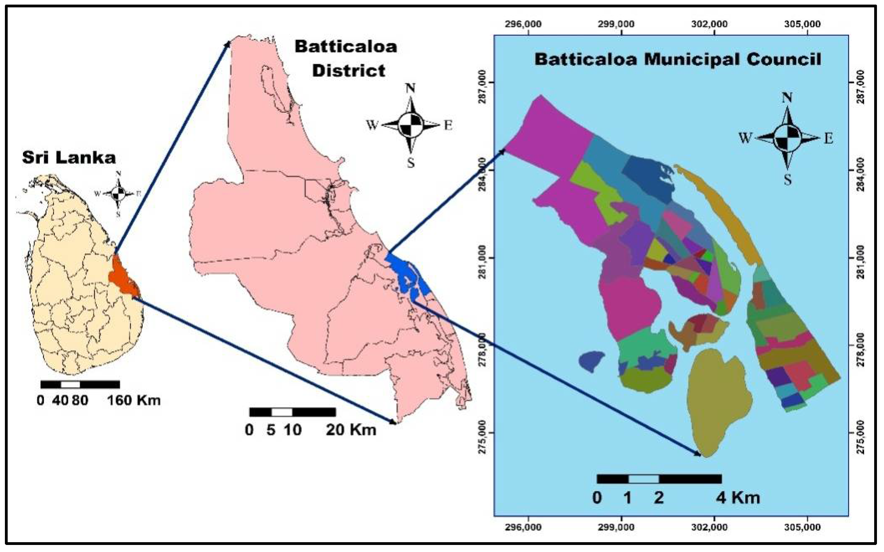
2. Study Area

The study area is laid between north of 7°39′53″ to 7°44′36″ and 81°39′17″ to 81°41′54″ on the east, in the central part of the Eastern Province of Sri Lanka. The BMC is divided into forty-eight (48) GNDs (Figure 1), which consist of some parts of the suburb. The study consists of an area of about 4570.6 ha. The mean annual rainfall and temperature are 1500 mm and range from 28 °C to 34 °C, respectively [30]. In the BMC, remarkable changes in land-use are observed due to urban development and the rapidly increasing population. The rapid development of sectors, such as the residential, commercial, industrial, service, and recreational sectors, has been improved by the utilization of land. This has revealed the changes in land-use in the spatial domain. Therefore, it is important to monitor land-use changes when considering the existing scenario, forecasting future change, and planning for the future development of the urban area. The latest geospatial technology is necessary to simulate contemporary and projected land-use changes for the BMC.
The study area has faced challenges to land-use by the civil war, a rapidly increasing population, and anthropogenic activities. Moreover, the lack of proper land-use guidelines has led to temporal land-use changes and conflictsaround land-use. According to Mathanraj et al. [31], the growth of the city without proper planning leads to the creation of many complex problems. The population growth exploited agricultural land and other land areas. The overcrowding of the population directly affected the other land areas. The correlation relationship is significant between population growth and land-use change in the BMC [31].

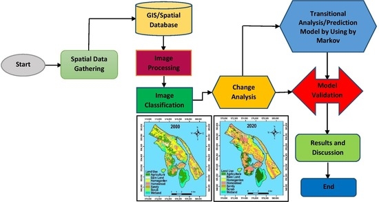
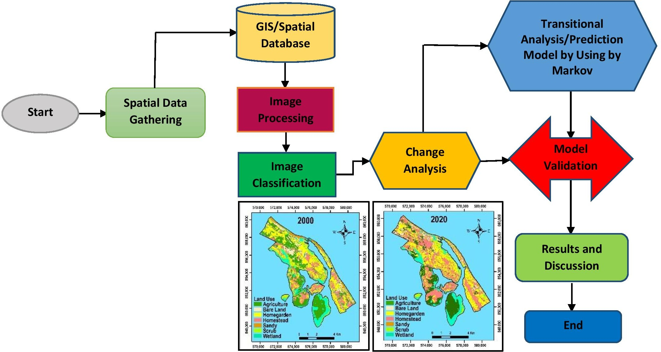
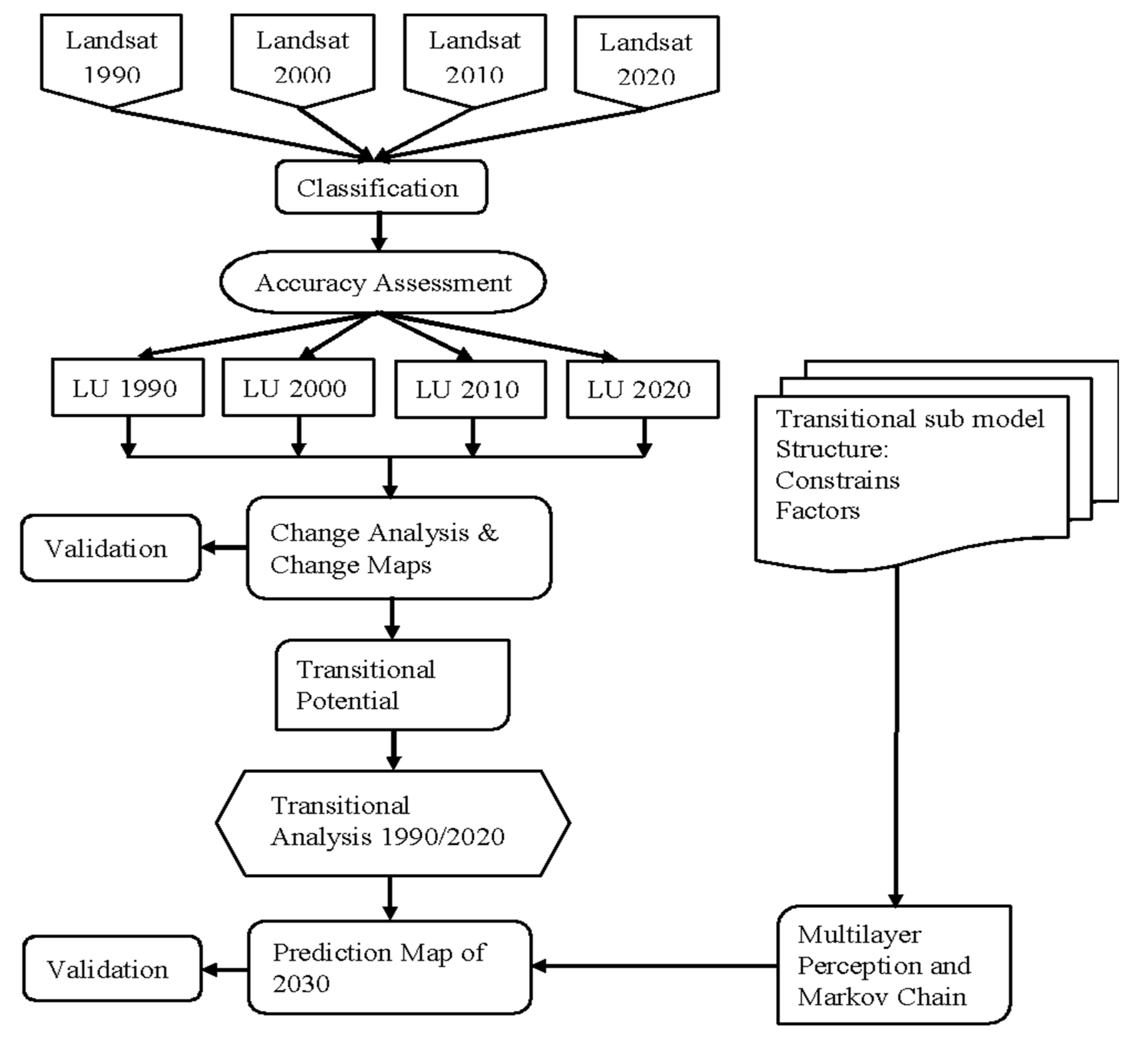
3. Materials and Methods

3.1. Data Sources

Satellite images covering the area of Batticaloa District were acquired from the USGS EarthExplorer website (https://earthexplorer.usgs.gov/, retrieved on 15 January 2021). Remote sensing images of Landsat TM (1990), Landsat ETM+ (2000, 2010), and Landsat OLI/TIRS (2020) were used with the spatial resolution of 30 m, georeferenced at the UTM projection zone 44 N, and resampled to 30 m with the nearest neighborhood algorithm (Table 1).

3.2. Land-Use Classification

In this study, the multi-temporal approach for extracting the information from satellite images was used to classify land-use by ERDAS Imagine software. Land utilization was classified into seven types, namely, agriculture, bare land, home garden, homestead, sandy, scrub, and wetland, using the maximum likelihood algorithm of the supervised classification. The supervised classification method is a grouping of pixels with common characteristics that is based on the machine learning algorithm of an image [32,33]. The pixels are determined into classes of a group by the machine-learning algorithm and the user can define which algorithm to use to achieve several output classes. The supervised classification is a composite image comprising a grouping of pixels [34]. However, when using the machine-learning technique, the user can observe that the grouping of the pixels with common characteristics relates to the actual features on the ground.

3.3. Land-Use (LU) Change

The Landsat images of the medium resolution were used to map the historic land-use change over 30 years in the BMC and then change images were used to simulate land-use for the next decade. The methodology employed to perform the whole process of the detection of land-use change and forecastingaredemonstrated in Figure 2. The ERDAS Imagine, (version 14), TerrSet (version 18.3), and ArcGIS (version 10.8) software were used for data analysis. Land-use images from 1990, 2000, 2010, and 2020 were used to detect the land-use changes for 1990–2000, 2000–2010, and 2010–2020.
The land change modeler is an integrated software platform developed by TerrSet for the analysis of the ecological sustainability of land-use and land-cover changes to support planning and policymaking [35]. This model tool is supported to extract information among the land-use classes of change scenarios [3,35,36]. The model provides three options.The first option is a rapid assessment of quantitative change by graphing gains and losses by land-use types. The second is net-change, which adds the previous land-cover areas for the gains and then subtracts the losses. The third option examines the contribution to changes experienced by single land-use [20]. This model also provides a better understanding of the functions of the land-use systems and the support needed for planning and policy-making [6,7].

3.4. Markov Chain LU Simulation

The land-use change images were used to predict the land-use in 2030 using the Markov chain simulation model. The Markov chain model uses several assumptions to estimate future land-use in a specific manner. Land-use change is a stochastic process, while it is denoted as the state of a chain [27,37]. This method quantifies the condition of status in the rapid change of land-use. Generally, this process can be performed based on a few conditional probabilities that can alter from one status to another in every time step [10]. This model determines land-use maps of the past, and prediction maps for the future, along with the specified dates [35]. The procedure accurately defines how much land would be expected to transition from the past date to the projected date, based on a prediction of the transition potentials forthcoming [5]. The Markov model produces transition matrices and a set of uncertain images by analyzing the temporal scale of land-use [26].
In this study, the future land-use changes are defined through a set of Markov chain transition probabilities matrices. Here the series of processes is stochastic that the value of the process at time t, Xt, depends only on its value at time t − 1, Xt−1, and not on the sequence of values Xt−2, Xt−3, …, X0 that the process passed through in arriving at Xt−1 [9]. The chain forms as follows:
P r   P r {   x t   =   j   |   x 0 = i 0 ,   x 1   = i 1 ,     .   x t 1   = i   } = P r { x t   = j   |   x t 1   = i   }
The   P r { x t   = j   |   x t 1   = i   } shows the one-step transitional probability, the process that provides the transition from state i to state j in one time period [37]. This study consists of a first-order standardized Markov chain.
In this event:
P r {   x t 1   = a i   } = P i j  
where Pij, the tabulate number, is shown from the experimental data from I to j [37]. The Markov chain improves by the time stationary, the land-use disseminations (t + 1) after tth transition period is s (t + 1) = s(t)P, where P is represented by the Markov transition matrix in the land-use types [19]. Once an adequately large time step ensues, the chain obtains a static state. Here, supply is controlled as S* = ( 0 ) P t ; however, it is independent of the initial distribution [9]. The maximum likelihood method is used to estimate for the best use of the constraint that j i   P i j   = 1 , and this yields [36]:
  P i j   = n i j   /   n i  
where   n i j   is the total number of observed cells from state i to j, and   n i   is the total number of cells transiting from state i [38]. Therefore, the study allows for testing a static and first-order Markov chain process.

4. Results

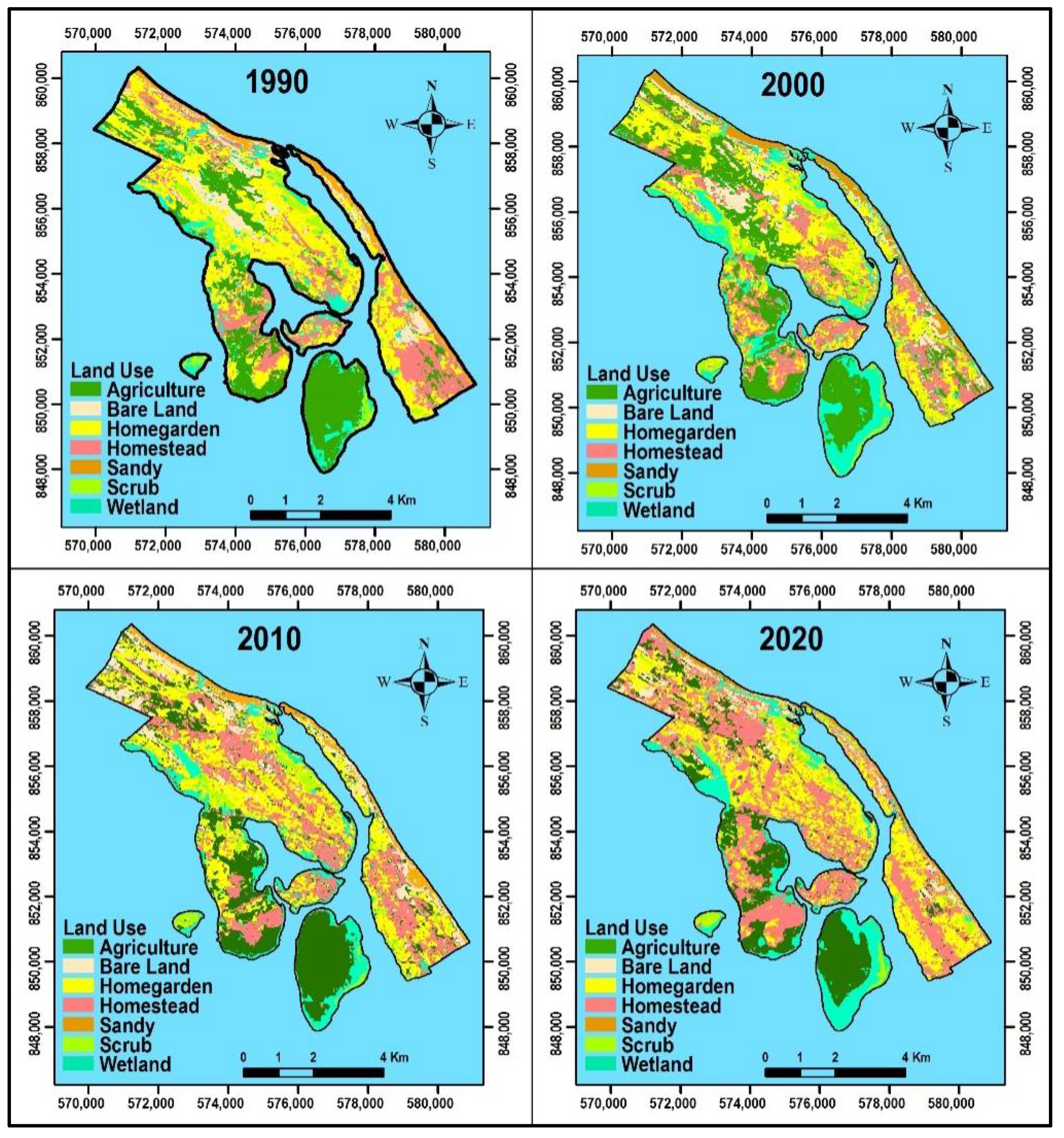
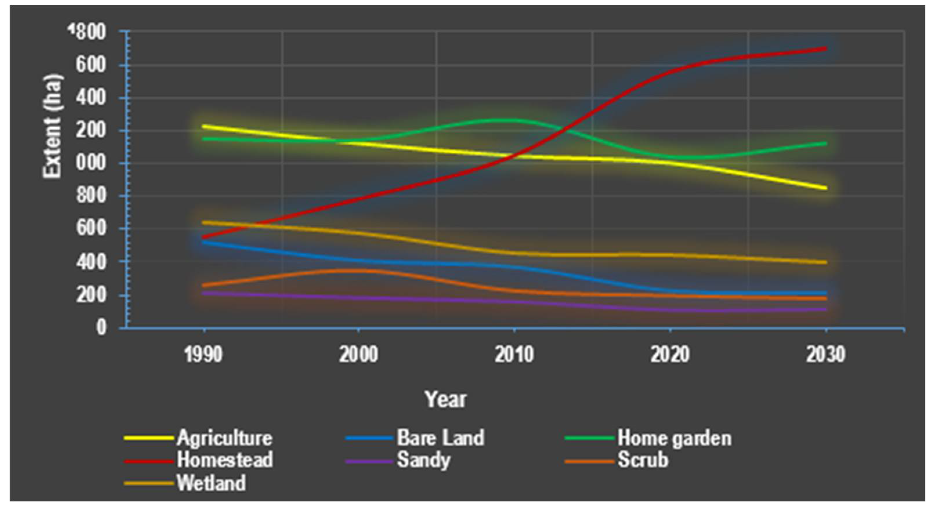
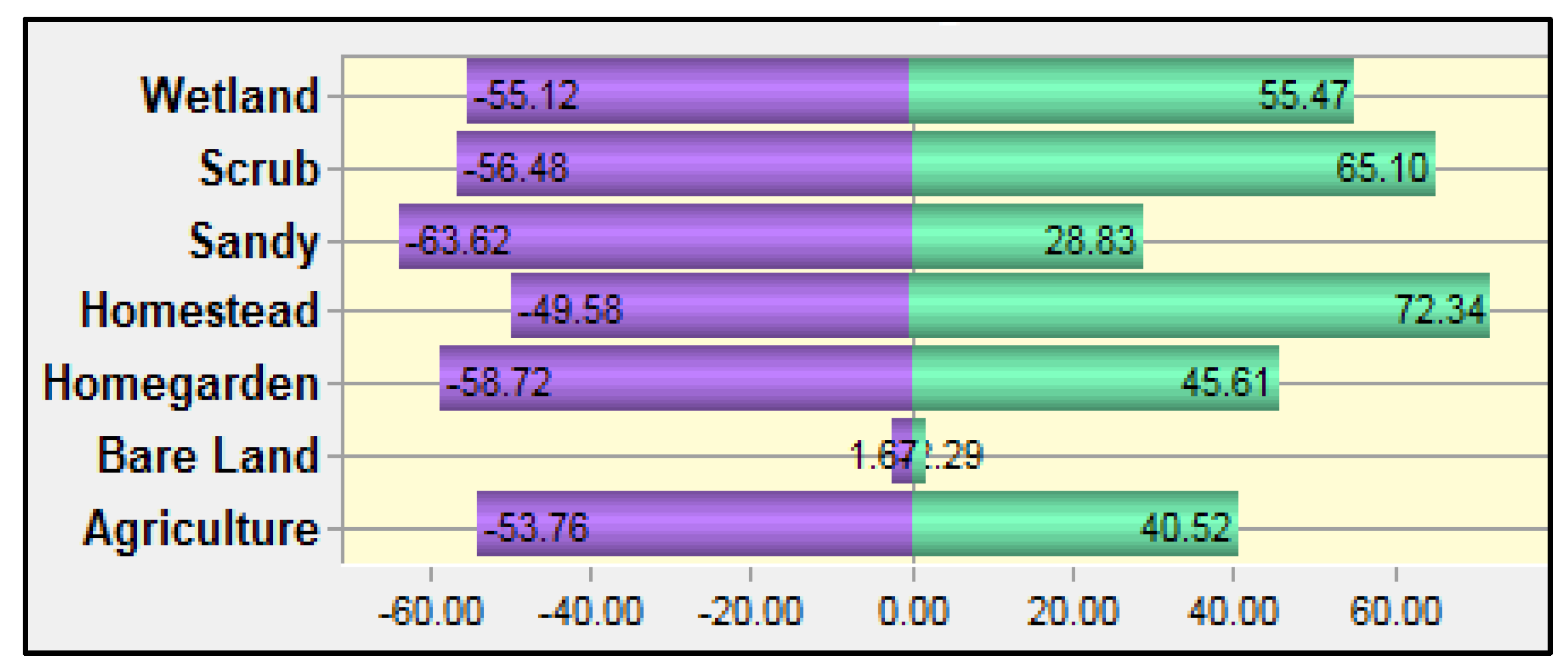
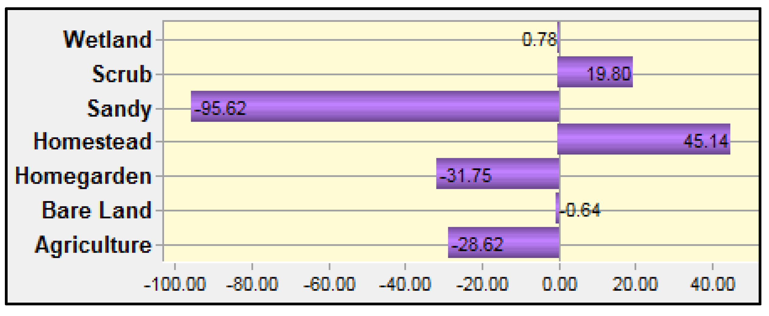
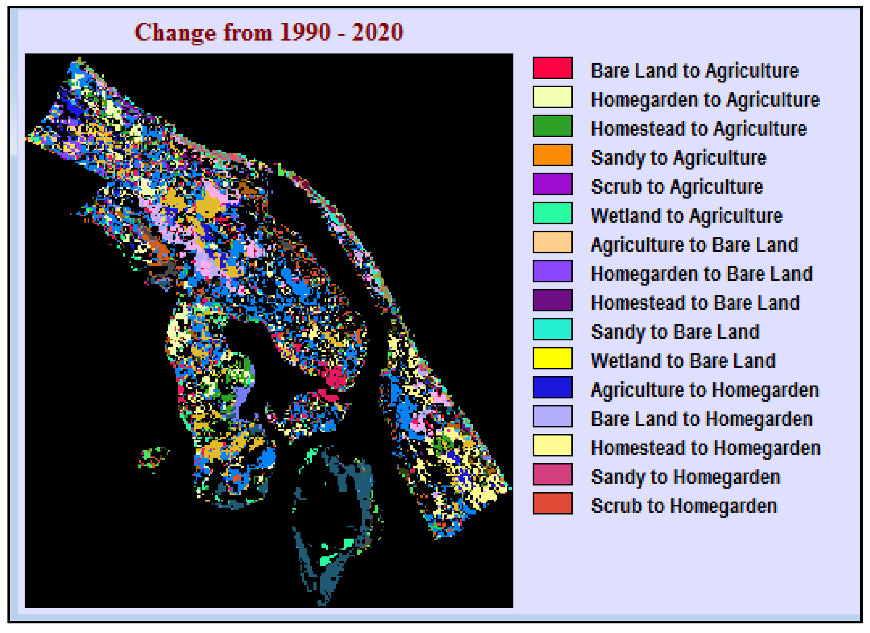
4.1. Land-Use Change from 1990 to 2020

The land-use classified images from 1990 to 2020 were compared in terms of the total area for each land-use type and was compared with reference data for accuracy assessment. A global positioning system (GPS) was used to field surveys as ground truth data to verify the classification accuracy. The accuracy assessment procedure is a very effective method to represent accuracy, with both errors of omission and commission, in land-use classification [39]. The overall accuracy of the images was 86.4% in 1990, 85.2% in 2000, 85.9% in 2010, and 87.1% in 2020 (Table 2). A high accuracy was obtained for sandy and bare land, while agriculture and wetland obtained a lower accuracy.
The temporal land-use change results show that the bare land had decreased to 2.5% from 1990 to 2000, to 3.3% from 1990 to 2010, and to 6.5% during the 1990 to 2020 periods. Similarly, agriculture had declined to 2.3%, 4.0%, and 5.0% for the 1990–2000, 1990–2010, and 1990–2020 periods, respectively (Table 3). Sandy and wetland also showed a declining trend over the 1990 to 2020 periods.
Homestead increased twice in each time step, i.e., 5.1% increased from 1990 to 2000, 10.9% increased from 1990 to 2010, and 22.0% increased during the 1990 to 2020 periods (Table 3).
Figure 3 presents the spatial distribution of land-use changes at a temporal scale. Land-use classes in the BMC can be categorized into two, namely, built-up (i.e., homestead and home garden), and non-built-up (agriculture, bare land, sandy, scrub, and wetland). In 1990, the built-up land area was about 1706.7 ha and it covered 37% of the total land area, while the built-up land area in 2020 was 2599.3 ha and it covered 56.9% of the total land area. Non-built-up land was limited to 1971.1 ha in 2020, which is just 43.1% of the total land area.

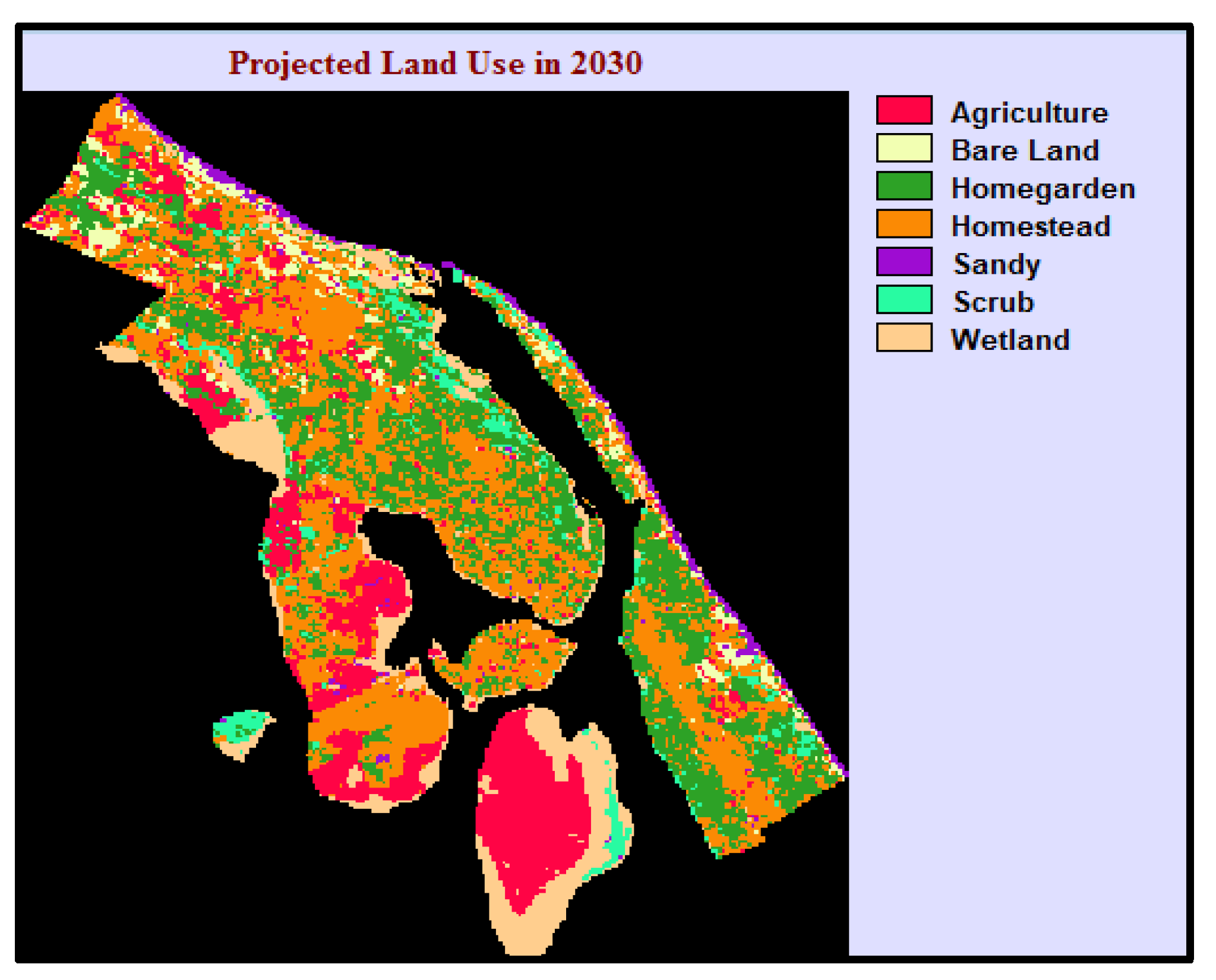
4.2. Land-Use Change in 2030

Based on the results, the trends forecast model of the BMC area is simulated as a percentage by the Markov chain. However, homesteads in the BMC had sharply increased from 12.7% in 2000 to 34.1% in 2020, and after 10 years, in the year 2030, land-use for homesteads might have increased to 37.3% (Figure 4).
It seems that the key factors for the increase in homesteadsare the rapid population increase, resettlements, increased service centers, and infrastructure developments. The simulated land-use changes from 1990 to 2030 in the BMC are shown in Figure 5.
Based on the LCM gain and loss analysis, the sandy area shows a higher loss of −63.6% while gaining 28.8%. Home garden, scrub, wetland, and agriculture illustrate more than 50% of the loss while a more than 50% gain of scrub and wetland is expressed. However, homestead shows 50% of the loss and a higher gain of 72.3% among the seven (07) land-use classes. The bare land illustrates the least loss and gains among the land-use types, accounting for a 1.7% loss, and a 1.3% gain, during 1990–2020 (Figure 6).
Based on the LCM net-change analysis, the sandy area has a higher negative change (−95.6%), followed by the home garden (−31.8%), agriculture (−28.6%), and bare land (−0.6%). While the homestead has a higher positive change to 45.1%, the scrub is 19.8% and wetland is 0.8% from 1990 to 2020 (Figure 7).
The certain land-use class is defined by the annual average rate of transitional probability values from one state to another. Table 4 depicts the transition probability of seven land-use classes, namely, agriculture, bare land, home garden, homestead, scrub, sandy, and wetland in the BMC. The transition probabilities from scrub to home garden, homestead, and agriculture are high. Bare land transition to homestead and agriculture is also high. Wetland is the most unchanged land-use based on the transition probabilities.
As a result, the land-use class will change into another land-use type through the transition probability matrix in the future [19]. From Equation (3), in 1990, the certain land-use type converted into the same land-use, which was represented in 2000. However, homestead land-use rarely transfers to other land-use classes in the study. Here, the transition probabilities observed that homestead state to other states as nearly ‘zero’ values without home garden land-use because land-use of the home garden was uncertain due to the civil war in the Eastern Province of Sri Lanka.
On the basis of the results, the land-uses of the home garden–homestead, agriculture–homestead, agriculture–wetland, and bare land–homestead have shown higher-level changes in more than 200 ha. Similarly, in the changes from 100 to 200 ha, the land classes show as agriculture–home garden, bare land–home garden, wetland–agriculture, scrub–home garden, and home garden–agriculture. All other land-use has been transformed to less than 100 ha (Figure 8).

5. Discussion

This study provides information on the spatiotemporal land-use changes that occurred during 1990–2020 in the municipal council limits of Batticaloa and combines the empirical land-use model to simulate the land-use change in 2030. We used theland change modeler as a decision support land planning tool [6,7] to evaluate historical land-use changes (from 1990 to 2020) in the BMC, and the Markov chain stochastic simulation model (for example, [7,8,10,27,29,38,40]) to predict land-uses in 2030. Change detection is important for determining which land-use is changing, and how it is changing, for sustainable land-use planning [40,41,42,43]. The future forecast map of 2030 is useful for developing suitability modeling for homesteads, which were growing exponentially from 2010 to 2020.The land-uses in the BMC have changed because of human-induced activities, such as illegal mining, plantations, sprawling development, encroachment, and natural events, such as storm surges and floods [31,41,42]. An unpredictable sociopolitical system has caused a rapid change in land-use and land-cover in Batticaloa over the past twenty years [43].
Most of our land-use class accuracy (both producer’s and user’s accuracy) is greater than 80%, which is considered a moderate accuracy for classification [7,41,44]. In remote sensing data, the minimum level of accuracy assessment should be determined as at least 85% in land-use types [45]. The accuracy of sandy land-use is comparatively higher (≥94% ≤100%) than other land-uses that are confined to a narrow strip of shoreline/sandbelt (Table 2, Figure 4). The sandy beaches in this area are unique and are characterized by bays and headlands, straight sandy shoreline/beaches, deltas/saline flats, and sparse vegetation [41]. Bare land has limited resources for supporting life and can be easily identified while training the data and, therefore, the accuracy of bare land is noticeably high (≥96% ≤100%).
There was an increase in homesteads between 2010 and 2020 (Figure 5) as a consequence of the civil war ending in 2009 and the migration of people to an area with a peaceful environment and infrastructure facilities. Agriculture is declining over time (Figure 4), and this could be an impact of the tsunami effect in 2004 where the saltwater intrusion onto agricultural lands resulted in infertile or bare lands. Home garden acreage was just over the agriculture lands in the year 2000 and onward and seems to be increasing with the increase in homesteads. Similarly, Partheepan et al. [43] found that the cultivated areasin Batticaloa have increased by 41.9% from 2000 to 2005 because of the peace process prevailing in the country at that time.
The Markov chain model has coupled with geospatial technology in the descriptive capability of prediction. This spatiotemporal model provides, not only a quantitative description of the changes in earlier times, but also the path and level of change in the future. In this study, based on experimental results and empirical analysis, limitations are present. However, four images were used to analyze the land-use change and the images were acquired on different dates (Figure 3). In the Markov chain model, the transition probability is expected to be uniform with the images. Therefore, it is challenging to accommodate variables by random influence, such as the climatic condition and human influence [46]. However, it can be resolved by combining temporal, high-accuracy, and same-dated images for decision-making in long-term forecasts.

6. Conclusions

The aim of this study is based on the geospatial technology analysis of land-use change and a modeling of future land-use in the BMC. The Markov chain model simulates changes in land-use using multi-dated Landsat images from 1990–2020. The results show that the areas of homestead in the BMC increased by 12.7% to 34.1% from 1990 to 2020. During this period, land-use classes of agriculture, wetland, home garden, sandy, and scrub decreased to 5.0%, 4.3%, 2.5%, 2.3%, and 1.4%, respectively. Our results clearly show that the built-up area has gradually increased from 1990 (37.3%) to 2020 (56.8%), while the non-built-up area has declined from 62.7% to 43.1% for the period. The land-use trends were simulated for the forthcoming decade through the use of the Markov model. The results indicate that homestead and built-up areas will have increased by 37.3% and 61.8% in the year 2030, respectively. This result shows that the natural equilibrium of the BMC is threatened by the population pressure of the last 30 years. The historical and forecasting land-use model is important to make better land-use planning decisionsin the BMC for mitigating climatic (e.g.,a tsunami) and/or anthropogenic impacts.

Author Contributions

Conceptualization, I.L.M.Z.; methodology, I.L.M.Z.; formal analysis, I.L.M.Z.; writing—original draft preparation, I.L.M.Z.; writing—review and editing, S.T.; writing—review and editing, R.P.S.; writing—review and editing, J.H., B.M.; writing—review and editing, A.L.I. All authors have read and agreed to the published version of the manuscript.

Funding

This research received no external funding.

Institutional Review Board Statement

Not applicable.

Informed Consent Statement

Not applicable.

Data Availability Statement

Not applicable.

Conflicts of Interest

The authors declare no conflict of interest.

References

  1. FAO. Planning for Sustainable Use of Land Resources; FAO Land and Water Bulletin: Rome, Italy, 1995; 53p. [Google Scholar]
  2. Hasan, S.; Shi, W.; Zhu, X.; Abbas, S.; Ahmed Khan, H.U. Future simulation of land use changes in rapidly urbanizing South China based on land change modeler and remote sensing data. Sustainability 2020, 12, 4350. [Google Scholar] [CrossRef]
  3. Ahmed, B.; Ahmed, R. Modeling Urban Land Cover Growth Dynamics Using Multi-Temporal Satellite Images: A Case Study of Dhaka, Bangladesh. ISPRS Int. J. Geoinf. 2012, 1, 3–31. [Google Scholar] [CrossRef] [Green Version]
  4. Aithal, B.H.; Vinay, S.; Ramachandra, T.V. Prediction of Landuse Dynamics in the Rapidly Urbanising Landscape using Land Change Modeller. In Proceedings of the Advances in Computer Science, Delhi, India, 13–14 December 2013. [Google Scholar]
  5. Wang, J.; Maduako, I.N. Spatio-temporal urban growth dynamics of Lagos Metropolitan Region of Nigeria based on Hybrid methods for LULC modeling and prediction. Eur. J. Remote Sens. 2018, 51, 251–265. [Google Scholar] [CrossRef] [Green Version]
  6. Kumar, K.S.; Bhaskar, P.U.; Padmakumari, K. Application of Land Change Modeler for Prediction of Future Land Use Land Cover a Case Study of Vijayawada City. Int. J. Adv. Technol. Eng. Sci. 2015, 3, 773–783. [Google Scholar]
  7. Kumar, S.; Radhakrishnan, N.; Mathew, S. Land use change modeling using a Markov model and remote sensing. Geomat. Nat. Hazards Risk 2014, 5, 145–156. [Google Scholar] [CrossRef]
  8. Madurapperuma, B.; Rozario, P.; Oduor, P.; Kotchman, L. Land-use and land-cover change detection in Pipestem Creek watershed, North Dakota. Int. J. Geomat. Geosci. 2015, 5, 416–426. [Google Scholar]
  9. Adepoju, M.O.; Millington, A.C.; Tansey, K.T. Land Use/Land Cover Change Detection in Metropolitan Lagos (Nigeria): 1984–2000. AASPRS 2006 Annu. Conf. Reno Nev. 2006, 1–5. [Google Scholar]
  10. Mondal, M.S.; Sharma, N.; Garg, P.K.; Kappas, M. Statistical independence test and validation of CA Markov land use land cover (LULC) prediction results. Egypt. J. Remote Sens. Space Sci. 2016, 19, 259–272. [Google Scholar] [CrossRef] [Green Version]
  11. Lal, A.M.; Anouncia, M.S. Semi-supervised change detection approach combining sparse fusion and constrained k means for multi-temporal remote sensing images. Egypt. J. Remote Sens. Space Sci. 2015, 18, 279–288. [Google Scholar] [CrossRef] [Green Version]
  12. Chilar, J. Land Cover Mappings of Large Areas from Satellite: Status and Research Priorities. Remote Sens. Environ. 2003, 21, 1090–1114. [Google Scholar]
  13. Kachhwala, T.S. Temporal Monitoring of Forest Land for Change and Forest cover Mapping through Satellite Remote Sensing. Proc. 6th Asian Conf. Remote Sens. Natl. Remote Sens. Agency Hyderabad 1985, 1985, 77–83. [Google Scholar]
  14. Lo, C.P.; Choi, J. A Hybrid Approach to Urban Land Use/Cover Mapping using Landsat 7 Enhanced Thematic Mapper Plus (ETM+) images. Int. J. Remote Sens. 2004, 25, 2687–2700. [Google Scholar] [CrossRef]
  15. Islam, K.; Jashimuddin, M.; Nath, B.; Nath, T.K. Land use classification and change detection by using multi-temporal remotely sensed imagery: The case of chunati wildlife sanctuary, Bangladesh. Egypt. J. Remote Sens. Space Sci. 2017, in press. [Google Scholar] [CrossRef]
  16. Brondizio, E.S.; Moran, E.F.; Wu, Y. Land Use Change in the Amazon Estuary: Patterns of Caboclo Settlement and Landscape Management. Hum. Ecol. 1994, 22, 249–278. [Google Scholar] [CrossRef]
  17. Uduporuwa, R.J.M. Spatial and Temporal Dynamics of Land Use/Land Cover in Kandy City, Sri Lanka: An Analytical Investigation with Geospatial Techniques. Am. Sci. Res. J. Eng. Technol. Sci. 2020, 69, 149–166. [Google Scholar]
  18. Department of Social and Economic Affairs, United Nation. 2018 Revision of World Urbanization Prospects. 2018. Available online: https://www.un.org/development/desa/publications/2018-revision-of-world-urbanization-prospects.html (accessed on 5 June 2021).
  19. Wu, Q.; Li, H.Q.; Wang, R.S. Monitoring and predicting land-use change in Beijing using remote sensing and GIS. Landsc. Urban Plan. 2006, 78, 322–333. [Google Scholar] [CrossRef]
  20. Verburg, P.H.; Schot, P.P.; Dijst, M.J.; Veldkamp, A. Land use change modelling: Current practice and research priorities. Geo. J. 2004, 61, 309–324. [Google Scholar] [CrossRef]
  21. Eastman, J.R.; Toledano, J. A Short Presentation of the Land Change Modeler (LCM). In Geomatic Approaches for Modeling Land Change Scenarios; CamachoOlmedo, M., Paegelow, M., Mas, J.F., Escobar, F., Eds.; Geomatic Approaches for Modeling Land Change Scenarios. Lecture Notes in Geoinformation and Cartography; Springer: Cham, Switzerland, 2018. [Google Scholar]
  22. Han, H.; Yang, C.; Song, J. Scenario Simulation and the Prediction of Land Use and Land Cover Change in Beijing, China. Sustainability 2015, 7, 4260–4279. [Google Scholar] [CrossRef] [Green Version]
  23. Nourqolipour, R.; Mohamed Shariff, A.R.B.; Balasundram, S.K.; Ahmad, N.B.; Sood, A.M.; Buyong, T.; Amiri, F. A GIS-based model to analyze the spatial and temporal development of oil palm land use in Kuala Langat district, Malaysia. Environ. Earth Sci. 2015, 73, 1687–1700. [Google Scholar] [CrossRef] [Green Version]
  24. Mas, J.F.; Kolb, M.; Paegelow, M.; Olmedo, M.C.; Houet, T. Modelling Land use/cover changes: A comparison of four software packages. Environ. Model. Softw. 2014, 51, 94–111. [Google Scholar] [CrossRef] [Green Version]
  25. Megahed, Y.; Cabral, P.; Silva, J.; Caetano, M. Land Cover Mapping Analysis and Urban Growth Modelling Using Remote Sensing Techniques in Greater Cairo Region-Egypt. ISPRS Int. J. Geo-Inf. 2015, 4, 1750–1769. [Google Scholar] [CrossRef] [Green Version]
  26. Mishra, V.N.; Rai, P.K.; Mohan, K. Prediction of land use changes based on land change modeler (LCM) using remote sensing: A case study of Muzaffarpur (Bihar), India. J. Geogr. Inst. Cvijic. 2014, 64, 111–127. [Google Scholar] [CrossRef]
  27. Ozturk, D. Urban Growth Simulation of Atakum (Samsun, Turkey) Using Cellular Automata-Markov Chain and Multi-Layer Perceptron-Markov Chain Models. Remote Sens. 2015, 7, 5918–5950. [Google Scholar] [CrossRef] [Green Version]
  28. Hone-Jay, C.; Yu-Pin, L.; Chen-Fa, W. Forecasting Space-Time Land Use Change in the Paochiao Watershed of Taiwan Using Demand Estimation and Empirical Simulation Approaches; Taniar, D., Gervasi, O., Murgante, B., Pardede, E., Apduhan, B.O., Eds.; Springer: Berlin/Heidelberg, Germany, 2010; pp. 116–130. [Google Scholar]
  29. Shafizadeh, H.M.; Helbich, M. Spatiotemporal urbanization processes in the megacity of Mumbai, India: A Markov chains-cellular automata urban growth model. Appl. Geogr. 2013, 40, 140–149. [Google Scholar] [CrossRef]
  30. UDA. Approval of Development Plan for Batticaloa Municipal Council, Ministry of Defense and Urban Development, Colombo. 2013. Available online: https://www.uda.gov.lk/development-plans-reports.html?plan=2 (accessed on 9 October 2013).
  31. Mathanraj, S.; Ratnayake, R.M.K.; Rajendram, K. A GIS-Based Analysis of Temporal Changes of Land Use Pattern in Batticaloa MC, Sri Lanka from 1980 to 2018. World Sci. News 2018, 137, 210–228. [Google Scholar]
  32. Coskun, G.H.; Alganci, U.; Usta, G. Analysis of land-use change and urbanization in the Kucukcekmece water basin (Istanbul, Turkey) with temporal satellite data using remote sensing and GIS. Sensors 2008, 8, 7213–7223. [Google Scholar] [CrossRef] [PubMed] [Green Version]
  33. Lillesand, T.M.; Kiefer, R.W. Remote Sensing and Image Interpretation; John Wiley and Sons: New York, NY, USA, 2003. [Google Scholar]
  34. Madurapperuma, B.D.; Dellysse, J.E.; Iyoob, A.L.; Zahir, I.L.M. Mapping coastal fringe community variability of Pottuvil using high-resolution kite aerial photography. In Proceedings of the Peradeniya University International Research Sessions, Kandy, Sri Lanka, 21–24 November 2017. [Google Scholar]
  35. Clark Labs. The Land Change Modeler for Ecological Sustainability; IDRISI Focus Paper; Clark University: Worcester, MA, USA, 2009; Available online: http://www.clarklabs.org/applications/upload/Land-Change-Modeler-IDRISI-Focus-Paper-pdf (accessed on 22 September 2021).
  36. Costanza, R.; Ruth, M. Using Dynamic Modeling to Scope Environmental Problems and Build Consensus. Environ. Manag. 1998, 22, 183–195. [Google Scholar] [CrossRef] [PubMed]
  37. Weng, Q. Land use change analysis in the Zhujiang Delta of China using satellite remote sensing, GIS and stochastic modeling. J. Environ. Manag. 2002, 64, 273–284. [Google Scholar] [CrossRef] [Green Version]
  38. Billingsley, P. Statistical methods in Markov chains. Ann. Math. Stat. 1961, 32, 12–40. [Google Scholar] [CrossRef]
  39. Congalton, R.G. A review of assessing the accuracy of classification of remotely sensed data. Remote Sens. Environ. 1991, 37, 35–46. [Google Scholar] [CrossRef]
  40. Madurapperuma, B.; Oduor, P.; Kotchman, L. Detecting Land-Cover Change using Stochastic Simulation Models and Multivariate Analysis of Multi-Temporal Landsat Data for Cass County, North Dakota. Environ. Nat. Resour. Res. 2013, 3, 78. [Google Scholar] [CrossRef] [Green Version]
  41. Mathiventhan, T.; Jayasingam, T. Geomorphological changes along the East Coast of Sri Lanka. Intern. J. Res. Stud. Biosci. 2018, 6, 6–12. [Google Scholar]
  42. Mathanraj, S.; Rusli, N.; Ling, G.H.T. Applicability of the CA-Markov Model in Land-use/Land cover Change Prediction for Urban Sprawling in Batticaloa Municipal Council, Sri Lanka. In IOP Conference Series: Earth and Environmental Science; IOP Publishing: Bristol, UK, 2021; Volume 620, p. 012015. [Google Scholar]
  43. Partheepan, K.; Manobavan, M.; Dayawansa, N. Assessment of land-use changes in the Batticaloa district (2000–2003/2005) for the preparation of a (spatial) zonation plan to aid in decision making for development. JSc. East. Univ. Sri Lanka 2008, 5, 19–31. [Google Scholar]
  44. Jensen, J.R. Introductory Digital Image Processing: A Remote Sensing Perspective, 3rd ed.; Prentice-Hall, Inc.: Hoboken, NJ, USA, 2005. [Google Scholar]
  45. Anderson, J.R.; Hardy, E.E.; Roach, J.T.; Witmer, R.E. A Land Use and Land Cover Classification System for Use with Remote Sensor Data; Government Printing Office: Washington, DC, USA, 1976. [Google Scholar]
  46. Mahanama, P.K.S.; Abenayake, C.; Jayasinghe, A. Climate Change Vulnerability Assessment. Available online: https://www.fukuoka.unhabitat.org/programmes/ccci/pdf/SRL5_Vulnerability_Assessment_Batticaloa.pdf (accessed on 22 September 2021).
Figure 1. Study area showing 48 GramaNiladhari Districts (GNDs) in Batticaloa District.
Geographies 01 00010 g001
Figure 2. Flowchart of land-use change detection in the BMC using the Land Change Modeler.
Geographies 01 00010 g002
Figure 3. Land-use changes in 1990, 2000, 2010, and 2020 in the BMC.
Geographies 01 00010 g003
Figure 4. Prediction of land-use for 2030 in the BMC.
Geographies 01 00010 g004
Figure 5. Simulated land use change from 1990 to 2030.
Geographies 01 00010 g005
Figure 6. Percentage of gain and loss of land use from 1990 to 2020.
Geographies 01 00010 g006
Figure 7. Percentage of the net-change of land use from 1990 to 2020.
Geographies 01 00010 g007
Figure 8. Land-use change in the BMC between 1990 and 2020.
Geographies 01 00010 g008
Table 1. Satellite images sensor information.
Sensor NameAcquisition DateRow/PathSpatial Resolution
Landsat 5 TM12 September 199055/14030 m
Landsat 7 ETM+7 May 200055/14030 m
Landsat 7 TM1 April 201055/14030 m
Landsat 8 OLI/TIRS27 September 202055/14030 m, Pan.-15 m
Table 2. Accuracy assessment of land-use classified images.
Categories1990200020102020
PA (%)UA (%)PA (%)UA (%)PA (%)UA (%)PA (%)UA (%)
Agriculture69.781.371.985.178.689.477.891
Bare Land98.210096.498.797.910098.299.8
Homegarden8891.486.998.389.297.391.697.6
Homestead87.171.781.979.289.785.48881.1
Sandy10010099.110093.799.6100100
Scrub97.698.889.288.691.389.591.790.1
Wetland76.269.878.584.477.889.182.384.7
Overall Accuracy86.485.285.987.1
Kappa Coefficient82.381.780.283.6
Table 3. The land-use types in the BMC from 1990–2020, and a comparison of the extent of land-use in 2030, simulated by a Markov Chain.
Land-Use Types19902000201020202030ChangeChangeChange
Extent (ha)Extent (ha)Extent (ha)Extent (ha)Extent (ha)(1990–2000)(1990–2010)(1990–2020)
Agriculture12311125.71046.91003.2846.9−2.3−4−5
Bare Land525.4413.21372.9227.2214.4−2.5−3.3−6.5
Home garden11521142.81266.41039.71123.6−0.22.5−2.5
Homestead554.7786.31050.91559.61702.95.110.922
Sandy210.9181.7157.5105110.1−0.6−1.2−2.3
Scrub259.7348.5224.7195.3177.51.9−0.8−1.4
Wetland636.7572.3451.2440.4395.2−1.4−4.1−4.3
Built-up1706.71929.12317.32599.32826.54.913.319.5
−37.3%−42.2%−50.7%−56.8%−61.8%
Non-built-up2863.72641.42253.21971.11744.1−4.9−13.3−19.5
−62.7%−57.8%−49.3%−43.1%−38.1%
Table 4. Probability transition matrix of land-use classes in 1990 and 2020.
YearProbability of Changing of Land-Use Classes 2020
1990Land-Use ClassesAgricultureBare LandHome GardenHomesteadSandyScrubWetland
Agriculture0.60620.01340.01540.14890.00110.04360.1715
Bare Land0.23270.27810.08710.39610.00170.00430
Home garden0.02060.00610.44080.4090.00510.10330.015
Homestead0.005400.39420.59680.003100.0005
Sandy00.334100.150.4120.04620.0577
Scrub0.25520.1080.31390.281300.04160
Wetland0.032700.060100.01270.07240.8222
Publisher’s Note: MDPI stays neutral with regard to jurisdictional claims in published maps and institutional affiliations.

