
The Spatiotemporal Characteristics and Dynamic Changes of Tidal Flats in Florida from 1984 to 2020


Department of Geosciences, Florida Atlantic University, Boca Raton, FL 33431, USA
*
Author to whom correspondence should be addressed.
Geographies 2021, 1(3), 292-314; https://0-doi-org.brum.beds.ac.uk/10.3390/geographies1030016
Submission received: 31 October 2021
/
Revised: 13 November 2021
/
Accepted: 17 November 2021
/
Published: 19 November 2021
(This article belongs to the Special Issue Early Career Scientists’ (ECS) Contributions to Geographies)
Abstract
:Tidal flats are playing a critical role in the coastal environment, which mainly rely on satellite images to map the distribution on large spatiotemporal scales. Much effort has been made to monitor and analyze the spatiotemporal dynamics of tidal flats in order to provide worthwhile references for scientists and lawmakers. Instead of considering the dynamics of tidal flats only, this study implemented a series of comprehensive analyses on the tidal flats along the coast of Florida during the period 1984–2020. First, the analyses on the pixel level examined the spatiotemporal characteristics of tidal flat dynamics and the interactions with lands and permanent water. Second, the contiguous pixels of tidal flats were assembled as objects, and two geometric attributes were calculated and used to track the temporal patterns of tidal flat dynamics on this level. Finally, the Mann–Kendall test and Sen’s slope estimator were applied to identify and quantify the significant trends of tidal flat dynamics on the two levels. The results highlighted the differences in tidal flat distributions and dynamics between the Gulf Coast and Atlantic Coast, which further verified effective GIS representations and analyses that could be applied to other coastal studies.
1. Introduction
Owing to the sufficient supply of the fine-grained sediments and the hydrodynamic forces dominated by tides, a unique type of environment is constituted along the coast, which is also known as tidal flats [1]. This area is characterized by the intensified interactions between land and sea, which makes it the natural transitions between ocean and terrestrial ecosystems and consequently acts a critical role in the biodiversity on Earth [2,3]. Located at the forefront of the ocean, tidal flats also play an irreplaceable role in protecting the lands from margin erosions and flooding due to tidal currents, waves, tsunamis, and hurricanes [4,5]. Moreover, the coastal residents have gained considerable economic profits from tidal flats, including but not limited to fishery [6] and aquaculture [7]. While tidal flats have tremendously contributed to the coastal environments and communities, they are under increasing pressure from intensive human activities. For example, tidal flats have become a land source for urban expansions [8,9], and the urban wastes have further deteriorated the environmental crisis of tidal flats [10]. As the counterforce from damaged environment, the natural hazards could risk the safety of coastal communities and consequently the densely populated communities are even more vulnerable [11]. On a global scale, tidal flats declined by 16.02% during 1984 to 2016 [12], which is a warning sign and urgently calls for the awareness and protections. To provide a worthwhile reference for scientists and lawmakers, a preparatory task is to monitor the dynamic changes of tidal flats.
To date, numerous frameworks have been proposed to map the distributions of tidal flats, which provide a solid foundation to monitor the tidal flat dynamics on large spatiotemporal scales. For example, the annual distributions of tidal flats in China from 1986 to 2016 were mapped according to the frequencies of water and vegetation [2]. Likewise, a more recent study [13] used Otsu’s thresholding [14] to optimize the segmentation of satellite imageries and mapped the distribution of tidal flats in China with an overall accuracy of 95%. On the other hand, the machine learning algorithms, such as Random Forests (RF), have been verified effective to automate the classification. Meanwhile, the high-performance cloud computing platforms, such as the Google Earth Engine (GEE), have demonstrated great potentials in the processing of big geospatial data. Consequently, several RF-based models have been proposed and realized through GEE, which greatly saved the labor and accelerated the progress of mapping. For example, a total of 48 statistical values were defined in the RF classifier proposed by Zhang et al. (2019) [15], and the distributions of tidal flats in China circa 2015 were mapped. Moreover, the RF-based framework given by Murray et al. (2019) [12] mapped the distribution of tidal flats throughout the whole world from 1984 to 2016, which unprecedentedly draw a picture to visualize and analyze the tidal flat dynamics on a large spatiotemporal scale. Acknowledging the limitations of existing frameworks, a new RF classifier was proposed with respect to the local conditions and used to produce the annual tidal flat maps throughout the conterminous United States (US) from 1984 to 2020 [16], which was also selected by this study to derive the fundamental tidal flat data for dynamic analyses.
Aside from the dynamic analyses on tidal flats, an in-depth consideration is to explore the spatiotemporal characteristics of the interactions between tidal flats and other land cover types. For example, a case study of Zhuhai City, China [17] assessed the gains and losses of tidal flats and other ecological lands between 1991 and 2018, during which the urban area had rapidly expanded. In addition, a model of ecological land change process was proposed with respect to multiple geographical factors, which was used to predict the land cover conversions in the future. Another case study of Zhoushan, China [18] generated the land cover maps in 1995 and 2011, in which the lands were classified into five categories, including woodland, farmland, water body, urban land, and tidal flats. Then, the maps in the two years were overlapped and compared, which finds the spatial distributions and the land sources of newly urbanized areas. A follow-up study [8] utilized the full time series of Landsat imageries archived in GEE to produce the monthly maps of coastlines and tidal flats from 1985 to 2017, which tremendously extended data availability on assessing the spatiotemporal patterns of land cover changes. Based on the monthly maps, that study explored the six types of interactions between lands, waterbodies, and tidal flats, and the identified spatiotemporal patterns were summarized and visualized. Again, in Zhoushan, China, a more recent study [9] inspected the urban expansions between 1986 and 2017 and mapped the newly urbanized areas with respect to the land source and the conversion year. The study found that 14 km2 tidal flats were urbanized during the 31 years, which corresponds to 4% of the total newly urbanized area.
Nevertheless, these pixel-wise analyses have critical limitations which raise concerns of the application in further assessments. Taking Cao et al. (2020) [8] for example, one pixel could have experienced multiple times of land cover conversions during these years, and accordingly the results were summarized by the most recent change on each pixel. Indeed, the mapping product is highly influenced by the spectral composition of each individual pixel on satellite imageries, and therefore cannot avoid misclassifications due to bad observations and random errors [19]. On the other hand, it ignores the relationships between different pixels, and the spatiotemporal information of every individual pixel is trivial and isolated [20]. More importantly, the study subjects exist in the real world, and the spatiotemporal change patterns are driven by natural or anthropogenic factors. Therefore, it is necessary to explore the backgrounds, rather than treat the geographical phenomena as abstract terms on the raster imageries. As Couclelis (1992) [21] claimed, the new generation of Geographic Information Science (GIS) should “be open to the notion of spatial representations that may not be mappable, and to GIS that do not work primarily through map-like displays”. The discussion of field modeling by Goodchild et al. (2007) [22] gives a solution to overcome the above limitations. Specifically, it regards the pixels as geo-atoms, and the geo-atoms can further aggregate as geo-fields. Accordingly, the object level analyses, which assemble the contiguous pixels as single patches, have been applied to multiple domains [23,24,25] and verified as an effective way to examine the spatiotemporal characteristics of dynamic geographic phenomena. Specifically speaking, the states of an individual object are characterized by the shapes at specific moments, which can be quantified by a variety of geometry attributes such as area, perimeter, roundness, and so on.
At this point, the priority is to monitor the dynamics of tidal flats in those large littoral countries, through which we can observe the spatiotemporal characteristics and summarize the trends on large scales. The US has the eighth longest coastline throughout the world [26] and therefore is a worthwhile region to investigate, but the relative research in this country progressed at a slow pace. Specifically speaking, we noticed the works in Chesapeake and Delaware Bays [27], Nisqually River Delta [28], Waccasassa Bay [29], and Eastern Gulf Coast [30], which glanced through the distributions of tidal flats in some selected places of the US. However, these studies focus on the small areas and therefore none of them could provide an assessment on a large scale to better understand the general change patterns. Moreover, these studies concentrate on tidal flat mapping, which is a fundamental work and still requires substantial analysis and in-depth exploration. Prior to analyzing the dynamics throughout the entire country, it is necessary to verify the effectiveness of the proposed method in a single state, and Florida was selected in this study. Florida has the second longest coast among the fifty states [31], which is sufficient to implement a comprehensive analysis on a large scale. Although Alaska has a longer coastline, the mapping framework aiming at Arctic region is yet to come [12] and therefore that state was not selected as the study area.
As stated above, we realized the practical challenges in tidal flat monitoring, as well as the gaps to fill, and accordingly determined the objectives of this study. Specifically speaking, this study applies innovative GIS representations and analyses to identify and characterize the spatiotemporal patterns of tidal flat dynamics on the two levels (pixel and object). It does not focus on the tidal flats only but also explores the interactions with the lands and permanent water. Meanwhile, we identified and quantified the evolutionary trends on the two levels, which provides an in-depth inspection for the temporal change patterns of tidal flats along the coast of Florida from 1984 to 2020. The implementation details were elucidated in Section 2. The results were illustrated in Section 3, which were further analyzed and discussed with respect to the geographical backgrounds. Finally, we summarized the significance of this study and discussed the direction of the future work (Section 4).
2. Materials and Methods
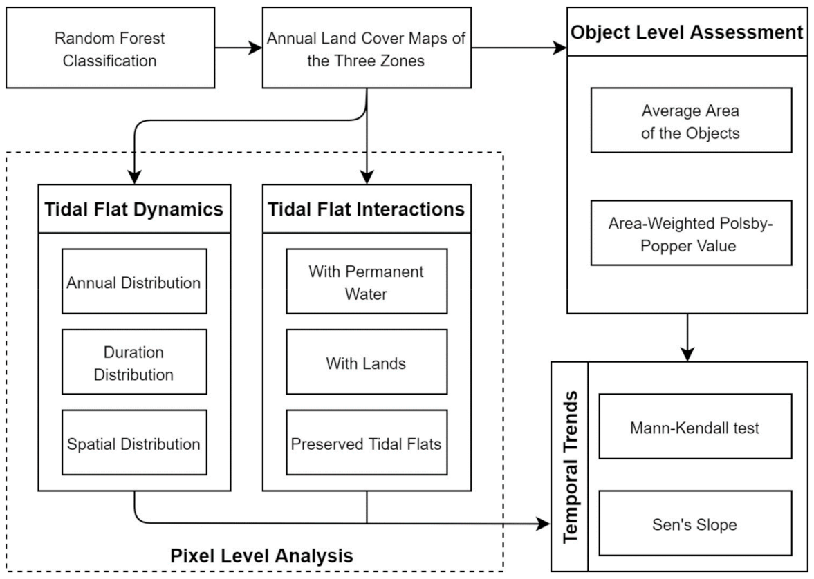
A framework was proposed to analyze the spatiotemporal characteristics and dynamic changes of tidal flats within the study area from 1984 to 2020 (Figure 1). As the preparatory task, the study area was divided into three zones (Section 2.1), and a RF model was used to generate the annual land cover maps during these 37 years for each zone (Section 2.2). The classified maps were analyzed on the pixel level (Section 2.3) and object level (Section 2.4), and the Mann–Kendall test and Sen’s slope estimator were utilized to identify and quantify the temporal trends of tidal flat dynamics on the two levels (Section 2.5).
2.1. Study Area
The State of Florida is in the southeastern portion of the conterminous US, which is adjacent to the Atlantic Ocean to the east and the Gulf of Mexico to the west. Of the fifty states, Florida is the third only to California and Texas in terms of population as of 2020 (21,538,187) [32]. As estimated on 1 July 2020 [33], 74.96% of Florida’s population lives within the 35 coastal counties, which constitute several major cities including but not limited to Miami, Tampa, Jacksonville, Fort Lauderdale, and Pensacola. As beautiful beaches and warm climates are continuously attracting visitors and new residents to Florida, the coastal areas are under the increasingly environmental pressures. On the other hand, the coastal communities of higher population densities and stronger economies would be more vulnerable to natural disasters where the environments are damaged [11].
The coastal environment of this state is featured by diversified natural backgrounds. According to the world climate map given by Peel et al. (2007) [34], a major part of Florida belongs to humid subtropical zone, but the southeastern corner is classified as three different types of tropical climates (savanna, monsoon, and rainforest). On the other hand, the coastal lands of Florida are classified as numerous categories according to the geologic map produced by Scott et al. (2001) [35], including but not limited to Holocene sediments, Anastasia formation, Miami limestone, St. Marks formation, and Suwanee limestone. Particularly, the coastal environment of Florida is advantageous to tidal flat accretion, which makes this state an ideal place to implement the case study. First, Florida is the most hurricane-prone state in the US [36,37], and numerous studies [38,39,40,41,42,43,44] agree that hurricanes could bring in tremendous sediments along the coast. Second, over a half of the coastal wetlands in the conterminous US are distributed along the Gulf Coast [45]. A considerable share of these wetlands is under Florida’s administration, including but not limited to Suwannee River Delta and the Everglades, which are important sources of coastal sediments. Third, Florida’s coastal area is featured by flatlands [46], which spreads out the wave energy and enables the flood tides to carry and deposit fine-grained sediments off the beaches [47].
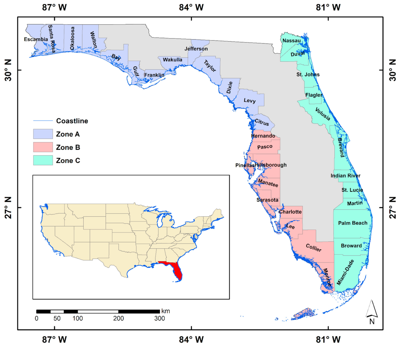
To facilitate spatiotemporal analyses, we classified the 35 coastal counties as three zones according to Florida Department of Environmental Protection [48] (Figure 2):
- Zone A: The Florida Panhandle, including the counties of Escambia, Santa Rosa, Okaloosa, Walton, Bay, Gulf, Franklin, Wakulla, Jefferson, Taylor, Dixie, Levy, and Citrus.
- Zone B: The Southwest Florida Gulf, including the counties of Hernando, Pasco, Pinellas, Hillsborough, Manatee, Sarasota, Charlotte, Lee, Collier, and Monroe.
- Zone C: The Atlantic Ocean, including the counties of Miami-Dade, Broward, Palm Beach, Martin, St. Lucie, Indian River, Brevard, Volusia, Flagler, St. Johns, Duval, and Nassau.
2.2. Data Preparation
The data are from the authors’ previous study [16], which produced the annual tidal flat maps from 1984 to 2020 with 30 m spatial resolution throughout the conterminous US. For Florida, a total of 17,163 Landsat 4, 5, 7, and 8 images, which were acquired every 16 days during these 37 years, were used to generate the annual maps for further analyses in this study. An RF model built on GEE [16] was used to process these satellite imageries, which classifies the pixels as five categories, including permanent water, tidal flats, vegetated lands, artificial surfaces, and barren grounds. The RF classification relies on the spectral change patterns between the Landsat imageries, and a total of one band and four spectrum-derived indices were utilized in this model, including shortwave infrared (SWIR) band, Automated Water Extraction Index (AWEI) [49], Normalized Difference Water Index (NDWI) [50], Soil Brightness (SB) [51], and Enhanced Vegetation Index (EVI) [52,53]. The 37 annual maps of each zone have an overall accuracy of 91.4%, which lays a reliable foundation for further analyses. In the classified results, the three dryland classes (vegetated lands, artificial surfaces, and barren grounds) were merged as a single class (lands), and the spatiotemporal dynamic analyses in the following sections were implemented on the three classes (permanent water, tidal flats, and lands).
2.3. Pixel Level Analysis
Recall that every pixel in the classified map has 30 m spatial resolution, a primary consideration is to find the area of tidal flats by year and explore the temporal change patterns by zone. On the other hand, the tidal flat occurrence map of each zone can be synthesized from all 37 years’ tidal flat distributions, in which the raster values vary from 0 (without occurrence) to 37 (always occurrence) [25]. To quantify the spatial features on the synthesized map, we also calculated the area of tidal flats weighted by the frequency during the 37 years, which are summarized by longitude and latitude, and displayed as line charts along map edges. Moreover, the tidal flat occurrence distributions were summarized as a line chart, which could provide another perspective to observe the temporal characteristics of tidal flat dynamics.
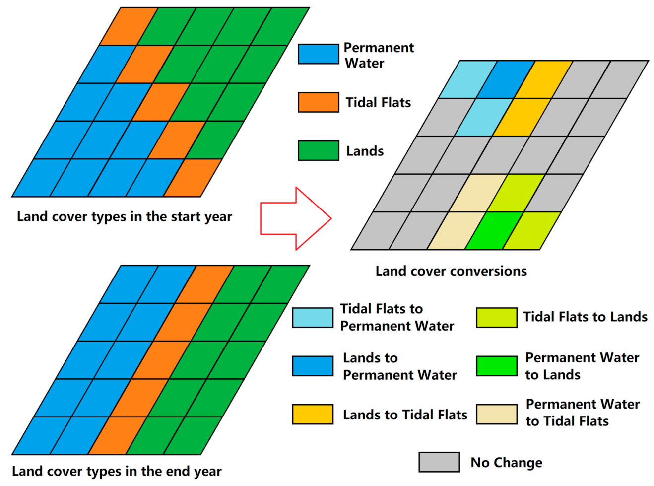
An in-depth consideration is to explore the interactions between tidal flats and two other land cover classes [8,9,17]. In this study, a total of six types of pixel-wise land cover conversions could be found by overlapping and comparing the maps of two years (Figure 3), and we only considered four of them which are directly related to tidal flats, including tidal flats to permanent water, tidal flats to lands, permanent water to tidal flats, and lands to tidal flats. Additionally, the unchanged tidal flat pixels appearing in two compared years were regarded as preserved tidal flats, which were also considered in this study. For temporal analysis, the land cover maps of consecutive years were overlapped and compared, which finds the areas of the five types of tidal flat interactions by year. In addition, an overlapping comparison was conducted between the earliest year (1984) and the most recent year (2020), which derives the maps for spatial assessments. To quantify the spatial distributions of the five types of tidal flat interactions, we again summarized the areas by longitude and latitude and displayed as line charts along map edges, in which the tidal flat losses (tidal flats to permanent water and tidal flats to lands) result in negative values, while tidal flat gains (permanent water to tidal flats and lands to tidal flats) result in positive values, and the preserved tidal flats correspond to zeros.
2.4. Object Level Assessment
A higher-level assessment for tidal flat dynamics is based on the objects [25]. As shown in Figure 3, one pixel may have up to eight neighboring pixels, and consequently the contiguous tidal flat pixels can be assembled as a whole entity, which refers to a tidal flat object [25]. Two geometry attributes of the derived objects can be used to examine the temporal characteristics of tidal flat dynamics, including:
- The average area of tidal flat objects: The converted data could be directly used to track the changes by zone throughout the 37 years.
- Weighted Polsby-Popper value [54]: The Polsby-Popper test is used to measure the compactness of the shape, which finds the ratio of the area of a tidal flat object to the area of a circle with the same perimeter as the tidal flat object and it varies from 0 (least compact) to 1 (most compact). In this study, an average value weighted by tidal flat object area was derived from each zone in each year, from which the temporal patterns of compactness changes could be identified.
2.5. Temporal Trends
This study applied an integrated nonparametric approach, which is widely used in GIS community [55,56,57,58,59,60,61,62,63], to identify and quantify the temporal trends of tidal flat dynamics. More specifically, it uses Mann–Kendall test [64,65] to determine the existence of a significant trend. If it exists (p-value is less than 0.05), use Sen’s slope estimator [66] to measure the magnitude of the trend. As a summary of the temporal analyses, this approach was applied to examine the trends of tidal flat area changes and the five types of tidal flat interactions on the pixel level, as well as the two attributes on the object level.
3. Results and Discussion
The analyses were based on the generated maps, and the results were illustrated and discussed in this section, including the pixel level (Section 3.1), object level (Section 3.2), and temporal trends (Section 3.3). In particular, the analytical results on the pixel level were divided into two parts, which are tidal flat dynamics (Section 3.1.1) and tidal flat interactions (Section 3.1.2).
3.1. Pixel Level
3.1.1. Tidal Flat Dynamics
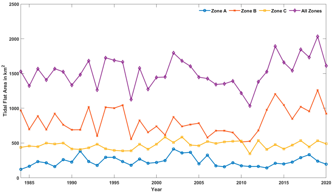
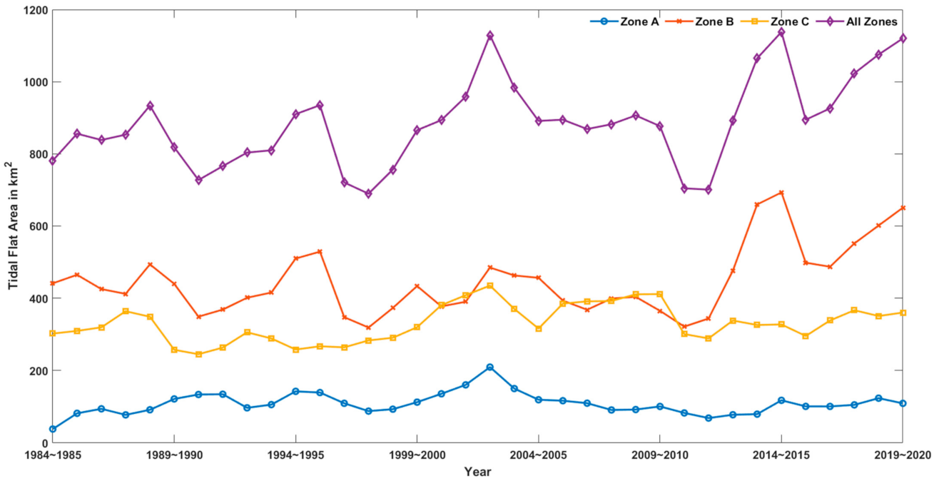
The temporal patterns of tidal flat area changes in the three zones and the whole study area were illustrated in Figure 4, which provides a preliminary observation for the tidal flat dynamics during the 37 years in Florida. By comparing the annual average area (µ) during the 37 years, Zone B has the highest area of tidal flats (µ = 812.73 km2), followed by Zone C (µ = 469.74 km2), and Zone A has the lowest area of tidal flats (µ = 235.99 km2), which are consistent with the observations from Figure 4. Considering the whole study area, the highest area of tidal flats was found in 2019 (2032.06 km2), which is nearly twice as much as that of the smallest record (1033.16 km2 in 2011). As illustrated in Figure 4, the tidal flat area in Zone B has a significant increase from 2011 (525.33 km2) to 2019 (1259.22 km2). It substantially contributed to the tidal flat expansions of the entire study area during those eight years, and the details will be discussed in the next subsection (Section 3.1.2). Additionally, in Zone B, we noticed a peak in 1992 (1017.32 km2), which is consistent with our previous study [25] and reconfirms that Hurricane Andrew (category 5) has brought in considerable sediments along the southwestern coast of Florida [38]. On the other hand, we observed two significant area decreases in Zone A, which are from 2004 (366.75 km2) to 2005 (201.45 km2) and from 2006 (326.02 km2) to 2007 (172.80 km2). According to the historical records [67], Zone A has experienced El Niño events during these two periods when the precipitations were significantly less than normal. As a result, the rivers have limited hydrodynamic forces and therefore may not provide sufficient sediments to the coastal area. Moreover, we examined the coefficient of variation (CV) by zones, which verified that the tidal flat area in Zone C (CV = 0.12) is more stable than that in Zone B (CV = 0.23), and the most variable tidal flats were found in Zone A (CV = 0.30). In summary, the CV of the whole study area equals to 0.14, which is close to that of Zone C but significantly less than those of Zone A and Zone B. Recall that Zone A and Zone B are both facing the Gulf of Mexico, while Zone C locates by the Atlantic Ocean, the CVs in the three zones highlight different characteristics between the two maritime spaces. As elucidated by a coastal study [46], the Gulf Coast is intensively affected by flooding and tidal inundations due to active storm events, which may explain the remarkable variances of tidal flat areas in Zone A and Zone B.
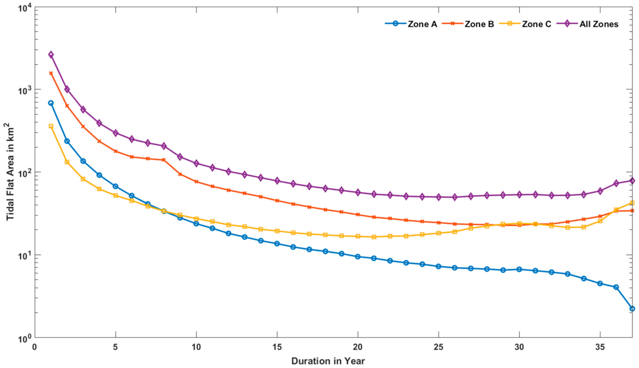
The tidal flat occurrence distributions in the three zones and the whole study area were summarized and illustrated in Figure 5, which provides another perspective to examine the temporal characteristics of tidal flat dynamics. As expected, the whole study area was dominantly occupied by short-endured (1 to 10 years) tidal flats (77.16%), while the long-endured (28 to 37 years) tidal flats held a negligible share (7.67%). It shows more significant patterns along the Gulf Coast, since the short-endured tidal flats contributed 84.94% of the area to Zone A and 79.97% of the area to Zone B, while the long-endured tidal flats contributed 3.31% of the area to Zone A and 5.90% of the area to Zone B. Unlike these two zones, Zone C had significantly larger share of long-endured tidal flats (18.09%), and therefore the short-endured tidal flats in Zone C (59.63%) held a much less share than the other two zones. It echoes the findings from Figure 4 and reconfirms that the tidal flats along the Gulf Coast are more vulnerable and dynamic, while the Atlantic Coast can provide a stable environment to maintain tidal flats for longer periods.
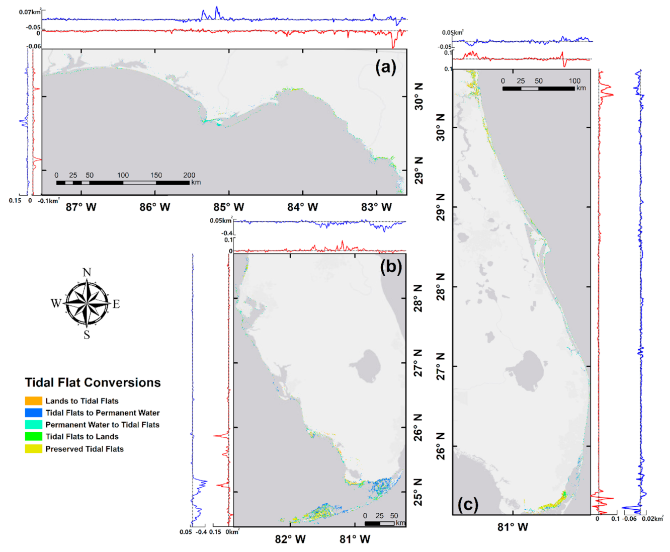
The spatial distributions of tidal flats were mapped and summarized in Figure 6, which provides a reference to identify the tidal flat clusters in the three zones. In Figure 6a, the horizonal line chart shows three major peaks (up to 4 km2), which correspond to two clusters in Zone A. The first one locates at the estuary of Apalachicola River, which can be found around the center of the map. On one hand, the barrier islands separate the lagoon from the Gulf of Mexico, which contribute to an advantageous environment for sediment maintenances [68]. On the other hand, the Apalachicola River is continuously providing fine-grained sediments around its estuary and therefore has become a major resource of tidal flat accretions [69]. Another major cluster in this zone can be found from the east portion, which is also known as Florida’s Big Bend Coast and under the administrations by multiple authorities, including but not limited to Flint Rock Wildlife Management Area, Big Bend Wildlife Management Area, Tide Swamp Wildlife Management Area, and Waccasassa Bay Preserve State Park. These places are famous for salt marshes and tidal creeks, which restrict visitation and remain undeveloped according to the state laws. The Big Bend Coast has “one of the last remaining remnants of the once vast Gulf Hammock” and plays an essential role in the biodiversity and ecological sustainability of Northwestern Florida [70]. In Figure 6b, a secondary peak (less than 10 km2) was found at the left end of the horizontal line chart, which identifies a cluster around the northwestern corner of Zone B. Geologically, it is an extension of the Big Bend Coast, and the Weeki Wachee River plays a key role in sediment depositing for this area [71]. More importantly, the major peaks (up to 20 km2) were found from the lower portion of the vertical line chart, which correspond to the clusters in Everglades National Park and Florida Keys. The Everglades National Park and the surrounding area constitute a huge slough system, which carries the muds from inland to seaside [72] and consequently deposits substantial sediments over salt marshes and tidal creeks [73]. On the other hand, the seabed around Florida Keys is featured by migrating tidal bars, which are alternatively exposed or inundated during the tidal cycles, and the sand waves driven by the strong reversing tidal currents constitute a unique environment to boost the sediment depositions [74]. In Figure 6c, a major peak (up to 20 km2) was observed at the lower end of the vertical line chart, which identifies the cluster in the southeastern portion of the Everglades National Park. In addition, a secondary peak (less than 10 km2) was found at the upper end of the vertical line chart, which highlights a cluster in the northmost section of Florida’s Atlantic Coast. This cluster corresponds to the Timucuan Ecological and Historical Preserve, which administrates an estuary system strongly influenced by the interactions between land and sea. This ecological and historical preserve, together with the coastal areas in Georgia and South Carolina, constitute a huge wetland ecosystem along the Atlantic Coast [75]. These maps and line charts confirm that Zone B has the largest tidal flats, followed by Zone C, and Zone A has the least distributions, which echo the findings from Figure 4.
3.1.2. Tidal Flat Interactions
In this subsection, we firstly explored the temporal change patterns of the preserved tidal flats according to the results illustrated in Figure 7. Although Zone B has the largest preserved tidal flats in most cases, some periods such as 2001 to 2002, 2006 to 2007, and 2009 to 2010 have demonstrated larger preserved tidal flats in Zone C than Zone B, which suggests that the tidal flats in Zone B are more variable than those in Zone C. It means that unusually high area of tidal flats in Zone B interacted with other land cover types during these three periods. Regarding the annual averages, the preserved tidal flats have contributed 46.05% (108.68 km2) of the total tidal flat area in Zone A, 55.05% (447.37 km2) in Zone B, 70.22% (329.85 km2) in Zone C, and consequently 58.38% (885.90 km2) in the whole study area. On the other hand, the CV of the preserved tidal flat area is 0.27 in Zone A, 0.21 in Zone B, and 0.15 in Zone C. Therefore, Zone C has the most stable tidal flats, while the most variable tidal flats are in Zone A. It echoes the findings from Figure 5, as Zone C has the largest share of long-endured tidal flats and the least share of short-endured tidal flats among the three zones, while Zone A is in the reverse case.
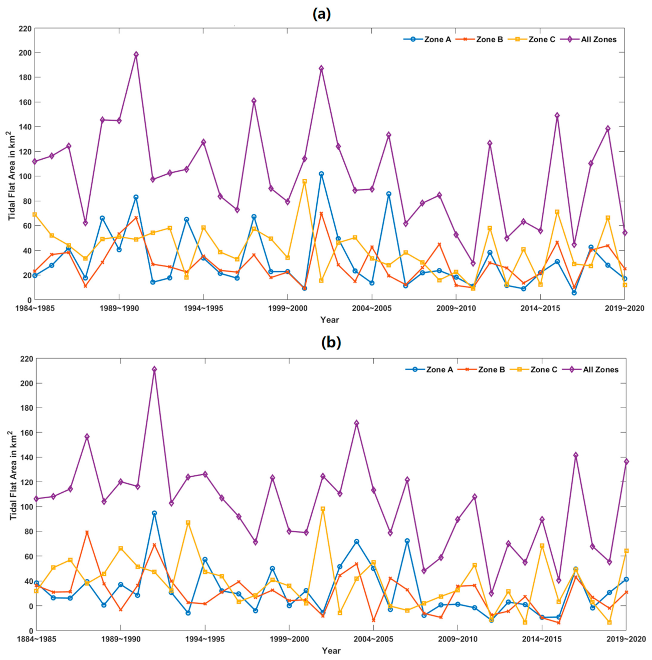
Secondly, the interactions between tidal flats and lands were investigated based on the temporal change patterns given by Figure 8. On 37 years’ average, the rates of lands converted to tidal flats are 32.05 km2 per year in Zone A, 28.91 km2 per year in Zone B, 40.64 km2 per year in Zone C, and consequently 101.60 km2 per year in the whole study area. The reverse cases, which refer to the annual average rates of tidal flats converted to lands, are 32.12 km2 per year in Zone A, 30.03 km2 per year in Zone B, 39.17 km2 per year in Zone C, and consequently 101.32 km2 per year in the whole study area. Unlike the results in the previous sections, none of the three zones have demonstrated significantly larger or smaller tidal flat area that converted from or to lands than two other zones, and hence the zone rankings in the two subfigures vary from year to year. Particularly, Figure 8a demonstrates that Zone B has higher area than Zone C from 2001 to 2002, from 2004 to 2005, and from 2008 to 2009. Meanwhile, Figure 8b illustrates that Zone B has higher area than Zone C from 2005 to 2007 and from 2009 to 2010. It echoes the three periods identified in Figure 7 and further substantiates that the tidal flats in Zone B had unusually active interactions with lands during these periods. On the other hand, the rate of net interactions between tidal flats and lands in each zone can be found by comparing the annual average rates of the two conversions between them. As a result, it shows that the tidal flats in Zone A have lost to lands at the rate of 0.07 km2 per year, and the losing rate in Zone B is 1.12 km2 per year, while the tidal flats in Zone C have gained from lands at the rate of 1.47 km2 per year. It suggests that the Gulf Coast of Florida has been facing environmental challenges from the landward side, while the environment of Florida’s Atlantic Coast is more stable and healthier. The environmental crisis of Florida’s Gulf Coast has been confirmed by a recent study [76], which figures that the rapid deforestation has critically undermined the sustainability of the coastal environment in this area.
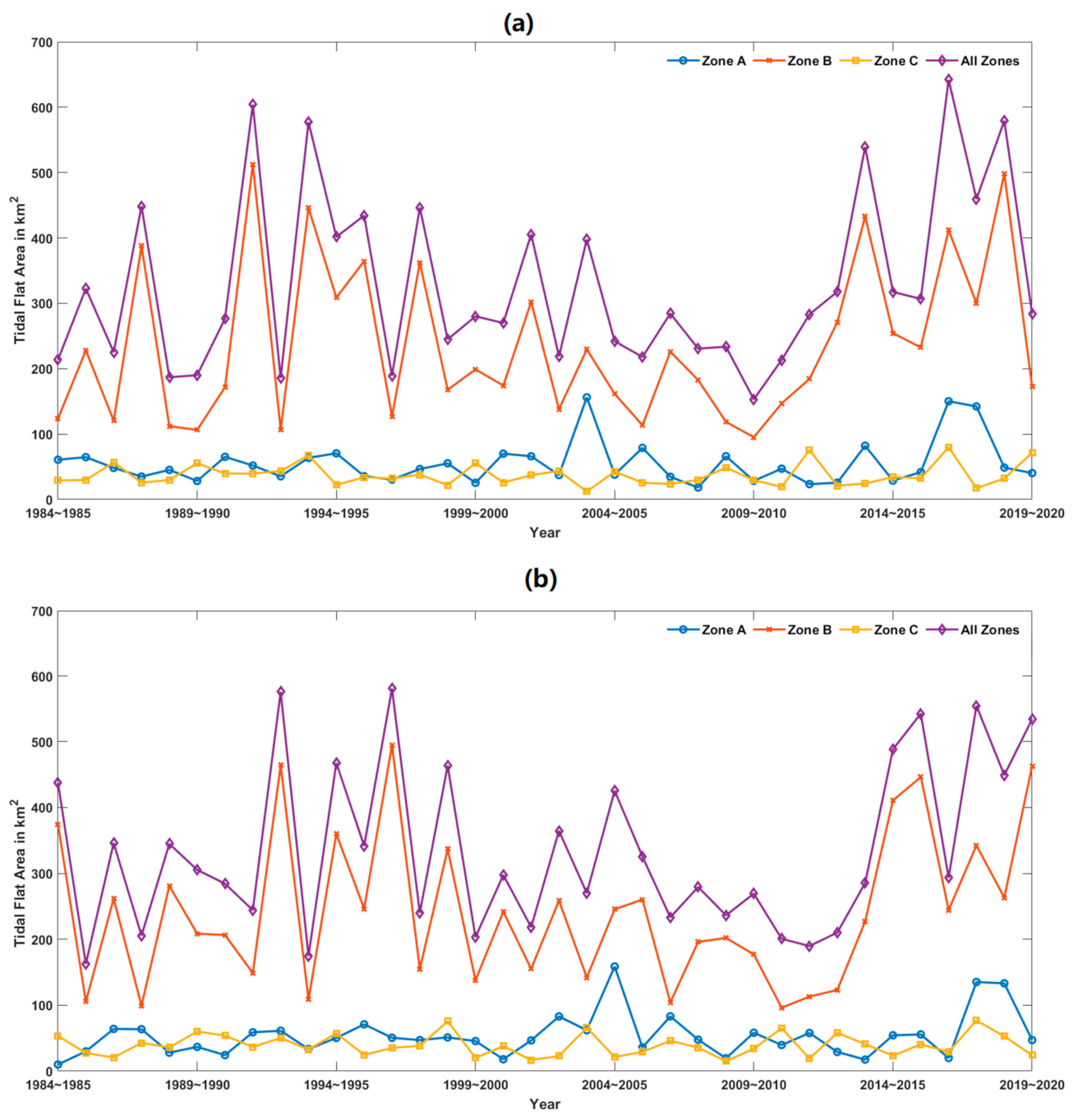
Thirdly, the interactions between tidal flats and permanent water were visualized as Figure 9. In contrast to Figure 8, these two subfigures explicitly illustrate that Zone B has larger tidal flats involved in the interactions with permanent water than two other zones and therefore dominates the total area changes throughout the study area. On annual average, the rates of permanent water converted to tidal flats are 55.19 km2 per year in Zone A, 235.83 km2 per year in Zone B, 34.70 km2 per year in Zone C, and in summary 328.42 km2 per year in the whole study area. On the other hand, the annual average rates of tidal flats converted to permanent water are 53.49 km2 per year in Zone A, 241.61 km2 per year in Zone B, 34.37 km2 per year in Zone C, and in summary 334.47 km2 per year in the whole study area. Regarding the net interactions, tidal flats have gained from permanent water at the average rates of 1.70 km2 per year in Zone A and 0.33 km2 per year in Zone C, while lost to permanent water at the average rate of 5.78 km2 per year in Zone B. The results warn that a large portion of the tidal flats in Zone B have been inundated and therefore the coastal environment in this zone calls for higher awareness and further protections. As confirmed by another study [77], the mangrove forest along the southern Florida coast has been rapidly lost due to climate change, which makes the coastal area more vulnerable to the effects of sea-level rise.
Lastly, the result of overlapping comparison between the earliest year and most recent year was illustrated as Figure 10. Accordingly, the discussion was divided into two parts based on the two parallel sets of line charts, and the first part investigated the interactions between tidal flats and lands (summarized as red line charts). In Figure 10a, a secondary valley was found from the upper portion of the vertical line chart (about −0.08 km2), which corresponds to the coast administrated by Flint Rock Wildlife Management Area. More importantly, the major valleys were identified from both the lower portion of the vertical line chart (up to −0.1 km2) and the right end of the horizonal line chart (up to −0.06 km2), which highlights the intensified losses of tidal flats in Waccasassa Bay Preserve State Park. The above two places are both located along the Big Bend Coast, and the landward retreats of tidal flats highlight the environmental concerns in this area. This finding is consistent with another study [78], which identified the rapid, sustained, and irreversible loss of forests along the Big Bend Coast due to climate change. In Figure 10b, a major peak (up to 0.15 km2) and a secondary peak (up to 0.1 km2) were identified from the lower portion of the vertical line chart, which correspond to the Ten Thousand Islands and Flamingo Beach in the Everglades National Park. Since 2000, the Comprehensive Everglades Restoration Plan initiated by the federal government of the US has largely contributed to the ecological restoration in the Everglades National Park [79], and the previous studies [80,81] have confirmed the significant resilience of marshes and mangrove forests in the two places identified above. In Figure 10c, the map observes large clusters of preserved tidal flats, and the vertical line chart identified fluctuations around the lower end and peaks around the upper end. The fluctuations correspond to Turkey Point Nuclear Generating Station, which locates at the southeastern corner of Miami-Dade County and has a huge cooling canal system next to the clusters of tidal flats in the Everglades National Park. Due to the limitation of Landsat data in the early years, the canal network may cause minor errors on the classified map of 1984 and consequently slightly affect the result of overlapping comparison between 1984 and 2020 (up to 0.03 km2). As a result, the focus in Zone C is to analyze the northmost cluster instead, which refers to Timucuan Ecological and Historical Preserve. The corresponding peaks on the vertical line chart indicated the substantial resilience of the coastal environment, which echoes the previous study [82] and endorses the environmental prevention strategies taken by the local authority.
In the second part, we analyzed the interactions between tidal flats and permanent water (summarized as blue line charts). In Figure 10a, the major peaks were detected from the vertical line chart (up to 0.15 km2) and the horizonal line chart (0.07 km2), and they both correspond to the tidal flat cluster around the estuary of Apalachicola River. It suggests that the river has brought in and deposited substantial sediments, which extend the outer margin of tidal flats off the coast. The similar phenomena were also observed around the estuaries of Yellow River and Yangtze River in China [2], which verified that rivers could dominate the activities of tidal flats around the estuaries. In Figure 10b, the major valleys were detected from the lower portion of the vertical line chart, and accordingly the large clusters of tidal flats converted to permanent water were found from Florida Bay and the north edge of Lower Florida Keys. On one hand, the mortality of seagrass undermined the stability of the coast, which accelerated the margin erosion in Florida Bay [83]. On the other hand, sea level rise is becoming a major concern to this area, and in particular the Lower Florida Keys have demonstrated higher risk of inundation [84]. In Figure 10c, the vertical line chart shows a valley around the lower end, which substantiates that the adjacent area of Florida Bay in Zone C has experienced a tidal flat loss as Zone B has. By contrast, this subfigure could not detect any other significant interactions between tidal flats and permanent water, which is consistent with Figure 9 as it demonstrated much smaller tidal flats in Zone C interacted with the permanent water than two other zones.
3.2. Object Level
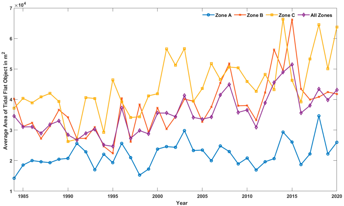
The first attribute of tidal flats on this level is the average area of objects, and the annual change patterns by zone were illustrated in Figure 11. As shown, Zone C has the largest tidal flat objects on the 37 years’ average (44,589 m2), which is followed by Zone B (37,322 m2) and Zone A (21,936 m2). This ranking contradicts the findings from Figure 4, in which Zone B shown the largest tidal flat area among the three zones. This inconsistency implies that the tidal flat distribution in Zone B is more scattered and consequently there are more tidal flat objects in this zone, while the distribution in Zone C is more concentrated and therefore it has fewer tidal flat objects. In addition, Figure 11 observes a strong correlation between Zone B and the whole study area, which was verified by Pearson correlation test (r = 0.913). Regarding the annual averages, the tidal flat objects are most distributed in Zone B (758,367), while the other two zones have much fewer objects (346,711 in Zone A and 355,276 in Zone C), which echoes the previous findings and suggests that Zone B dominates the statistics on this level owing to the large number of tidal flat objects.
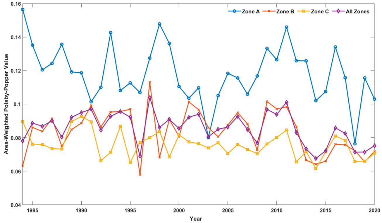
The next attribute to be analyzed is the area-weighted Polsby-Popper value, and the temporal dynamic information was summarized by zones and visualized as Figure 12. Tidal flats are the buffer zones between land and sea [1], so the smaller objects are more likely to be regular shapes with greater compactness, while the larger objects are more likely to be narrow shapes with less compactness scattered along the coast. Regarding the average values during the 37 years, Zone A had the most compact tidal flat objects (0.118), followed by Zone B (0.084), and the least compact tidal flat objects were found in Zone C (0.076), which follows a reversed ranking order of the first attribute and is in line with expectations. Again, a strong statistical relationship between Zone B and the whole study area was verified by Pearson correlation test (r = 0.914), which echoes the findings from the previous attribute. The two attributes on the object level could provide an in-depth observation for the tidal flat dynamics throughout the study area, which is invisible on the pixel level.
3.3. Temporal Trends
Based on time-series datasets, this section identified the temporal trends of tidal flat dynamics on both two levels by zones. First, the trends on the pixel level were summarized as Table 1, including the total area of tidal flats (Figure 4), the area of preserved tidal flats (Figure 7), the area of tidal flats interacted with lands (Figure 8), and with permanent water (Figure 9). As shown in Table 1, we could not identify any trend from Zone A and Zone B, while captured significant trends from Zone C and the whole study area in terms of the preserved tidal flats as well as the tidal flats interacted with lands. Specifically speaking, the preserved tidal flats were continuously growing during the 37 years at the rates of 2.302 km2/year in Zone C and 5.160 km2/year in the whole study area, which indicates that the tidal flats throughout the whole study area, especially in Zone C, were becoming stable. It echoes the findings from Figure 5, which demonstrates that Zone C has significantly larger share of long-endured tidal flats than the other two zones and consequently increases the proportion of long-endured tidal flats throughout the study area. Regarding the interactions between tidal flats and lands, the two conversion types observed declining trends in both Zone C and the whole study area. It suggests that the stabilities of tidal flats during the 37 years throughout the whole study area, particularly in Zone C, largely relied on the landward side rather than seaward side. In other words, compared with the environmental challenges from the ocean, including but not limited sea level rise, storms, and hurricanes [85], the threats to tidal flats from the lands are relatively less. This finding not only recognizes the achievements by Florida Coastal Management Program [86] along the Atlantic Coast, but also highlights that the significant progresses along the Gulf Coast are yet to come and therefore it calls for more efforts and more practical strategies.
Second, the trends on the object level were summarized as Table 2, including the average area of tidal flat objects (Figure 11) and the area-weighted Polsby-Popper value (Figure 12). Again, the significant trends of two attributes were identified from both Zone C and the whole study area, and additionally the average area of tidal flat objects in Zone B also demonstrated a significant trend. To be more specific, the average area of tidal flat objects throughout the study area observed a continuous expansion during the 37 years at the rate of 444.51 m2/year, which is mainly driven by Zone B (498.74 m2/year) and Zone C (504.50 m2/year). Regarding the area-weighted Polsby-Popper value, the declining trends were identified from both Zone C (−0.0003 per year) and the whole study area (−0.0004 per year). It means that the expansions of tidal flat objects throughout the study area, especially in Zone C, have more directionalities than symmetries. This finding is anticipated, as the shapes of tidal flat objects are determined by topographical factors and consequently should not be regular.
4. Conclusions
This study implemented a series of spatiotemporal analyses on tidal flats along the coast of Florida from 1984 to 2020, which consist of the assessments on the two levels. The results highlight the differences in tidal flat distributions and dynamics between the two maritime spaces. While the tidal flats are more distributed along the Gulf Coast, they demonstrate more vulnerable characteristics and therefore call for higher level of awareness and protections. By contrast, the Atlantic Coast has less tidal flats, but it could provide a stable environment for the maintenance and accretion of tidal flats.
As one of the earliest studies aiming at the dynamics of tidal flats throughout Florida, this paper systematically analyzed the change patterns on the large spatiotemporal scale. It does not consider the dynamics of the study subject only, but instead provides insights into the multi-level perspective and the comprehensive analytical strategy of considering the interactions with other subjects. Compared with the conventional methods, the innovative GIS representations and analyses can derive more diversified information, which could be utilized to better track and describe the change patterns of dynamic geographic phenomena on large spatiotemporal scales.
As we implemented a successful case study in Florida, this framework could be applied to the whole US, and we can conduct a series of follow-up studies. First, we are interested in investigating the correlations between tidal flat dynamics and other factors, including but not limited to storm events, estuary sedimentations, sea-level rises, and coastal constructions. Second, the lifecycle modeling is considered to be another direction of future work. It is the third level of dynamic analysis, which identifies the filiations between the objects at adjacent time steps and links them as chains [23,24,25]. On this level, a variety of events will be defined to better capture and describe the dynamic activities of tidal flats, including splitting, merger, continuation, and so on.
Author Contributions
Conceptualization, W.L. and C.X.; methodology, C.X. and W.L.; software, C.X.; formal analysis, C.X. and W.L.; writing—original draft preparation, C.X.; writing—review and editing, W.L.; supervision, W.L. All authors have read and agreed to the published version of the manuscript.
Funding
This research received no external funding.
Institutional Review Board Statement
Not applicable.
Informed Consent Statement
Not applicable.
Data Availability Statement
Publicly available datasets were analyzed in this study. This data can be found here: https://developers.google.com/earth-engine/datasets/ (accessed on 13 November 2021).
Acknowledgments
We would like to thank the four anonymous reviewers and editors for providing valuable comments and suggestions which helped improve the manuscript greatly.
Conflicts of Interest
The authors declare no conflict of interest.
References
- Gao, S. Geomorphology and sedimentology of tidal flats. In Coastal Wetlands; Elsevier: Amsterdam, The Netherlands, 2019; pp. 359–381. [Google Scholar]
- Wang, X.; Xiao, X.; Zou, Z.; Chen, B.; Ma, J.; Dong, J.; Li, B. Tracking annual changes of coastal tidal flats in China during 1986–2016 through analyses of Landsat images with Google Earth Engine. Remote Sens. Environ. 2020, 238, 110987. [Google Scholar] [CrossRef]
- Wang, X.; Xiao, X.; Zou, Z.; Hou, L.; Qin, Y.; Dong, J.; Li, B. Mapping coastal wetlands of China using time series Landsat images in 2018 and Google Earth Engine. ISPRS J. Photogramm. Remote Sens. 2020, 163, 312–326. [Google Scholar] [CrossRef]
- Mullarney, J.C.; Henderson, S.M.; Reyns, J.A.; Norris, B.K.; Bryan, K.R. Spatially varying drag within a wave-exposed mangrove forest and on the adjacent tidal flat. Cont. Shelf Res. 2017, 147, 102–113. [Google Scholar] [CrossRef]
- Reed, D.; van Wesenbeeck, B.; Herman, P.M.; Meselhe, E. Tidal flat-wetland systems as flood defenses: Understanding biogeomorphic controls. Estuar. Coast. Shelf Sci. 2018, 213, 269–282. [Google Scholar] [CrossRef]
- Choi, Y.R. Profitable tidal flats, governable fishing communities: Assembling tidal flat fisheries in post-crisis South Korea. Political Geogr. 2019, 72, 20–30. [Google Scholar] [CrossRef]
- Xu, M.; Cui, B.; Lan, S.; Li, D.; Wang, Y.; Jiang, B. Exploring dynamic change of the tidal flat aquaculture area in the shandong peninsula (China) using multitemporal landsat imagery (1990–2015). J. Coast. Res. 2020, 99, 197–202. [Google Scholar] [CrossRef]
- Cao, W.; Zhou, Y.; Li, R.; Li, X. Mapping changes in coastlines and tidal flats in developing islands using the full time series of Landsat images. Remote Sens. Environ. 2020, 239, 111665. [Google Scholar] [CrossRef]
- Cao, W.; Zhou, Y.; Li, R.; Li, X.; Zhang, H. Monitoring long-term annual urban expansion (1986–2017) in the largest archipelago of China. Sci. Total Environ. 2021, 776, 146015. [Google Scholar] [CrossRef]
- Miththapala, S. Tidal Flats; Coastal Ecosystems Series; IUCN: Colombo, Sri Lanka, 2013; Volume 5. [Google Scholar]
- Rifat, S.A.A.; Liu, W. Measuring community disaster resilience in the conterminous coastal United States. ISPRS Int. J. Geo-Inf. 2020, 9, 469. [Google Scholar] [CrossRef]
- Murray, N.J.; Phinn, S.R.; DeWitt, M.; Ferrari, R.; Johnston, R.; Lyons, M.B.; Fuller, R.A. The global distribution and trajectory of tidal flats. Nature 2019, 565, 222–225. [Google Scholar] [CrossRef]
- Jia, M.; Wang, Z.; Mao, D.; Ren, C.; Wang, C.; Wang, Y. Rapid, robust, and automated mapping of tidal flats in China using time series Sentinel-2 images and Google Earth Engine. Remote Sens. Environ. 2021, 255, 112285. [Google Scholar] [CrossRef]
- Otsu, N. A threshold selection method from gray-level histograms. IEEE Trans. Syst. Man Cybern. 1979, 9, 62–66. [Google Scholar] [CrossRef] [Green Version]
- Zhang, K.; Dong, X.; Liu, Z.; Gao, W.; Hu, Z.; Wu, G. Mapping tidal flats with Landsat 8 images and google earth engine: A case study of the China’s eastern coastal zone circa 2015. Remote Sens. 2019, 11, 924. [Google Scholar] [CrossRef] [Green Version]
- Xu, C.; Liu, W. Mapping and analyzing the annual dynamics of tidal flats in the conterminous United States during 1984 to 2020 using Google Earth Engine. Environ. Adv. 2021. submitted. [Google Scholar]
- Hu, Y.; Zhang, Y. Spatial–temporal dynamics and driving factor analysis of urban ecological land in Zhuhai city, China. Sci. Rep. 2020, 10, 16174. [Google Scholar] [CrossRef]
- Cao, W.; Li, R.; Chi, X.; Chen, N.; Chen, J.; Zhang, H.; Zhang, F. Island urbanization and its ecological consequences: A case study in the Zhoushan Island, East China. Ecol. Indic. 2017, 76, 1–14. [Google Scholar] [CrossRef]
- Ahlqvist, O.; Bibby, P.; Duckham, M.; Fisher, P.; Harvey, F.; Schuurman, N. Not just objects: Reconstructing objects. In Re-Presenting GIS; John Wiley & Sons: London, UK, 2005; pp. 17–25. [Google Scholar]
- Blaschke, T.; Hay, G.J.; Kelly, M.; Lang, S.; Hofmann, P.; Addink, E.; Tiede, D. Geographic object-based image analysis—Towards a new paradigm. ISPRS J. Photogramm. Remote Sens. 2014, 87, 180–191. [Google Scholar] [CrossRef] [Green Version]
- Couclelis, H. People manipulate objects (but cultivate fields): Beyond the raster-vector debate in GIS. In Theories and Methods of Spatio-Temporal Reasoning in Geographic Space; Springer: Berlin/Heidelberg, Germany, 1992; pp. 65–77. [Google Scholar]
- Goodchild, M.F.; Yuan, M.; Cova, T.J. Towards a general theory of geographic representation in GIS. Int. J. Geogr. Inf. Sci. 2007, 21, 239–260. [Google Scholar] [CrossRef] [Green Version]
- Liu, W.; Li, X.; Rahn, D.A. Storm event representation and analysis based on a directed spatiotemporal graph model. Int. J. Geogr. Inf. Sci. 2016, 30, 948–969. [Google Scholar] [CrossRef]
- Zhu, R.; Guilbert, E.; Wong, M.S. Object-oriented tracking of the dynamic behavior of urban heat islands. Int. J. Geogr. Inf. Sci. 2017, 31, 405–424. [Google Scholar] [CrossRef] [Green Version]
- Xu, C.; Liu, W. Integrating a Three-Level GIS Framework and a Graph Model to Track, Represent, and Analyze the Dynamic Activities of Tidal Flats. ISPRS Int. J. Geo-Inf. 2021, 10, 61. [Google Scholar] [CrossRef]
- Central Intelligence Agency. Coastline. The World Factbook. 2021. Available online: https://www.cia.gov/the-world-factbook/field/coastline/ (accessed on 13 November 2021).
- Lamb, B.T.; Tzortziou, M.A.; McDonald, K.C. Evaluation of approaches for mapping tidal wetlands of the chesapeake and delaware bays. Remote Sens. 2019, 11, 2366. [Google Scholar] [CrossRef] [Green Version]
- Ballanti, L.; Byrd, K.B.; Woo, I.; Ellings, C. Remote sensing for wetland mapping and historical change detection at the nisqually river delta. Sustainability 2017, 9, 1919. [Google Scholar] [CrossRef] [Green Version]
- Li, W.; Gong, P. Continuous monitoring of coastline dynamics in western Florida with a 30-year time series of landsat imagery. Remote Sens. Environ. 2016, 179, 196–209. [Google Scholar] [CrossRef]
- Ghosh, S.; Mishra, D.R.; Gitelson, A.A. Long-term monitoring of biophysical characteristics of tidal wetlands in the northern Gulf of Mexico—A methodological approach using MODIS. Remote Sens. Environ. 2016, 173, 39–58. [Google Scholar] [CrossRef] [Green Version]
- National Oceanic and Atmospheric Administration. Shoreline Mileage of the United States. NOAA Shoreline Website. 2021. Available online: https://coast.noaa.gov/data/docs/states/shorelines.pdf (accessed on 13 November 2021).
- United States Census Bureau. Resident Population for the 50 States, the District of Columbia, and Puerto Rico: 2020 Census. 2020 Census Apportionment Results. 2021. Available online: https://www2.census.gov/programs-surveys/decennial/2020/data/apportionment/apportionment-2020-table02.pdf (accessed on 13 November 2021).
- United States Census Bureau. Annual Resident Population Estimates, Estimated Components of Resident Population Change, and Rates of the Components of Resident Population Change for States and Counties: April 1, 2010 to July 1, 2020. County Population Totals: 2010–2020. 2020. Available online: https://www.census.gov/programs-surveys/popest/technical-documentation/research/evaluation-estimates/2020-evaluation-estimates/2010s-counties-total.html (accessed on 13 November 2021).
- Peel, M.C.; Finlayson, B.L.; McMahon, T.A. Updated world map of the Köppen-Geiger climate classification. Hydrol. Earth Syst. Sci. 2007, 11, 1633–1644. [Google Scholar] [CrossRef] [Green Version]
- Scott, T.M.; Campbell, K.M.; Rupert, F.R.; Arthur, J.D.; Missimer, T.M.; Lloyd, J.M.; Yon, J.W.; Duncan, J.G. Geologic Map of the State of Florida; Florida Geological Survey: Tallahassee, FL, USA, 2001. [Google Scholar]
- Malmstadt, J.; Scheitlin, K.; Elsner, J. Florida hurricanes and damage costs. Southeast. Geogr. 2009, 49, 108–131. [Google Scholar] [CrossRef]
- Davis, S.E., III; Cable, J.E.; Childers, D.L.; Coronado-Molina, C.; Day, J.W., Jr.; Hittle, C.D.; Sklar, F. Importance of storm events in controlling ecosystem structure and function in a Florida gulf coast estuary. J. Coast. Res. 2004, 20, 1198–1208. [Google Scholar] [CrossRef]
- Risi, J.A.; Wanless, H.R.; Tedesco, L.P.; Gelsanliter, S. Catastrophic sedimentation from Hurricane Andrew along the southwest Florida coast. J. Coast. Res. 1995, 83–102. Available online: https://0-www-jstor-org.brum.beds.ac.uk/stable/25736002 (accessed on 13 November 2021).
- Breithaupt, J.L.; Hurst, N.; Steinmuller, H.E.; Duga, E.; Smoak, J.M.; Kominoski, J.S.; Chambers, L.G. Comparing the biogeochemistry of storm surge sediments and pre-storm soils in coastal wetlands: Hurricane Irma and the Florida Everglades. Estuaries Coasts 2020, 43, 1090–1103. [Google Scholar] [CrossRef]
- Liu, K.; Chen, Q.; Hu, K.; Xu, K.; Twilley, R.R. Modeling hurricane-induced wetland-bay and bay-shelf sediment fluxes. Coast. Eng. 2018, 135, 77–90. [Google Scholar] [CrossRef]
- Zang, Z.; Xue, Z.G.; Xu, K.; Bentley, S.J.; Chen, Q.; D’Sa, E.J.; Ou, Y. The role of sediment-induced light attenuation on primary production during Hurricane Gustav (2008). Biogeosciences 2020, 17, 5043–5055. [Google Scholar] [CrossRef]
- Bianucci, L.; Balaguru, K.; Smith, R.W.; Leung, L.R.; Moriarty, J.M. Contribution of hurricane-induced sediment resuspension to coastal oxygen dynamics. Sci. Rep. 2018, 8, 15740. [Google Scholar] [CrossRef] [PubMed] [Green Version]
- Takesue, R.K.; Sherman, C.; Ramirez, N.I.; Reyes, A.O.; Cheriton, O.M.; Ríos, R.V.; Storlazzi, C.D. Land-based sediment sources and transport to southwest Puerto Rico coral reefs after Hurricane Maria, May 2017 to June 2018. Estuar. Coast. Shelf Sci. 2021, 259, 107476. [Google Scholar] [CrossRef]
- Ramos-Scharrón, C.E.; Arima, E.Y.; Guidry, A.; Ruffe, D.; Vest, B. Sediment mobilization by hurricane-driven shallow landsliding in a wet subtropical watershed. J. Geophys. Res. Earth Surf. 2021, 126, e2020JF006054. [Google Scholar] [CrossRef]
- Borchert, S.M.; Osland, M.J.; Enwright, N.M.; Griffith, K.T. Coastal wetland adaptation to sea level rise: Quantifying potential for landward migration and coastal squeeze. J. Appl. Ecol. 2018, 55, 2876–2887. [Google Scholar] [CrossRef]
- Mendelssohn, I.A.; Byrnes, M.R.; Kneib, R.T.; Vittor, B.A. Coastal habitats of the Gulf of Mexico. In Habitats and Biota of the Gulf of Mexico: Before the Deepwater Horizon Oil Spill; Springer: New York, NY, USA, 2017; pp. 359–640. [Google Scholar]
- Komar, P.D. Beach processes and erosion—An introduction. In CRC Handbook of Coastal Processes and Erosion; CRC Press: Boca Raton, FL, USA, 2018; pp. 1–20. [Google Scholar]
- Florida Department of Environmental Protection. Florida Coastal Access Guide. Resilience and Coastal Protection. 2020. Available online: https://floridadep.gov/rcp/coastal-access-guide/content/florida-coastal-access-guide (accessed on 13 November 2021).
- Feyisa, G.L.; Meilby, H.; Fensholt, R.; Proud, S.R. Automated Water Extraction Index: A new technique for surface water mapping using Landsat imagery. Remote Sens. Environ. 2014, 140, 23–35. [Google Scholar] [CrossRef]
- McFeeters, S.K. The use of the normalized difference water index (NDWI) in the delineation of open water features. Int. J. Remote Sens. 1996, 17, 1425–1432. [Google Scholar] [CrossRef]
- Baig, M.H.A.; Zhang, L.; Shuai, T.; Tong, Q. Derivation of a tasselled cap transformation based on Landsat 8 at-satellite reflectance. Remote Sens. Lett. 2014, 5, 423–431. [Google Scholar] [CrossRef]
- Huete, A.; Didan, K.; Miura, T.; Rodriguez, E.P.; Gao, X.; Ferreira, L.G. Overview of the radiometric and biophysical performance of the MODIS vegetation indices. Remote Sens. Environ. 2002, 83, 195–213. [Google Scholar] [CrossRef]
- Huete, A.R.; Liu, H.Q.; Batchily, K.V.; Van Leeuwen, W.J.D.A. A comparison of vegetation indices over a global set of TM images for EOS-MODIS. Remote Sens. Environ. 1997, 59, 440–451. [Google Scholar] [CrossRef]
- Polsby, D.D.; Popper, R.D. The third criterion: Compactness as a procedural safeguard against partisan gerrymandering. Yale Law Policy Rev. 1991, 9, 301–353. [Google Scholar] [CrossRef]
- Gocic, M.; Trajkovic, S. Analysis of changes in meteorological variables using Mann-Kendall and Sen’s slope estimator statistical tests in Serbia. Glob. Planet. Chang. 2013, 100, 172–182. [Google Scholar] [CrossRef]
- Da Silva, R.M.; Santos, C.A.; Moreira, M.; Corte-Real, J.; Silva, V.C.; Medeiros, I.C. Rainfall and river flow trends using Mann–Kendall and Sen’s slope estimator statistical tests in the Cobres River basin. Nat. Hazards 2015, 77, 1205–1221. [Google Scholar] [CrossRef]
- Diop, L.; Bodian, A.; Diallo, D. Spatiotemporal trend analysis of the mean annual rainfall in Senegal. Eur. Sci. J. 2016, 12, 231–245. [Google Scholar] [CrossRef]
- Peng, S.; Ding, Y.; Wen, Z.; Chen, Y.; Cao, Y.; Ren, J. Spatiotemporal change and trend analysis of potential evapotranspiration over the Loess Plateau of China during 2011–2100. Agric. For. Meteorol. 2017, 233, 183–194. [Google Scholar] [CrossRef] [Green Version]
- Minaei, M.; Irannezhad, M. Spatio-temporal trend analysis of precipitation, temperature, and river discharge in the northeast of Iran in recent decades. Theor. Appl. Climatol. 2018, 131, 167–179. [Google Scholar] [CrossRef]
- Gul, S.; Ren, J.; Zhu, Y.; Xiong, N.N. A systematic scheme for non-parametric spatio-temporal trend analysis about aridity index. In Proceedings of the 2020 IEEE International Conference on Systems, Man, and Cybernetics (SMC), Toronto, ON, Canada, 11–14 October 2020; pp. 981–986. [Google Scholar]
- Svidzinska, D.; Korohoda, N. Study of spatiotemporal variations of summer land surface temperature in Kyiv, Ukraine using Landsat time series. In Proceedings of the Geoinformatics: Theoretical and Applied Aspects 2020, Kyiv, Ukraine, 11–14 May 2020; Volume 2020, pp. 1–5. [Google Scholar]
- Wang, Z.; Liu, M.; Liu, X.; Meng, Y.; Zhu, L.; Rong, Y. Spatio-temporal evolution of 801 surface urban heat islands in the Chang-Zhu-Tan urban agglomeration. Phys. Chem. Earth Parts A/B/C 2020, 117, 102865. [Google Scholar] [CrossRef]
- Juknelienė, D.; Kazanavičiūtė, V.; Valčiukienė, J.; Atkocevičienė, V.; Mozgeris, G. Spatiotemporal patterns of land-use changes in Lithuania. Land 2021, 10, 619. [Google Scholar] [CrossRef]
- Mann, H.B. Nonparametric tests against trend. Econom. J. Econom. Soc. 1945, 13, 245–259. [Google Scholar] [CrossRef]
- Kendall, M.G. Rank Correlation Methods; Charles Griffin: London, UK, 1975. [Google Scholar]
- Sen, P.K. Estimates of the regression coefficient based on Kendall’s tau. J. Am. Stat. Assoc. 1968, 63, 1379–1389. [Google Scholar] [CrossRef]
- Halpert, M. United States el Niño Impacts. NOAA Climate.gov. 2021. Available online: https://www.climate.gov/news-features/blogs/enso/united-states-el-ni%C3%B1o-impacts-0 (accessed on 13 November 2021).
- Osterman, L.E.; Twichell, D.C.; Poore, R.Z. Holocene evolution of apalachicola bay, Florida. Geo-Mar. Lett. 2009, 29, 395–404. [Google Scholar] [CrossRef] [Green Version]
- Kofoed, J.W.; Gorsline, D.S. Sedimentary environments in Apalachicola Bay and vicinity, Florida. J. Sediment. Res. 1963, 33, 205–233. [Google Scholar]
- Florida Department of Environmental Protection. Welcome to Waccasassa Bay Preserve State Park. Florida State Parks. 2021. Available online: https://www.floridastateparks.org/parks-and-trails/waccasassa-bay-preserve-state-park (accessed on 13 November 2021).
- Raabe, E.A.; Stumpf, R.P. Expansion of tidal marsh in response to sea-level rise: Gulf Coast of Florida, USA. Estuaries Coasts 2016, 39, 145–157. [Google Scholar] [CrossRef]
- Lago, M.E.; Miralles-Wilhelm, F.; Mahmoudi, M.; Engel, V. Numerical modeling of the effects of water flow, sediment transport and vegetation growth on the spatiotemporal patterning of the ridge and slough landscape of the Everglades wetland. Adv. Water Resour. 2010, 33, 1268–1278. [Google Scholar] [CrossRef]
- Davis, S.M.; Childers, D.L.; Lorenz, J.J.; Wanless, H.R.; Hopkins, T.E. A conceptual model of ecological interactions in the mangrove estuaries of the Florida Everglades. Wetlands 2005, 25, 832–842. [Google Scholar]
- Shinn, E.A.; Lidz, B.H.; Holmes, C.W. High-energy carbonate-sand accumulation, the Quicksands, southwest Florida Keys. J. Sediment. Res. 1990, 60, 952–967. [Google Scholar]
- United States Department of the Interior. Timucuan Ecological and Historical Preserve. National Park Service. 2021. Available online: https://www.nps.gov/places/timucuan-ecological-and-historical-preserve.htm (accessed on 13 November 2021).
- White, E.E.; Ury, E.A.; Bernhardt, E.S.; Yang, X. Climate Change Driving Widespread Loss of Coastal Forested Wetlands Throughout the North American Coastal Plain. Ecosystems 2021. [Google Scholar] [CrossRef]
- Jones, M.C.; Wingard, G.L.; Stackhouse, B.; Keller, K.; Willard, D.; Marot, M.; Bernhardt, C.E. Rapid inundation of southern Florida coastline despite low relative sea-level rise rates during the late-Holocene. Nat. Commun. 2019, 10, 3231. [Google Scholar] [CrossRef] [PubMed]
- McCarthy, M.J.; Dimmitt, B.; Muller-Karger, F.E. Rapid coastal forest decline in Florida’s big bend. Remote Sens. 2018, 10, 1721. [Google Scholar] [CrossRef] [Green Version]
- United States Department of the Interior. Comprehensive Everglades Restoration Plan (CERP). National Park Service. 2021. Available online: https://www.nps.gov/ever/learn/nature/cerp.htm (accessed on 13 November 2021).
- Stabenau, E.; Engel, V.; Sadle, J.; Pearlstine, L. Sea-level rise: Observations, impacts, and proactive measures in Everglades National Park. Park Sci. 2011, 28, 26–30. [Google Scholar]
- Krauss, K.W.; From, A.S.; Doyle, T.W.; Doyle, T.J.; Barry, M.J. Sea-level rise and landscape change influence mangrove encroachment onto marsh in the Ten Thousand Islands region of Florida, USA. J. Coast. Conserv. 2011, 15, 629–638. [Google Scholar] [CrossRef]
- Davis, G.E. Maintaining Unimpaired Ocean Resources and Experiences: A National Park Service Ocean Stewardship Strategy. In The George Wright Forum; George Wright Society: Hancock, MI, USA, 2004; Volume 21, pp. 22–41. Available online: http://0-www-jstor-org.brum.beds.ac.uk/stable/43597919 (accessed on 13 November 2021).
- Halley, R.B.; Prager, E.J.; Stumpf, R.P.; Yates, K.K.; Holmes, C.H. Sea-level rise and the future of Florida Bay in the next century. In US Geological Survey Program on the South Florida Ecosystem, Proceedings of South Florida Restoration Science Forum, 17–19 May 1999, Boca Raton, FL, USA; U.S. Geological Survey: Tallahassee, FL, USA, 2001. [Google Scholar] [CrossRef]
- Zhang, K.; Dittmar, J.; Ross, M.; Bergh, C. Assessment of sea level rise impacts on human population and real property in the Florida Keys. Clim. Chang. 2011, 107, 129–146. [Google Scholar] [CrossRef]
- Wu, M.; Harris, P.M.; Eberli, G.; Purkis, S.J. Sea-level, storms, and sedimentation—Controls on the architecture of the Andros tidal flats (Great Bahama Bank). Sediment. Geol. 2021, 420, 105932. [Google Scholar] [CrossRef]
- Florida Department of Environmental Protection. Florida Coastal Management Program. Office of Resilience and Coastal Protection. 2021. Available online: https://floridadep.gov/fcmp (accessed on 13 November 2021).
Figure 1.
The overall framework for mapping and analyzing the spatiotemporal characteristics and dynamic changes of tidal flats in Florida from 1984 to 2020.
Figure 1.
The overall framework for mapping and analyzing the spatiotemporal characteristics and dynamic changes of tidal flats in Florida from 1984 to 2020.

Figure 2.
The coastal counties in Florida are divided into three zones (A–C) which are labelled using different colors.
Figure 2.
The coastal counties in Florida are divided into three zones (A–C) which are labelled using different colors.

Figure 3.
The illustration of coastal land cover mapping and conversions. The grids represent the pixels on the mapping product, which have 30 m spatial resolution and 1-year temporal resolution.
Figure 3.
The illustration of coastal land cover mapping and conversions. The grids represent the pixels on the mapping product, which have 30 m spatial resolution and 1-year temporal resolution.

Figure 4.
The annual distribution of tidal flat area in the three zones and the whole study area.

Figure 5.
The duration distribution of tidal flats in the three zones and the whole study area. For better visualization, this figure omitted non-occurrence areas and plotted on a logarithmic scale.
Figure 5.
The duration distribution of tidal flats in the three zones and the whole study area. For better visualization, this figure omitted non-occurrence areas and plotted on a logarithmic scale.

Figure 6.
The spatial distribution of total tidal flat occurrences (in year) in (a) Zone A, (b) Zone B, and (c) Zone C. The annual average areas summarized by latitudes and longitudes are visualized as line charts along map edges.
Figure 6.
The spatial distribution of total tidal flat occurrences (in year) in (a) Zone A, (b) Zone B, and (c) Zone C. The annual average areas summarized by latitudes and longitudes are visualized as line charts along map edges.

Figure 7.
The annual distribution of the preserved tidal flat area in the three zones and the whole study area.
Figure 7.
The annual distribution of the preserved tidal flat area in the three zones and the whole study area.

Figure 8.
The annual distribution of tidal flat area which (a) converted from the lands and (b) converted to the lands in the three zones and the whole study area.
Figure 8.
The annual distribution of tidal flat area which (a) converted from the lands and (b) converted to the lands in the three zones and the whole study area.

Figure 9.
The annual distribution of tidal flat area which (a) converted from permanent water and (b) converted to permanent water in the three zones and the whole study area.
Figure 9.
The annual distribution of tidal flat area which (a) converted from permanent water and (b) converted to permanent water in the three zones and the whole study area.

Figure 10.
The spatial distribution of tidal flat conversions between 1984 and 2020 in (a) Zone A, (b) Zone B, and (c) Zone C. The conversions between tidal flats and lands (in red) as well as between tidal flats and permanent water (in blue) summarized by latitudes and longitudes are visualized as line charts along map edges, in which the tidal flat gains (from lands or permanent water) contribute to positive values while the tidal flat losses (to lands or permanent water) contribute to negative values.

Figure 11.
The average area of tidal flat object and the annual changes in the three zones and the whole study area.
Figure 11.
The average area of tidal flat object and the annual changes in the three zones and the whole study area.

Figure 12.
The area-weighted Polsby-Popper value of tidal flat objects and the annual changes in the three zones and the whole study area.
Figure 12.
The area-weighted Polsby-Popper value of tidal flat objects and the annual changes in the three zones and the whole study area.


Table 1.
The temporal trends of tidal flat area changes (Sen’s slopes are in km2/year).
| Zones | A | B | C | All | |||||
|---|---|---|---|---|---|---|---|---|---|
| Area | p-Value | Sen’s Slope | p-Value | Sen’s Slope | p-Value | Sen’s Slope | p-Value | Sen’s Slope | |
| Tidal Flats in Total | 0.577 | −0.555 | 0.438 | 3.079 | 0.138 | 1.320 | 0.215 | 5.099 | |
| Preserved Tidal Flats | 0.776 | −0.148 | 0.105 | 2.991 | 0.010 * | 2.302 | 0.005 * | 5.160 | |
| Tidal Flats to Lands | 0.211 | −0.354 | 0.061 | −0.523 | 0.023 * | −0.885 | 0.008 * | −1.800 | |
| Lands to Tidal Flats | 0.099 | −0.432 | 0.233 | −0.323 | 0.031 * | −0.738 | 0.018 * | −1.787 | |
| Tidal Flats to Permanent Water | 0.776 | 0.137 | 0.363 | 1.887 | 0.955 | −0.023 | 0.394 | 2.157 | |
| Permanent Water to Tidal Flats | 0.820 | 0.062 | 0.349 | 1.757 | 0.443 | −0.205 | 0.334 | 2.218 | |
Note: * p < 0.05 level.
Table 2.
The temporal trends of tidal flat object changes.
| Zones | A | B | C | All | |||||
|---|---|---|---|---|---|---|---|---|---|
| Object Attributes | p-Value | Sen’s Slope | p-Value | Sen’s Slope | p-Value | Sen’s Slope | p-Value | Sen’s Slope | |
| Average Area (in m2) | 0.070 | 121.33 | <0.001 * | 498.74 | <0.001 * | 504.50 | <0.001 * | 444.51 | |
| Weighted Polsby-Popper value | 0.178 | −0.0002 | 0.070 | −0.0004 | 0.045 * | −0.0003 | 0.012 * | −0.0004 | |
Note: * p < 0.05 level.
Publisher’s Note: MDPI stays neutral with regard to jurisdictional claims in published maps and institutional affiliations. |
© 2021 by the authors. Licensee MDPI, Basel, Switzerland. This article is an open access article distributed under the terms and conditions of the Creative Commons Attribution (CC BY) license (https://creativecommons.org/licenses/by/4.0/).
Share and Cite
MDPI and ACS Style
Xu, C.; Liu, W. The Spatiotemporal Characteristics and Dynamic Changes of Tidal Flats in Florida from 1984 to 2020. Geographies 2021, 1, 292-314. https://0-doi-org.brum.beds.ac.uk/10.3390/geographies1030016
AMA Style
Xu C, Liu W. The Spatiotemporal Characteristics and Dynamic Changes of Tidal Flats in Florida from 1984 to 2020. Geographies. 2021; 1(3):292-314. https://0-doi-org.brum.beds.ac.uk/10.3390/geographies1030016
Chicago/Turabian StyleXu, Chao, and Weibo Liu. 2021. "The Spatiotemporal Characteristics and Dynamic Changes of Tidal Flats in Florida from 1984 to 2020" Geographies 1, no. 3: 292-314. https://0-doi-org.brum.beds.ac.uk/10.3390/geographies1030016