Forest Fire Spreading Using Free and Open-Source GIS Technologies

Abstract

Forest fires are one of the most dangerous events, causing serious land and environmental degradation. Indeed, besides the loss of a huge quantity of plant species, the effects of fires can go far beyond: desertification, increased risk of landslides, soil erosion, death of animals, etc. For these reasons, mathematical models able to predict fire spreading are needed in order to organize and optimize the extinguishing interventions during fire emergencies. This work presents a new system to simulate and predict the movement of the fire front based on free and open source Geographic Information System (GIS) technologies and the Rothermel surface fire spread model, with the adjustments made by Albini. We describe the mathematical models used, provide an overview of the GIS design and implementation, and present the results of some simulations at Etna volcano (Sicily, Italy), characterized by high geomorphological heterogeneity, and where the native flora and fauna may be preserved and perpetuated. The results consist of raster maps representing the progress times of the fire front starting from an ignition point and as a function of the topography and wind directions. The reliability of results is strictly affected by the correct positioning of the fire ignition point, by the accuracy of the topography that describes the morphology of the territory, and by the setting of the meteorological conditions at the moment of the ignition and propagation of the fire.

1. Introduction

In recent years, forest fires has become one of the major problems in land management. The phenomenon is favored by the global warming (including an increase in the mean annual of temperature, relative humidity and wind velocity) that causes a growth of the annual number of fires and subsequent burned areas [1]. This determines, in the affected territory, the loss of a huge quantity of plant species, an increasing of desertification, risk of landslides, soil erosion and death of animals. Moreover fires can represent a danger to population centers located in the vicinity of wooded areas and obviously an economic damage for the community [2,3].

Although some ecosystems have acquired adaptive traits that enable them to persist and reproduce in fire-prone environments (e.g., [4,5]), fires generally cause impoverishment of the biocoenosis, including the death of a part of the plants present and of a large number of animals, and the serious suffering or damage of other plants. This will lead to a simplification of deleterious ecosystems involved: If the vegetation and animal population are strongly impoverished, the ecosystem exposed to various stress factors (prolonged drought, new types of damage to the woods, the arrival of species pests arboreal, explosive development of a few plant forms with a tendency to become pests, etc.) may not find adequate compensatory mechanisms in itself and suffer a serious progressive decline.

In recent years the meteorological and environmental conditions have favored the ignition of forest fires. Since the beginning of 2000s, it was estimated that about 50,000 fires occur each year in the Mediterranean basin, affecting more than 600,000 ha [2]. According to the “Mediterranean Forestry Action Programme (FAO 1993)”, in 2017, only in Portugal, forest fires burned 442,400 ha (1,093,194 acres) of rural and urban areas, which corresponds to 4.8% of the total country’s area [6]. In the state of California, the 2018 wildfires burned 676,300 ha (1,671,214 acres), causing billions of dollars in losses, and hundreds of fatalities [7]. In Australia, almost 19 million hectares were burned, over 3,000 houses destroyed, and 33 people killed in 15,344 bushfires that occurred in 2019/20, during the so-called Black Summer [8].

Wildfire danger, also known as fire hazard, is defined as the assessment of the conditions under which a fire can be ignited and would spread. Numerical indices, such as the Fire Weather Index (FWI), can provide a direct assessment of fire danger due to weather conditions and can be used in the assessment of wildfire risk assessment. The FWI index has been estimated at a global scale, representing the areas in which high FWI conditions are frequent [9].

To characterize fire behavior and thus fire danger, the number of ignitions, as well as other key factors, such as fuels and weather, are used [10]. To this aim, the historical records of number of fires are available through the European Forest Fire Information System (EFFIS) Database [11] for 26 countries in Europe, Middle East and North Africa. Moreover, the average number of fires using the EFFIS Database between 2000 and 2017 has been classified and mapped in categories [9].

In general, an alert system for forest fires is characterized by hardware and software technologies for the detection, and a technology capable of simulating the propagation of the fire front in order to organize and manage firefighting planning and actions.

Typically, fire and its effects can be detected with different types of hardware and software technologies, such as remote sensing, gas sensors (CO, CO₂), temperature sensors, optical smoke detectors and automatic systems that simultaneously manage to detect the ignition point of the fire and intervene for extinguishing. Each of these technologies has advantages and disadvantages. For example, the gas sensors for CO and CO₂, and optical smoke detectors, are not expensive and are easy to install in the area to be monitored. However, they require high smoke levels, can be strongly influenced by wind, failing early detection even if a fire is just a few meters away, and be unstable in the long term, causing false alarms [12].

“Regular” thermal sensors (e.g., thermistors, thermocouples, resistance thermometers) are reliable, precise and low cost, but not useful in the detection of an actual wildfire from a distance. If associated with a humidity sensor, they can be used to determine the temperature and relative humidity of the air, which in turn gives valuable information regarding the fire risks [13].

Remote sensing is a low-cost valid technology, which is based on the analysis of specific bands of the electromagnetic spectrum, such as infrared, visible and ultra-violet images acquired by multispectral and hyperspectral terrestrial sensors or mounted on board satellites. The radiation intensity produced by fire is concentrated in the visible (400–750 nm), near-infrared (NIR) (0.75–1.4 nm), short-wavelength infrared (SWIR, 1.4–3 µm) and mid-wavelength infrared (MWIR, 3–8 µm). Indeed, the electromagnetic spectrum presents peaks at around 2.9 and 4.3 µm, associated at the CO₂ and H₂O. Therefore, the IR sensors can be employed in the remote detection of hot temperatures, such as fires or lava flows [14,15,16,17], through smoke, and even some vegetation, with the limitations that it is difficult to differentiate a distant fire from a close warm object, or even the sun on the horizon [18].

In recent years, the use of GIS technology has increased for environmental management and monitoring purposes and predominantly as a Decision Support System (DSS) [19,20,21,22]. GIS technology is also used for fire analysis and to forecast and manage woodland fires. GIS allows the implementation of mathematical models for the spread of fire or for fire management to determine, for example, the optimum distribution of hydrants, the location of fire stations, the classification of fire regions according to fire type and the creation of region specific early intervention plans [23,24]. Combined with remote sensing data and machine learning techniques, GIS are also used to assess forest-fire susceptibility and produce risk maps (e.g., [25,26,27]).

In this paper, we propose a new system for the management of forest fire spread characterized by an architecture where the data are collected and structured within a spatial RDBMS (Relational Database Management System) and linked to a GIS platform. The architecture allows to simulate the propagation of a fire front in a forest area given a generic trigger point. The GIS application is based on the Rothermel mathematical model [28] optimized by Albini [29], allowing the simulation of the fire front according to the geomorphology of the ground, the type of fuel and weather conditions. The whole system was developed using free and open source technologies, with the aim of improving usability and output readability, and facilitating its application under operational conditions.

The case study considered here is the area around Mount Etna, an active volcano on the east coast of Sicily (Italy). This area presents particular characteristics that make it highly complex to be treated. Indeed it shows high variability in the morphology, with both slopes and plateaus, diversity of Mediterranean vegetation that make it a natural protected area, and great wind direction variability, which leads to a lack of predominant winds.

2. Material and Methods

All fire propagation models are based on the knowledge of the parameters that regulate the fire ignition and the subsequent diffusion. Among these, the type of fuel represents the basis for the ignition and propagation of a fire.

Here we focused on an organic component (i.e., plant biomass (C₆H₁₀O₅)). The primary substances present in plant biomass are cellulose, hemicellulose and lignin. When these organic components burn in a fire, they combine with oxygen to create carbon dioxide, water and heat. The physical combustion process is quite complex and occurs in at least four overlapping phases: pre-ignition phase, pyrolysis phase, combustion phase and radiant combustion phase [30].

Typically fire managers and scientists refer to the fire triangle as a conceptual model for understanding the necessary conditions for a fire to occur and propagate [31]. In its simplest form, the fire triangle is composed of three elements: oxygen, heat and fuel. If these elements are found in the proper proportions, a fire can occur. Once a fire is started, the model should be modified to include weather, topography and fuel (Figure 1).

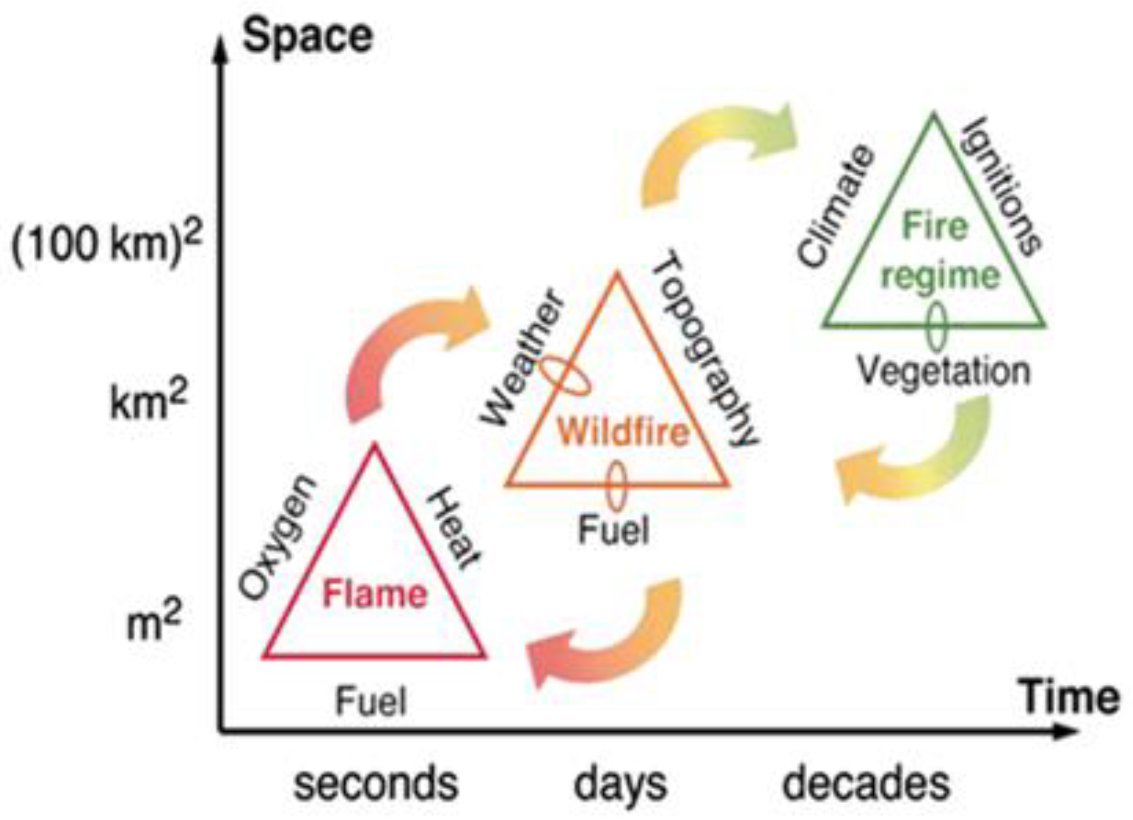
However, a more general analysis of the problem, which also includes the development of fire management plans, needs a more extended conceptual model, from fire triangle to larger scales of space and time [32]. In Figure 2, the small loops in the wildfire triangle illustrate the strong feedback between fire and the control parameters, and the arrows emphasize the feedbacks that act between scales. Together these factors govern the evolution of a fire regime, leading to characteristic patterns and approximate recurrence intervals for fires of different sizes, reflecting aspects of ecosystem structure at a relatively coarse resolution [33]. For this reason, most of the literature models are based on the definition of the parameters that characterize the fuel and the environmental conditions in which the fire develops.

2.1. The Rothermel’s Mathematical Model

The Rothermel mathematical model [28] was adopted in this paper to predict the rate of spread of fires in a continuous layer of fuel (vegetation) and in areas where there are small shrubs, with many stems and leaves, which are reasonably contiguous to the ground (approximately one meter). This is the case, for example, of the Etnean area.

The contribution for the spread of the fire by incandescent embers that can detach in anticipation of the actual fire front is neglected. This may seem like a serious limitation to the model because all people assigned to extinguish the fire know the importance of “spotting”. However, seeing the burning embers land in front of the fire front does not mean that they are crucial to the progress of the fire [33]. Moreover, we preferred here focusing on the influence of complex topographies and wind direction in the spread of fire front, rather than the ignition from incandescent embers.

The Rothermel model was developed by applying the conservation of the energy principle to a unit volume of homogeneous fuel before the advance of the fire. The speed of propagation of the fire front (in m/min) can be thus estimated as:

$$R=\frac{I_{\mathrm{R}}\xi \left(1+{\varphi }_w+{\varphi }_s\right)}{{\rho }_b\epsilon Q_{ig}},$$

(1)

where I_R is the intensity of reaction (B.t.u./ft² min), ξ is the heat flow propagation coefficient, Φ_w is the wind factor, Φ_S is the declivity factor, ${\rho }_b$ is the fuel concentration (lb/ft³), ε is the preheating index and Q_ig is the pre-ignition heat (B.t.u./lb). Thus, the numerator represents the quantity of heat received by the combustible material, while the denominator indicates the quantity of heat necessary to bring it to the ignition temperature. All input parameters can be determined from knowledge of the characteristics of the fuels in the field.

The parameters used in the definition of the fire propagation speed are shown in

Table 1. Input parameters for the Rothermel model.

Fuel Types	Symbol	Unit of Measure
Oven-dry fuel loading	W0	lb/ft2
Fuel depth	δ	Ft
Fuel particle Surface Area to Volume Ratio (SAVR)	σ	1/ft
Fuel particle low heat content	h	B.t.u./lb
Oven-dry particle density	ρp	lb/ft3
Fuel particle moisture content	Mf	-
Moisture content of extinction	Mx	-
Fuel particle total mineral content	St	-
Fuel particle effective mineral content	Se	-
Wind velocity at midflame height	U	ft/min
Slope, vertical rise/horizontal distance	ϕ	%

. Using these parameters as input to the Rothermel model, the output parameters listed in

Table 2. Output parameters for the Rothermel model.

Description	Symbol	Unit of Measure	Equation or Value
Reaction Intensity	IR	B.t.u./ ft2*min	IR = Г’wn h ηM ηS
Optimum reaction velocity	Г’	min−1	Г’ = Г’max (β/βop) A exp [A (1 − β/βop)]
Maximum reaction velocity	Г’max	min−1	Г’max= σ1.5(495 +0.0594σ1.5)−1
Optimum packing ratio	βop	-	βop = 3.348σ−0.8189
Coefficient	A	-	A = 1/(4.774σ0.1 − 7.27)
Moisture damping coefficient	ηM	-	ηM = 1 − 2.59(Mf/Mx) + 5.11(Mf/Mx)2 − 3.52(Mf/Mx)3
Mineral damping coefficient	ηS	-	ηS = 0.174Se−0.19
Propagating flux ratio	ξ	-	ξ = (192 + 0.259σ)−1exp [(0.792 + 0.681σ0.5)(β + 0.1)]
Wind coefficient	Φw	-	Φw = CUB (β/βop)−E
Coefficient	C	-	C = 7.47exp(−0.133σ0.55)
Coefficient	B	-	B = 0.02526σ0.54
Coefficient	E	-	E= 0.715 exp(−3.59 × 10−4σ)
Net fuel loading	Wn	lb/ft2	Wn = W0/(1 + ST)
Slope factor	ΦS	-	ΦS = 5.275β−0.3(tanΦ)2
Oven-dry bulk density	ρb	lb/ft3	ρb = W0/δ
Effective heating number	ε	-	ε = exp(−138/σ)
Heat of preignition	Qig	B.t.u./lb	Qig = 250 + 1116Mf
Packing ratio	β	-	Β = ρb/ρp

were obtained.

An important aspect of the Rothermel mathematical model is the definition of the characteristics of the fuels used as input parameter. Rothermel formulated eleven different “fuel models”, whose specific input parameters are reported in

Table 3. Input parameters specific for the eleven fuel models defined by Rothermel.

Fuel Types	Dead Fuel						Living Fuel		Fuel Depth
	σ	W0	σ	W0	σ	W0	σ	W0
	ft−1	lb/ft2	ft−1	lb/ft2	ft−1	lb/ft2	ft−1	lb/ft2	ft
Grass (short)	3500	0.034	- -	- -	- -	- -	- -	- -	1.0
Grass (tall)	1500	0.138	- -	- -	- -	- -	- -	- -	2.5
Brush	2000	0.046	109	0.023	- -	- -	1500	0.092	2.0
Chaparral	2000	0.230	109	0.184	30	0.092	1500	0.230	6.0
Timber (grass and understory)	3000	0.092	109	0.046	30	0.023	1500	0.023	1.5
Timber (litter)	2000	0.069	109	0.046	30	0.115	- -	- -	0.2
Timber (litter and understory)	2000	0.138	109	0.092	30	0.230	1500	0.092	1.0
Hardwood	2500	0.134	109	0.019	30	0.007	- -	- -	0.2
Logging slash (light)	1500	0.069	109	0.207	30	0.253	- -	- -	1.0
Logging slash (medium)	1500	0.184	109	0.644	30	0.759	- -	- -	2.3
Logging slash (heavy)	1500	0.322	109	1.058	30	1.288	- -	- -	3.0

.

The parameters common to all fuel models are:

• The fuel particle total mineral content, S_t = 0.0555;
• The fuel particle effective mineral content, S_e = 0.010;
• The fuel particle low heat content, h = 8000 B.t.u./lb;
• The Oven-dry particle density, ρp = 32 lb/ft³;
• The moisture content of extinction, M_x = 0.30.

The main limitations of the Rothermel model include the spread of the fire at different slopes, the wind direction and the wind intensity. For example, the model neglects the spread of a fire on a sloping ground (negative slope). In a precautionary, but untruthful way, it assumes always positive slopes, leading to conservative results, while being not very representative of the reality and therefore effective in emergency management operations. For this reason, the Rothermel mathematical model has been extended by Albini for the case of wind blowing up a slope from any angle [28,34].

For the upward diffusion with a direction concordant with wind one (upslope headfire), the Albini method reproduces the original Rothermel model. Special cases concern the remaining combinations, obtaining the complete following equations:

• Upslope Headfire:

  $$\mathrm{R}={\mathrm{R}}_0\left(1+{\mathsf{\varphi }}_{\mathrm{S}}+{\mathsf{\varphi }}_{\mathrm{W}}\right)$$

  (2)
• Downslope Headfire:

  $$\mathrm{R}={\mathrm{R}}_0\left(1+\max \left(0,{\mathsf{\varphi }}_{\mathrm{W}}-{\mathsf{\varphi }}_{\mathrm{S}}\right)\right)$$

  (3)
• Upslope Backfire:

  $$\mathrm{R}={\mathrm{R}}_0\left(1+\max \left(0,{\mathsf{\varphi }}_{\mathrm{S}}-{\mathsf{\varphi }}_{\mathrm{W}}\right)\right).$$

  (4)
• Downslope Backfire:

  $$\mathrm{R}={\mathrm{R}}_0$$

  (5)

  where R₀, ϕ_S e ϕ_W are calculated using the equations available in Table 2. Thus, the correct relation for the calculation of the fire spreading speed can be chosen taking into account only the wind direction. In fact, once set a wind direction, the conditions of headfire and backfire are automatically created, having the fire ignition point as their break. In addition, the wind direction also fixes the slope:
• The slope will be positive if in the same wind direction the altitude increases in the direction concordant with the wind;
• The slope will be negative if in the same wind direction the altitude decreases in the direction concordant with the wind.

Therefore the slope is a function of the wind direction and must be calculated from time to time.

2.2. The GIS Platform

The GIS technology represents a valid tool for applying the Albini model, since it allows to quickly produce geo-referenced raster cartography relating to the slope of the ground starting from a Digital Elevation Model (DEM) and then to simulate the propagation of a fire front in a reproducible way. The GIS implementation of the Rothermel mathematical model, with the changes made by Albini, needs the definition of the wooded area and a fire ignition point. Then, it is necessary to characterize the fuels present (i.e., the type of vegetation present).

The types of fuel identified, which represent the input parameters of the mathematical model, typically can be derived from four different methods: field reconnaissance, direct mapping methods, indirect mapping methods, and gradient modeling. Satellite remote-sensing techniques provide an alternative source of obtaining fuel data quickly, since they provide comprehensive spatial coverage and enough temporal resolution to update fuel maps in a more efficient and timely manner than traditional methods (e.g., aerial photography or recognition in the field) [35]; however, being careful that satellite signals in forested areas may be obscured by tree canopy and lead to unreliable boundaries.

The DEM should be loaded as raster geometry in the GIS environment with a very high geometric resolution (few meters, if possible). Indeed, the speed of fire spread is positively correlated with the temperature and wind force, while there is a negative correlation with relative humidity [35]. We assume a typical spreading speed, which is a few meters per second and a few orders of magnitude lower, if the fire spreads downhill and upwind. This implies the need to use a DEM whose geometric resolution is consistent with the expected advancement in order to obtain simulations as reliable as possible.

Here we give special importance to the structuring of information in order to favor the insertion and updating of all relevant data. Indeed the direct management of data in the GIS software can lead to anomalies within the database, as data redundancy and inconsistency, problems of competition for data access by multiple simultaneous users, loss of data integrity, security problems, and problems of efficiency from the point of view of data search and updating. For this reason, we designed and implemented a Relational Database Management System (RDBMS) external to the GIS platform which manages the spatial database containing the data used in the GIS application [26].

The hardware and software architecture was designed to optimize the computing resources and use of the output product. To this end, it was designed using two different hardware architectures for the spatial RDBMS and for the GIS platform: The web server is in the same machine where the RDBMS and the spatial database are located, while all GIS applications (Desktop and Web) are in the external PC. The software consists of the Desktop GIS GRASS version 7.8 and QGIS version 3.10, and PostgreSQL with the spatial PostGIS as RDBMS. Using this architecture, all the characteristics of the RDBMS and the spatial database are exploited, and the speed for updating the database modification and query is improved, thanks to a totally dedicated machine.

Our architecture is based on Geoserver (version 2.11) connected to a spatial database through to an Apache server, allowing to continuously update the database, thus optimizing the process of calculation and the generation of fire fronts as both the type of fuel and the ignition point vary [26]. The Desktop and Web GIS, as well as the database, are connected to Geoserver. In this way, updated data are always available both for simulations and for the use of output maps, to the calculation process. Using this architecture, it is possible to take advantage of the web application to set the fire ignition point in real time thanks to any detection systems present in the wooded area of interest.

2.3. Implementation of the Rothermel Model in the GIS

The Rothermel mathematical model is implemented in the GIS desktop environment following the steps described below:

• Characterization of fuel models. Recognition of fuel can take place in different ways (e.g., in the field, using existing databases of the tree species present in the area of interest, or by remote sensing);
• Choice of input parameters for the Rothermel mathematical model. The input parameters for the model are chosen for each type of fuel (among those listed in Table 3);
• Choice of output parameters for the Rothermel mathematical model. Calculation of the output parameters according to Table 2;
• Creation of vector themes, in a GIS desktop, related to the type of fuel. A shapefile is created (using the QGIS command Layer → Create vector → New shapefile), containing as many elements as the types of fuels present in the area of interest. The associated database will contain the parameters R₀, Φ_w and β;
• Rasterization of the previously created vector thematism. The shapefile is rasterized (using the QGIS command Raster → Conversion → Rasterize), generating three different raster layers in which every pixel contains the values of the parameters R₀, Φ_w and β;
• Calculation of the slope coefficient. The slope coefficient is calculated considering that for the diffusion of the fire front upwards with a direction concordant with that of the wind (upslope headfire), the Albini method uses the original Rothermel model, while for the remaining combinations, Equations (2) to (5) are used. The slope of the terrain is calculated from a DEM raster map (using the “r.mapcal” tool in the GRASS GIS), while the slope P is calculated as the ratio between the height difference of adjacent cells (depending on the wind direction) and their distance. Finally a conversion from decimal to degrees is performed, as required in the calculation of the slope coefficient ϕW (Table 2).
• Calculation of the diffusion speed of the fire front. Once R₀, Φ_w and β are estimated, the fire front diffusion speed is calculated in the presence of wind and sloping land. To do this, four zones must be distinguished: Upslope Headfire, Downslope Headfire, Upslope Backfire and Downslope Backfire (Figure 3).
  The fire ignition point is a vector thematism with punctual geometry characterized by an attribute containing the altitude value. Subsequently, taking into account the wind direction, the cartographic representation of the area of interest is divided into Backfire and Headfire, creating two elements of a polygonal vector layer. In the “Backfire” zone, the fire front spreads against the wind, while in the “Headfire” zone the fire front spreads in the direction of the wind. In the attribute table, a weight of −1 is assigned to the windward zone and 1 to the zone in the wind direction. The vector layer was then rasterized, obtaining a raster that serves as a “mask”, where −1 represents the upwind area and 1 the area in favor of the wind. Finally, considering Figure 3, the speed of the fire front in the backfire zone is determined with the following syntax:

  if (slope > 0 && DEM < height of the trigger point && mask = −1,

  R₀, R₀ (1 + max (0, ϕ_W + ϕ_S)))
  Thanks to the sign assigned to the slope coefficient, the same syntax can be used to calculate the propagation speed of the fire front in the three scenarios: “Downslope Backfire”, “Upslope Headfire” and “Downslope Headfire”, while for the “Upslope Backfire” zone, the syntax is:

  if (slope < 0 && “mask” = −1, R₀ (1 + max (0, −ϕ_S −ϕ_W)),

  Speed of the front of fire calculated in the first step)
  In this way, the diffusion speed of the fire front can be calculated for all possible cases of the Albini model, respecting the real propagation conditions.
• Representation of progress times of the fire front. A raster grid is created by associating the inverse of the speeds previously calculated in meters per second (m/s). Then, the raster GRID and the selection of the fire ignition point are used as input data to the “r.cost” GRASS GIS command. The output is a new raster layer in which the value of each cell represents the time (in seconds) required for each cell to be reached by the fire front generated by the fire ignition point (i.e., a geo-referenced cartographic representation relating to the distance traveled by the fire front after a certain time).

3. Results

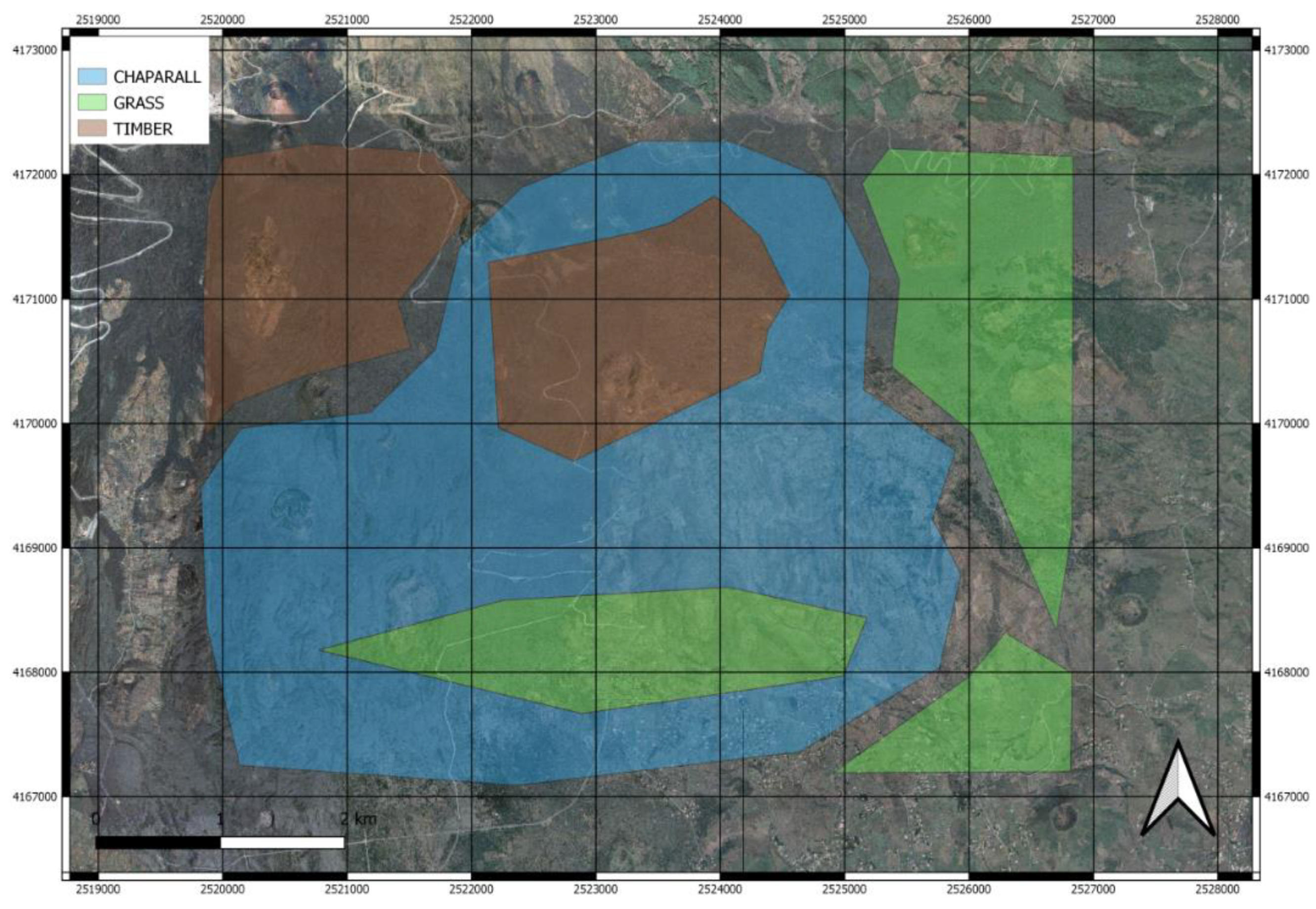
The system was tested in a wooded area on the eastern side of Mount Etna in Sicily. The area under study measures about 24.5 km² and extends for about 5.7 km in length and 4.3 km in width. This area is characterized by three different types of fuels determined through field reconnaissance: timber, chaparral and grass. Therefore a vector theme was created with polygonal geometry containing three polygons relating to the three types of fuel present in the area (Figure 4).

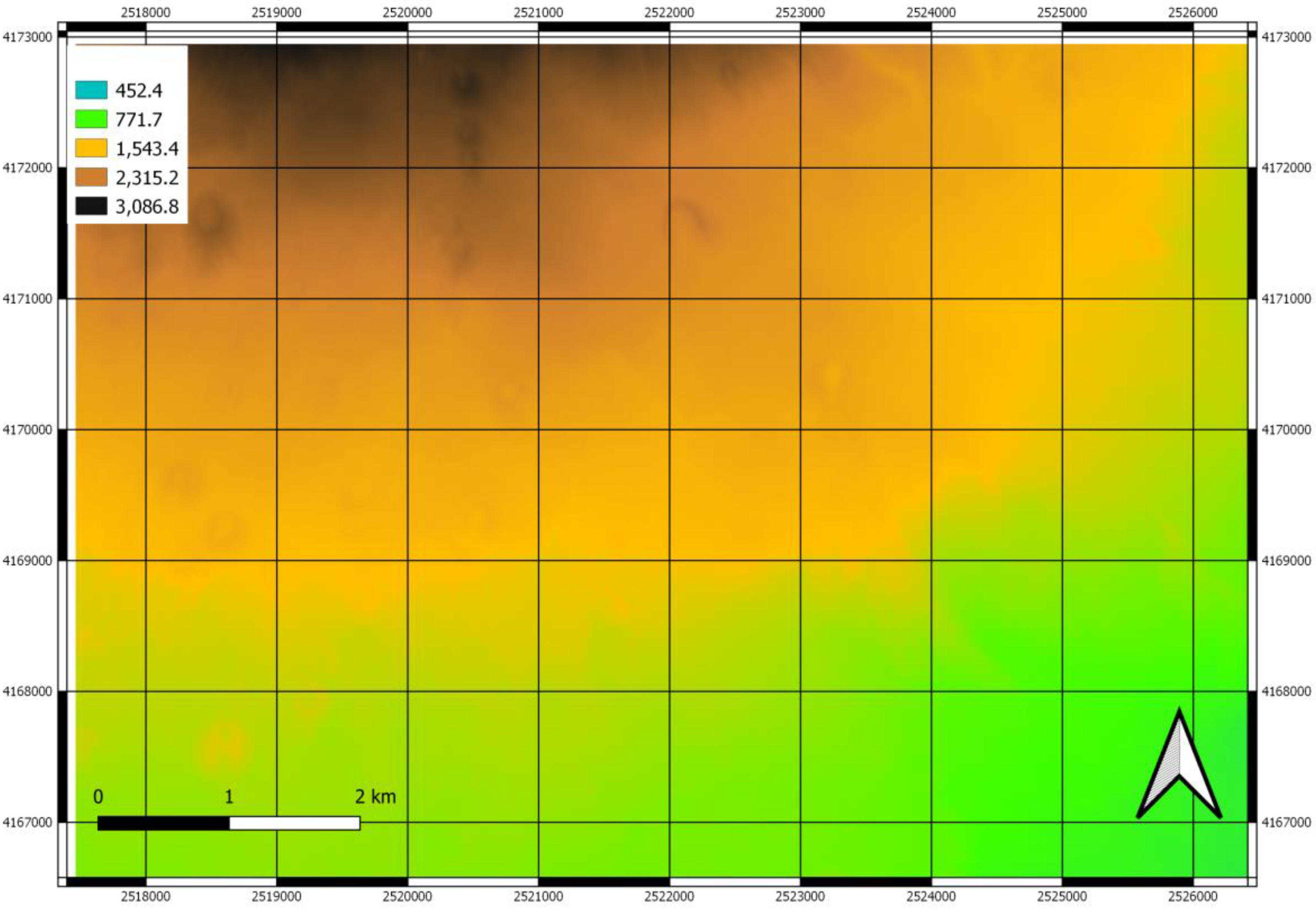
The raster DEM of the study area (Figure 5) was derived from LIDAR data acquired in 2007–2008. It was provided by the Sicily region through its cartographic portal (http://www.sitr.regione.sicilia.it/) in Gauss-Boaga reference system and a geometric resolution of 2 m.

The parameters that characterize the three types of fuel present in the study area were selected from Table 3, obtaining the values listed in

Table 4. Fuel parameters for the timber.

Parameters	Symbol	Unit of Measure	Value
Oven-dry fuel loading	W0	lb/ft2	0.138
Fuel depth	δ	ft	1
Surface Area to Volume Ratio	σ	1/ft	2000
Fuel particle low heat content	h	B.t.u./lb	8000
Oven-dry particle density	ρp	lb/ft3	25
Fuel particle moisture content	Mf	-	0.15
Moisture content of extinction	Mx	-	0.30
Fuel particle total mineral content	ST	-	0.03
Fuel particle effective mineral content	Se	-	0.01
Wind velocity at midflame height	U	ft/min	200
Slope	ϕ	%	Variable

(for the timber),

Table 5. Fuel parameters for the chaparral.

Parameters	Symbol	Unit of Measure	Value
Oven-dry fuel loading	W0	lb/ft2	0.230
Fuel depth	δ	ft	6
Surface Area to Volume Ratio	σ	1/ft	2000
Fuel particle low heat content	h	B.t.u./lb	8000
Oven-dry particle density	ρp	lb/ft3	25
Fuel particle moisture content	Mf	-	0.2
Moisture content of extinction	Mx	-	0.30
Fuel particle total mineral content	ST	-	0.03
Fuel particle effective mineral content	Se	-	0.01
Wind velocity at midflame height	U	ft/min	200
Slope	ϕ	%	Variable

(for the chaparral) and

Table 6. Fuel parameters for the short grass.

Parameters	Symbol	Unit of Measure	Value
Oven-dry fuel loading	W0	lb/ft2	0.034
Fuel depth	δ	ft	1
Surface Area to Volume Ratio	σ	1/ft	3500
Fuel particle low heat content	h	B.t.u./lb	8000
Oven-dry particle density	ρp	lb/ft3	25
Fuel particle moisture content	Mf	-	0.05
Moisture content of extinction	Mx	-	0.30
Fuel particle total mineral content	ST	-	0.03
Fuel particle effective mineral content	Se	-	0.01
Wind velocity at midflame height	U	ft/min	200
Slope	ϕ	%	Variable

(for the grass).

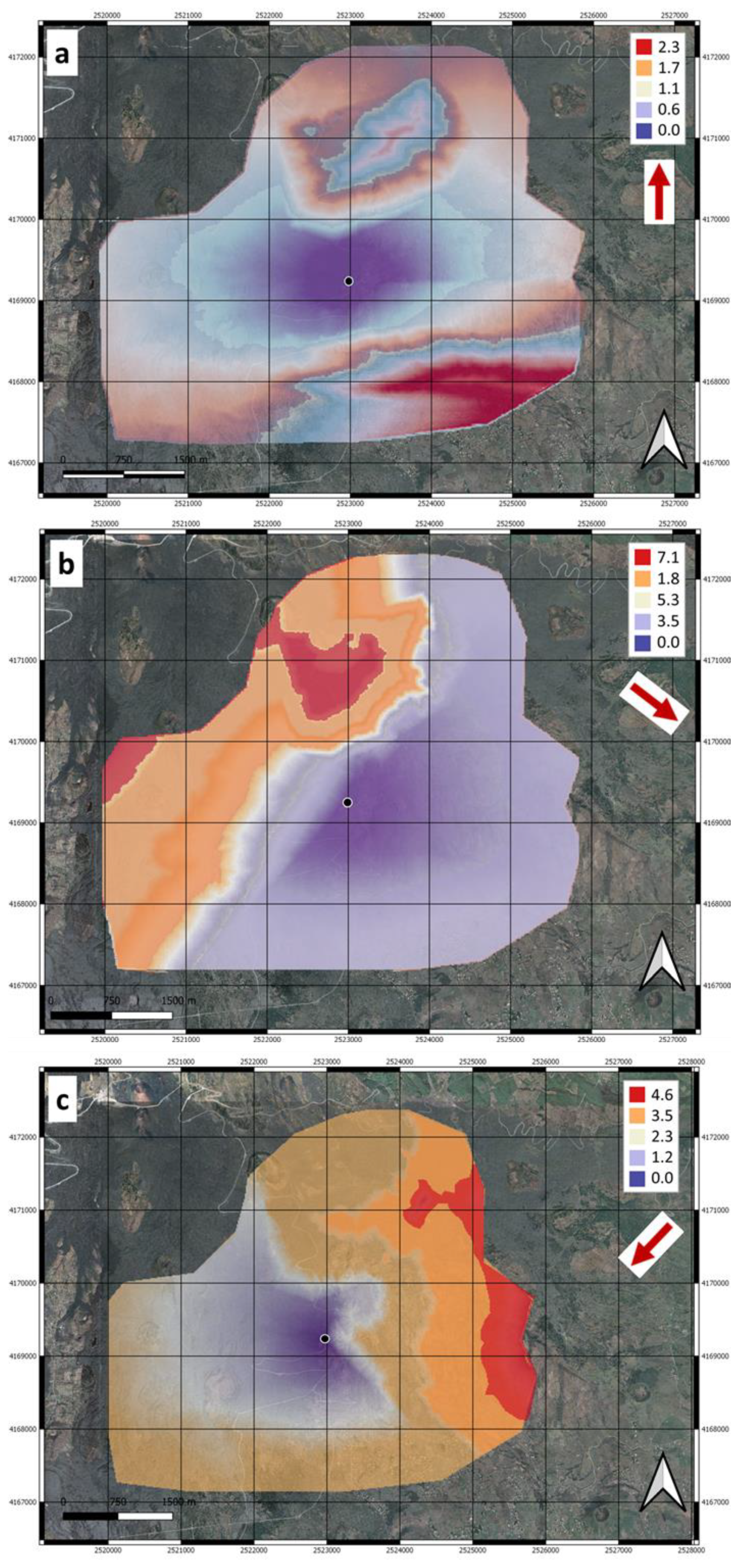
For the simulations, two different cases were hypothesized, relating to the propagation of the fire front as a function of the wind direction: The first one was carried out with a constant wind direction (Figure 6), while the second with a variable wind direction (Figure 7).

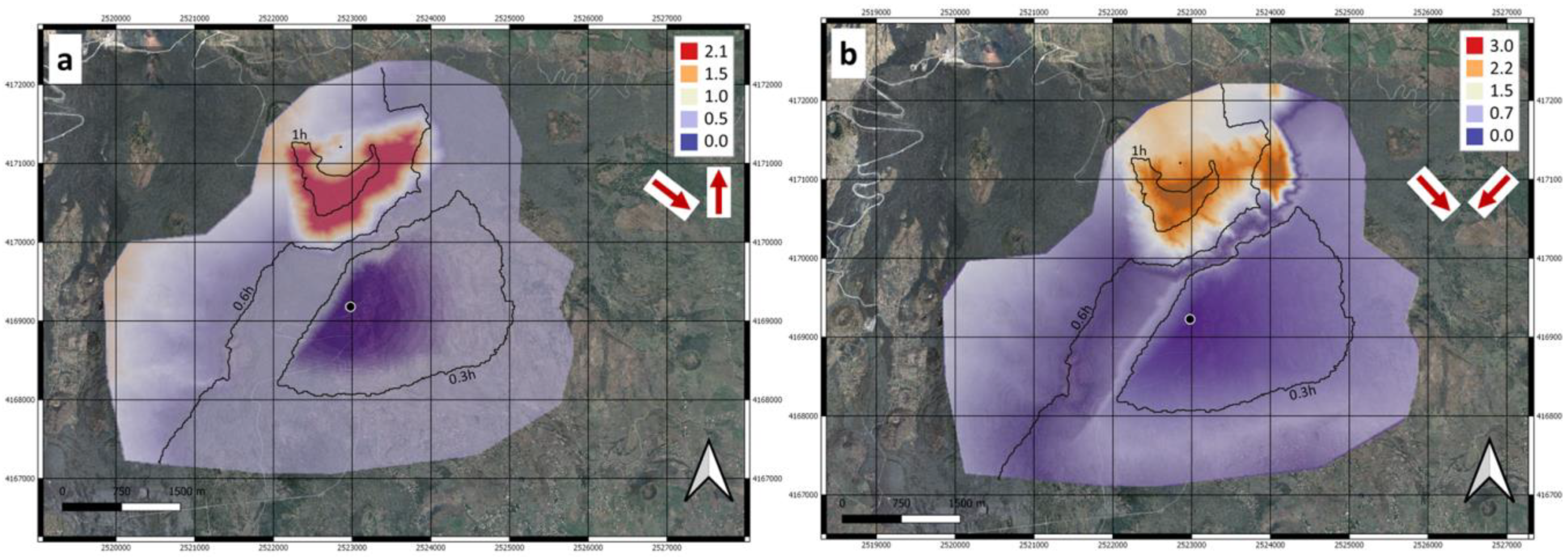
The second type of simulation was carried out considering the possibility that the wind changes direction after a certain time interval. In particular, we assumed that wind blows one hour in the South-East direction and then in the South-North direction for the first simulation (Figure 7a), and in the South-East direction and then in the South-West direction for the second simulation (Figure 7b).

4. Discussion

The Rothermel model, modified by Albini and implemented in a GIS environment, is able to simulate the propagation of a forest fire given a fire ignition point. The system allows to represent on georeferenced cartography the progress of the fire front with a reduced computational load (few minutes per simulation), making it a valuable tool for DSS in case of fire emergency.

In accordance with the Albini model, the type of fuel and the direction of the predominant wind determine the direction of advancement of the fire front. Indeed the fire spreads more easily uphill rather than downhill. Considering Figure 6, relating to the position of the fuels in the territory, it is possible to note that in the upper part of the study area, where there is litter and undergrowth, with higher humidity than the other fuels present, the fire spreads more slowly (we thus observe longer times). It is very clear in all the representations that the fire of Mediterranean scrub and grass develops more rapidly and even surrounds the area where there is litter and undergrowth. Furthermore, it can be noted that the spread of fire stops in the absence of fuel and the vegetated areas outside the ignition point are not affected by the fire.

Looking at the results shown in Figure 7, the fire front for both simulations coincides during the first hour, while the subsequent change of the wind direction determines an evident variation in the spread of the fire. This type of simulation allows to obtain in output an advancement of the fire front more similar to reality because all the points that are on the fire front at the time of the change in wind direction are considered as new ignition fire point.

Obviously, the accuracy of the results depends on the reliability of the numerical simulations and the quality of input data. These include the spatial resolution of the topography, the characterization of the fuel types and the location of the fire ignition point. However, the flexibility of the system allows updating the fire front propagation maps simply and quickly, as input parameters change. This means that any uncertainty in the input data can be corrected and new maps can be obtained by re-running the numerical simulation with the updated parameters.

5. Conclusions

With the present work, we propose a GIS application to predict and simulate the movement of the fire front in wooded areas. The application was developed by implementing the Rothermel mathematical model modified by Albini in the GIS environment in order to consider the variation of the slope and the wind direction in the propagation phases of the fire front.

The simulation results are very faithful to the real propagation of a fire front in wooded areas because in addition to the different types of fuels, we also considered the geomorphological characteristics of the territory and the environmental conditions.

The hardware and software architecture we propose is based on free and open source technologies and a relational data structure. In particular, we used the Desktop GIS GRASS and QGIS, PostgreSQL with the PostGIS extension and Geoserver. This makes possible to acquire in real time the trigger point detected by possible alert systems, to manage the output of the GIS application developed as a georeferenced raster data within the spatial database, and therefore immediately available to emergency teams.

The developed application represents an open source tool for the management of emergencies in the event of a forest fire as it allows to quickly predict the advancement of the fire front as the weather conditions change.

Future works will include, for example, the automatic detection of the fire trigger point through satellite remote sensing imagery and the extension of the GIS application by adding geospatial information, such as intervention stations, road graphs, etc., to improve its usability for civil defense purposes. In this way, by foreseeing the propagation of the fire front, it would be possible to choose an optimal path to be provided to the intervention teams in order to carry out the fire extinguishing operations in safety.

References

- Eskandari, S.; Miesel, J.R.; Pourghasemi, H.R. The temporal and spatial relationships between climatic parameters and fire occurrence in northeastern Iran. Ecol. Indic. 2020, 118, 106720. [Google Scholar] [CrossRef]
- FAO. Technical Guide for the Countries of the Mediterranean Basin. In International Handbook on Forest Fire Protection; Département Gestion Des Territoires, Division Agriculture et Forêt Méditerranéennes, Groupement d’Aix en Provence: d’Aix en Provence, France, 2000; Available online: http://www.fao.org/forestry/27221-06293a5348df37bc8b14e24472df64810.pdf (accessed on 18 June 2020).
- V T&D World Library. Wildfire Risk Mitigation for Electric Utilities. 2020. Available online: https://www.tdworld.com/wildfire/whitepaper/21125390/wildfire-risk-mitigation (accessed on 18 June 2020).
- Midgley, J.J.; Bond, W.J. Plant Adaptations to Fire: An evolutionary perspective. In Fire Phenomena and the Earth System. An Interdisciplinary Guide to Fire Science; Belcher, C.M., Ed.; Wiley-Blackwell: Hoboken, New Jersey, USA, 2013; pp. 125–134. [Google Scholar] [CrossRef]
- Bush, M.B. New and Repeating Tipping Points: The Interplay of Fire, Climate Change, and Deforestation in Neotropical Ecosystems1. Ann. Mo. Bot. Gard. 2020, 105, 393–404. [Google Scholar] [CrossRef]
- Departamento de Gestão de Áreas Públicas e de Proteção Florestal. 10.0 Relatório Provisório de Incêndios Florestais—2017; Tech. Rep.; Instituto da Conservação da Natureza e Florestas: Lisboa, Portugal, 2017; Available online: http://www2.icnf.pt/portal/florestas/dfci/Resource/doc/rel/2017/10-rel-prov-1jan-31out-2017.pdf (accessed on 18 June 2020).
- State of California. Incident Information—Numbers of Fires and Acres. Available online: http://cdfdata.fire.ca.gov/incidents/incidents_stats (accessed on 18 June 2020).
- Filkov, A.I.; Ngo, T.; Matthews, S.; Telfer, S.; Penman, T.D. Impact of Australia’s catastrophic 2019/20 bushfire season on communities and environment. Retrospective analysis and current trends. J. Saf. Sci. Resil. 2020, 1, 44–56. [Google Scholar] [CrossRef]
- San-Miguel-Ayanz, J.; Costa, H.; de Rigo, D.; Libertà, G.; Artes, T.; Durrant, T.; Nuijten, D.; Lo_er, P.; Moore, P.; Baetens, J.; et al. Basic Criteria to Assess Wildfire Risk at the Pan-European Level. 2018. Available online: https://publications.jrc.ec.europa.eu/repository/bitstream/JRC113923/jrc_tech_rep_basic_criteria_for_wildfire_risk_assessment_2018_onlinefinal_pdf.pdf (accessed on 18 June 2020).
- Finney, M.A. The challenge of quantitative risk analysis for wildland fire. For. Ecol. Manag. 2005, 211, 97–108. [Google Scholar] [CrossRef]
- Camia, A.; Houston Durrant, T.; San-Miguel-Ayanz, J. The European Fire Database: Technical Specifications and Data Submission; Publications Office of the European Union: Luxembourg, 2014; ISBN 978-92-79-35929-3. [Google Scholar] [CrossRef]
- Singh, T.; Bonne, U. Gas sensors. In Reference Module in Materials Science and Materials Engineering; Elsevier: Amsterdam, The Netherlands, 2017; ISBN 9780128035818. [Google Scholar]
- National Fire Danger Rating System. Available online: https://www.nps.gov/articles/understanding-firedanger.htm (accessed on 18 June 2020).
- Corradino, C.; Ganci, G.; Bilotta, G.; Cappello, A.; Del Negro, C.; Fortuna, L. Smart Decision Support Systems for Volcanic Applications. Energies 2019, 12, 1216. [Google Scholar] [CrossRef] [Green Version]
- Corradino, C.; Ganci, G.; Cappello, A.; Bilotta, G.; Hérault, A.; Del Negro, C. Mapping Recent Lava Flows at Mount Etna Using Multispectral Sentinel2 Images and Machine Learning Techniques. Remote Sens. 2019, 11, 1916. [Google Scholar] [CrossRef] [Green Version]
- Rogic, N.; Cappello, A.; Ganci, G.; Maturilli, A.; Rymer, H.; Blake, S.; Ferrucci, F. Spaceborne EO and a Combination of Inverse and Forward Modelling for Monitoring Lava Flow Advance. Remote Sens. 2019, 11, 3032. [Google Scholar] [CrossRef] [Green Version]
- Ganci, G.; Cappello, A.; Bilotta, G.; Del Negro, C. How the variety of satellite remote sensing data over volcanoes can assist hazard monitoring efforts: The 2011 eruption of Nabro volcano. Remote Sens. Environ. 2020, 236. [Google Scholar] [CrossRef]
- How UV, IR and Imaging Detectors Work. Available online: https://www.azosensors.com/article.aspx?ArticleID=815 (accessed on 18 June 2020).
- Famoso, D.; Mangiameli, M.; Roccaro, P.; Mussumeci, G.; Vagliasindi, F.G.A. Asbestiform fibers in the Biancavilla site of national interest (Sicily, Italy): Review of environmental data via GIS platforms. Rev. Environ. Sci. Bio Technol. 2012, 11, 417–427. [Google Scholar] [CrossRef]
- Mangiameli, M.; Mussumeci, G. Gis approach for preventive evaluation of roads loss of efficiency in hydrogeological emergencies, International Archives of the Photogrammetry. Remote Sens. Spat. Inf. Sci. ISPRS Arch. 2013. [Google Scholar] [CrossRef] [Green Version]
- Mangiameli, M.; Mussumeci, G. Real time integration of field data Into a GIS platform for the management of hydrological emergencies, International Archives of the Photogrammetry. Remote Sens. Spat. Inf. Sci. ISPRS Arch. 2013. [Google Scholar] [CrossRef] [Green Version]
- Mangiameli, M.; Mussumeci, G.; Roccaro, P.; Vagliasindi, F.G.A. Free and open-source GIS technologies for the management of woody biomass. Appl. Geomat. 2019, 11, 309–315. [Google Scholar] [CrossRef]
- Condorelli, A.; Mussumeci, A. GIS Procedure to Forecast and Manage Woodland Fires. In Geographic Information and Cartography for Risk and Crisis Management; Konecny, M., Zlatanova, S., Bandrova, T.L., Eds.; Springer: Berlin/Heidelberg, Germany, 2009. [Google Scholar]
- Nisanci, R. GIS based fire analysis and production of fire-risk maps: The Trabzon experience. Sci. Res. Essays 2010, 5, 970–977. [Google Scholar]
- Bentekhici, N.; Bella, S.; Zegrar, A. Contribution of remote sensing and GIS to mapping the fire risk of Mediterranean forest case of the forest massif of Tlemcen (North-West Algeria). Nat. Hazards 2020, 104, 811–831. [Google Scholar] [CrossRef]
- Pourghasemia, H.R.; Gayen, A.; Lasaponara, R.; Tiefenbacher, J.P. Application of learning vector quantization and different machine learning techniques to assessing forest fire influence factors and spatial modelling. Environ. Res. 2020, 184, 109321. [Google Scholar] [CrossRef] [PubMed]
- Eskandari, S.; Pourghasemi, H.R.; Tiefenbacher, J.P. Relations of land cover, topography, and climate to fire occurrence in natural regions of Iran: Applying new data mining techniques for modeling and mapping fire danger. For. Ecol. Manag. 2020, 473. [Google Scholar] [CrossRef]
- Rothermel, R.C. A Mathematical Model for Predicting Fire Spread in Wildland Fuels; USDA Forest Service; Research Paper INT-115; U.S. Department of Agriculture, Intermountain Forest and Range: Ogden, UT, USA, 1972.
- Albini, F.A. Computer-Based Models of Wildland Fire Behavior: A Users Manual; Forest Service; Intermountain Forest and Range Experiment Station, U.S. Department of Agriculture: Ogden, UT, USA, 1976.
- Zhou, X.; Mahalingam, S. Evaluation of reduced mechanism for modeling combustion of pyrolysis gas in wildland fire. Combust. Sci. Technol. 2001, 171, 39–70. [Google Scholar] [CrossRef]
- Laris, P. Integrating Land Change Science and Savanna Fire Models in West Africa. Land 2013, 4, 609–636. [Google Scholar] [CrossRef]
- Moritz, M.A.; Morais, M.E.; Summerell, L.A.; Carlson, J.M.; Doyle, J. Wildfires, complexity, and highly optimized tolerance. Proc. Natl. Acad. Sci. USA 2005, 102, 17912–17917. [Google Scholar] [CrossRef] [Green Version]
- Berlad, A.L. Fire spread in solid fuel arrays. Combust. Flame 1970, 14, 123–136. [Google Scholar] [CrossRef]
- Weise, D.R.; Bigin, G.S. A Qualitative Comparison of Fire Spread Models Incorporating Wind and Slope Effects. For. Serv. 1997, 43, 170–180. [Google Scholar]
- Tian, X.; Douglas, M.; Shu, L.; Wang, M. Fuel classification and mapping from satellite imagines. J. For. Res. 2005, 16, 311–316. [Google Scholar]
Figure 1.
The wildfire triangle conceptual model.
Figure 2.
The wildfire triangle model extended to multiple spatial and temporal scales (from [32]).
Figure 3.
Example of terrain profile with the classification of the areas according to the slope and wind direction.
Figure 4.
Orthophoto of the area under study. The vector themes with the forest types characterizing the territory are highlighted using different colors. The reference system is in Gauss-Boaga.
Figure 5.
Raster DEM of the study area. The reference system is in Gauss-Boaga; elevation in meter above sea level.
Figure 6.
Progress of the fire front (in hour) using constant wind direction. The red arrows show the direction of the wind: South-North (a), South-East (b) and South-West (c), while the central point is the fire ignition point.
Figure 7.
Propagation of the fire front advance (in hour) using variable wind directions. The red arrows show the direction of the wind: South-East and after one hour South-North (a); South-East and after one hour South-West (b). The central point is the fire ignition point. Contours represent the position of the fire front at 0.3, 0.6 and 1 h (e.g., at the time of change in wind direction).