Article

Analyzing GNSS Measurements to Detect and Predict Bridge Movements Using the Kalman Filter (KF) and Neural Network (NN) Techniques

1
Geodesy and Earth Observation Group, Department of Planning, Aalborg University, Rendsburggade 14, 9000 Aalborg, Denmark
2
School of Surveying and Geospatial Engineering, College of Engineering, University of Tehran, North Kargar Street, Central Building of the College of Engineering, Tehran 1439957131, Iran
*
Author to whom correspondence should be addressed.
Submission received: 30 December 2020 / Revised: 28 January 2021 / Accepted: 1 February 2021 / Published: 7 February 2021

Abstract

:
In this study, we present a data processing framework to apply measurements of the Global Navigation Satellite System (GNSS) technique for analyzing and predicting the movements of civil structures such as bridges. The proposed approach reduces the noise level of GNSS measurements using the Kalman Filter (KF) approach and enables the estimation of static, semi-static, and dynamic components of the bridge’s movements using a series of analyses such as the temporal filtering and the Least Squares Harmonic Estimation (LS-HE). The numerical results indicate that by using a RTK-GNSS system the semi-static component is extracted with a Standard Deviation (STD) of 0.032, 0.048, and 0.06 m in the North, East, and Up (NEU) directions, while that of the dynamic component is 0.004, 0.003, and 0.01 m, respectively. Comparing the dominant frequencies of the bridge movements from LS-HE with those of the permanent stations provides information about the bridge’s stability. To predict its deflection, the Neural Network (NN) technique is tested to simulate the time-varying components, which are then compared with the safety limits, known by its design, to assess the structural health under usual load.

1. Introduction

Nowadays, civil structures, such as bridges, have been growing ever faster to support, e.g., economical activities and attracting tourists. Long-span bridges, such as cable-stayed and suspension bridges, have been constructed to reduce their overall cost [1]. Lack of precise information on the health of their structure may lead to incorrect decision-making in repairing, retrofitting, and strengthening the structure. For example, an inadequate assessment of the structure’s health may lead to retrofit and replacement, while they are still healthy. Additionally, bridges are prone to environmental effects leading to their corrosion. Aktan et al. [2] defined Structural Health Monitoring (SHM) as the measurement of the operating and loading environment as well as the critical responses of a structure to track and evaluate the symptoms and operational incidents, anomalies, and deterioration of damage indicators, serviceability, and safety or reliability of structures. Considering their slender geometry, bridges can be affected by wind, and loads imposed by vehicles, pedestrians, etc. In addition, changes in environmental variables such as temperature might lead to changes in their deflections and corrosions, which result in changing their normal dynamic characteristics [3,4]. Therefore, it is necessary to perform health monitoring to guarantee the safety and service life of bridges, for which various techniques and methods have been proposed (see examples in [5,6]).
Generally speaking, the bridge’s movements are characterized by its static, semi-static, and dynamic components. Therefore, it is necessary to extract these components precisely to be able to model their behavior. The static component does not change over time, in other words, it shows the trend of movement, and semi-static is referred to as the long-period component. The short-period component consists of two parts: the dynamic displacements and noise, where the first changes rapidly in time and is caused by a physical process, and the latter is randomly distributed.
Among the monitoring systems, the application of the Global Navigation Satellite System (GNSS), which is weather-independent and easy to use, is ever-increasing to monitor civil structures. GNSS can be used to measure static and dynamic movement components in real-time, whereas the conventional monitoring system using accelerometers or strain gauges cannot measure static and semi-static displacements [1]. The movement estimation using geotechnical sensors such as accelerometers has their own difficulty such as their contamination with errors, e.g., drift, and the fact that they can only measure relative displacements of a structure as shown by [5,6,7]. Furthermore, the rapid advancements in GNSS devices and processing algorithms can mitigate positioning errors. In addition, integrating GNSS with supplementary sensors, such as acceleration sensors, strain gauges, and laser displacement sensors, can improve the accuracy of position estimation (see examples in [8,9]).
From various strategies of GNSS data processing, the application of the Real Time Kinematic (RTK) GNSS with a high sampling rate (>1 HZ) has already been addressed in previous studies [1,10,11,12,13]. However, the RTK system contains errors and noise of various statistical distribution (i.e., colored noise and white noise), which needs to be filtered before the precise displacement/deformation monitoring [14]. This is achieved in previous works by implementing time series analysis techniques that enable the extraction of semi-static and dynamic components.
For example, Moschas and Stiros [11] used the Moving Averaging (MA) filter to extract the semi-static movements of the Global Positioning System (GPS) measurements. Yu et al. [15] proposed a double filtration method to detect the dynamic movements of structures. Other processing techniques such as Autoregressive Integrated Moving Average (ARIMA) and Autoregressive Moving Average (ARMA) and Generalized Autoregressive Conditional Heteroskedasticity (GARCH) are investigated in [10,16,17,18,19,20,21]. Le and Nishio [21] found that the ARIMA model parameters can be used for evaluating the temporal changes of the movement components. Kaloop et al. [10] evaluated the behavior of a railway high-speed bridge and showed that the ARMA and GARCH models can be used to detect the behavior change of a bridge. Xin et al. [22] provided a new integrated method that combines the Kalman Filter (KF), ARIMA, and GARCH, where the first KF is applied on the raw position estimates to reduce the noise. Then, the ARIMA model is used to analyze and predict the structure deformation, and in the last step, the nonlinear recursive GARCH model is introduced to improve the accuracy of the prediction. Their evaluation revealed that the mean absolute error of the prediction using the KF-ARIMA-GARCH model was 10.2% less than the other time series analysis techniques. In addition to the linear models (e.g., ARMA, and ARIMA) [3,16,23,24], nonlinear models (e.g., Neural Network (NN) method, Extreme Learning Machine (ELM), and Ant Colony Optimization algorithm (ACO)) [18,25,26,27,28,29,30] have also been applied to predict the structural behaviors. These studies demonstrated that the monitoring data of huge structures (e.g., dam, bridge, and tower) contain nonlinear characteristics due to the uncertain environment [29]. As a result, the linear models represent some limitations, for example, they are only able to predict stationary (or simple non-stationary) changes. Therefore, their prediction accuracy is very limited for revealing the dynamic components.
Most of the previous studies have applied their processing approach in the time domain (see e.g., [13,14,31,32]), while only a few provided their processing steps in the frequency domain (e.g., [31,33]). The latter is performed mostly by implementing techniques such as Fast Fourier Transformation (FFT) and Wavelet Analysis, where FFT was used to estimate the natural frequency of structures and to eliminate the positioning noise, and the wavelet technique was applied to detect changes in the frequency behavior of structures [33,34,35,36,37]. However, the efficient application of FFT requires an understanding of its assumptions and limitations. For example, FFT decomposes a signal into sine and cosine functions of different frequencies. When these signals cannot be divided into the predefined cycles, amplitude-scaling errors are expected (see more details in [30]). For the RTK-GNSS derived position time series, where the signals consist of the “harmonic” and “noise” part, a more advanced methodology must be considered.
In this paper, we introduce an efficient combination of time series analysis and prediction techniques to model movements of a bridge, which is monitored by the RTK-GNSS technique. The goal is to extract the full behavior of the bridge (its static, semi-static, and dynamic components), which is achieved by applying different filtering methods. The Least Square Harmonic Estimation (LS-HE) [38] and the Neural Network (NN) [18] methods are applied to estimate the dominant frequency and to obtain the predictive movement model, respectively.
This paper is organized as follows: In Section 2, we describe the RTK GNSS-based monitoring system and characteristics of the stations used. The proposed algorithm in order to extract the bridge displacement components, as well as the displacement model are presented in Section 3. The evaluation results and numerical experiments are discussed in Section 4, which are essential for the assessment of the full behavior of the bridge, and finally, this study is concluded in Section 5.

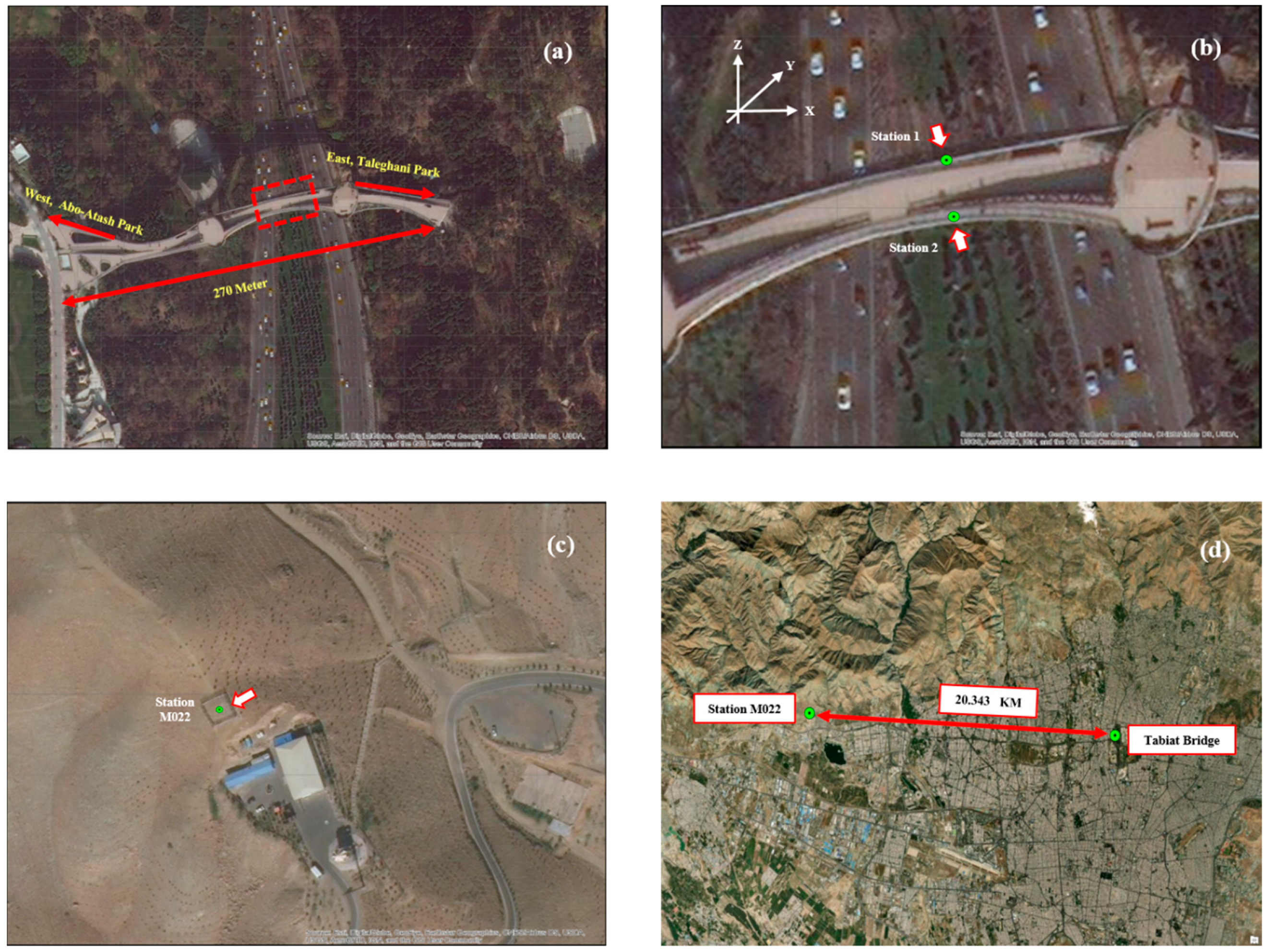
2. Tabiat Bridge and Structural Health Monitoring System Description
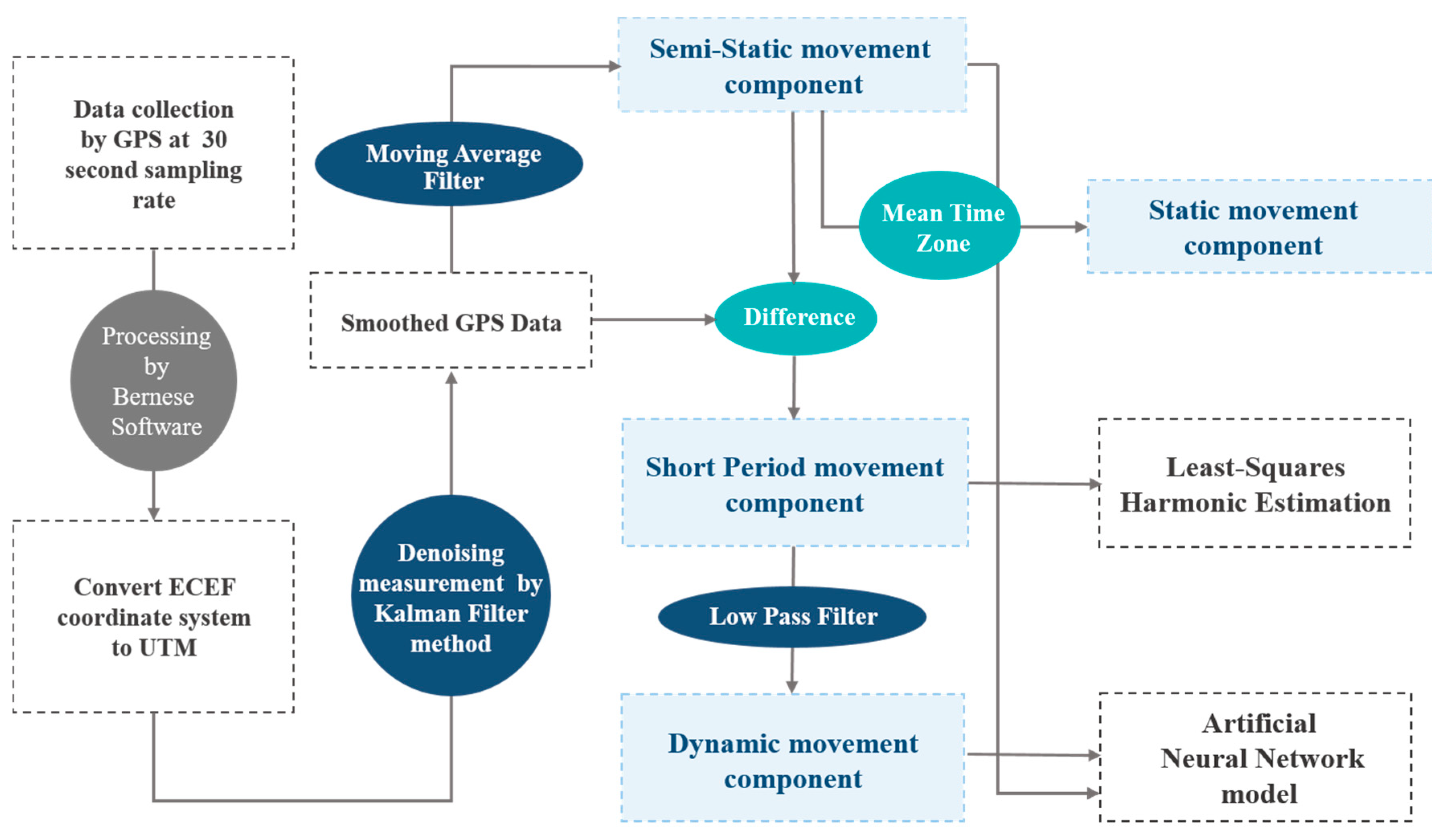
The Tabiat Bridge located in Tehran, Iran is considered as our case study. The bridge is the longest footbridge in Iran, which was opened in October 2014 to connect two public parks which are separated by a highway. As shown in Figure 1a, the total length of the bridge, which consists of four spans, (68, 94, 68, and 39 m from east to west, respectively) is about 270 m, and its width varies between 6 and 13 m. The bridge has three floors and is constructed at the height of 40 m above the (Modarres) highway. The main structure is made up of steel constitutes, but the flooring is made up of lightweight concrete and moisture insulator layers which are covered by composite wood. As shown in Figure 1b, two GNSS stations (Stations 1 and 2) are installed on this structure to measure its movements. In this study, we used one reference station of the real-time positioning system in Tehran (SAMT) to compare the movement between one permanent station and two monitoring stations along the bridge. The SAMT system consists of six reference stations for receiving data from positioning satellites. The raw GNSS measurements are used to estimate kinematic coordinates using the Bernese software (discussed in Section 4.1). As shown in Figure 1c,d, the permanent station that we used (M022) is located about 20 km from the bridge.

3. Methodology

To study the bridge’s movements, first the GNSS coordinates time-series are pre-processed using KF in order to reduce the noise [10,39,40]. A combination of the long-period (semi-static) and short-period (dynamic + noise) movement components is considered for the first try as in [39]. In Figure 2, a de-noising procedure is implemented using a Moving Average (MA) filter (with the window length of 100) [11,39] followed by the mean of semi-static movement, and a low pass filter (as the Median filter of the 20th order) to extract the semi-static, static, and dynamic components, respectively. Finally, to simulate the dynamic behavior of the bridge, the Neural Network (NN) model is used. In the following, a brief review of these techniques is presented.

3.1. Time-Series Denoising Using the Kalman Filter (KF) Approach

Taking into account the high sampling rate in the GNSS measurements and environmental factors, time-dependent variations are correlated. In addition, random errors are always present in these measurements that adversely affect the displacement analysis and may lead to undesirable results. To reduce these errors in the time-series of coordinates, as recommended, e.g., by [41], the Kalman Filter (KF) is applied to effectively reduce the random noise. In Table 1 and Table 2, the equations of KF are provided and can be divided into two groups: The time update equations and the measurement update equations [42]. The time update equations predict the current state and error covariance, to obtain the a priori estimates for the next time step. The measurement update equations are responsible for the feedback. Hence, one can interpret the time update equations as predictors and the measurement update equations as correctors.
Here, X k and X k 1 are the state vectors of the system at the time steps k and k 1 ; Φ is the state transition matrix of the dynamic model; Q x ^ k | k 1 is the estimate error covariance matrix at the time step k 1 , and Q P is the process nois.
Here, y K   is the measurement vector at the time step   K ; Q X ^ K | K is the error covariance matrix at the time step K ; A K is the design matrix which maps the true state space into the observed space; V K   is the residual (the difference between the actual and predicted measurements for the time step); R K   is the measurement error covariance matrix, and K K   is the Gain matrix at the time step k. As mentioned above, the Kalman filter uses a predictor-corrector algorithm to estimate X K , at the first step, X ^ K | K 1   is determined based on the value of X ^ K 1 | K 1 . Then, to obtain X ^ K | K , the measured value of y K is used to correct the value of X ^ K | K 1 [40,41,42,43]. In the present study, the Continuous Wiener Process Acceleration (CWPA) KF method was implemented (see the details in [43]).

3.2. Extracting the Movement Components

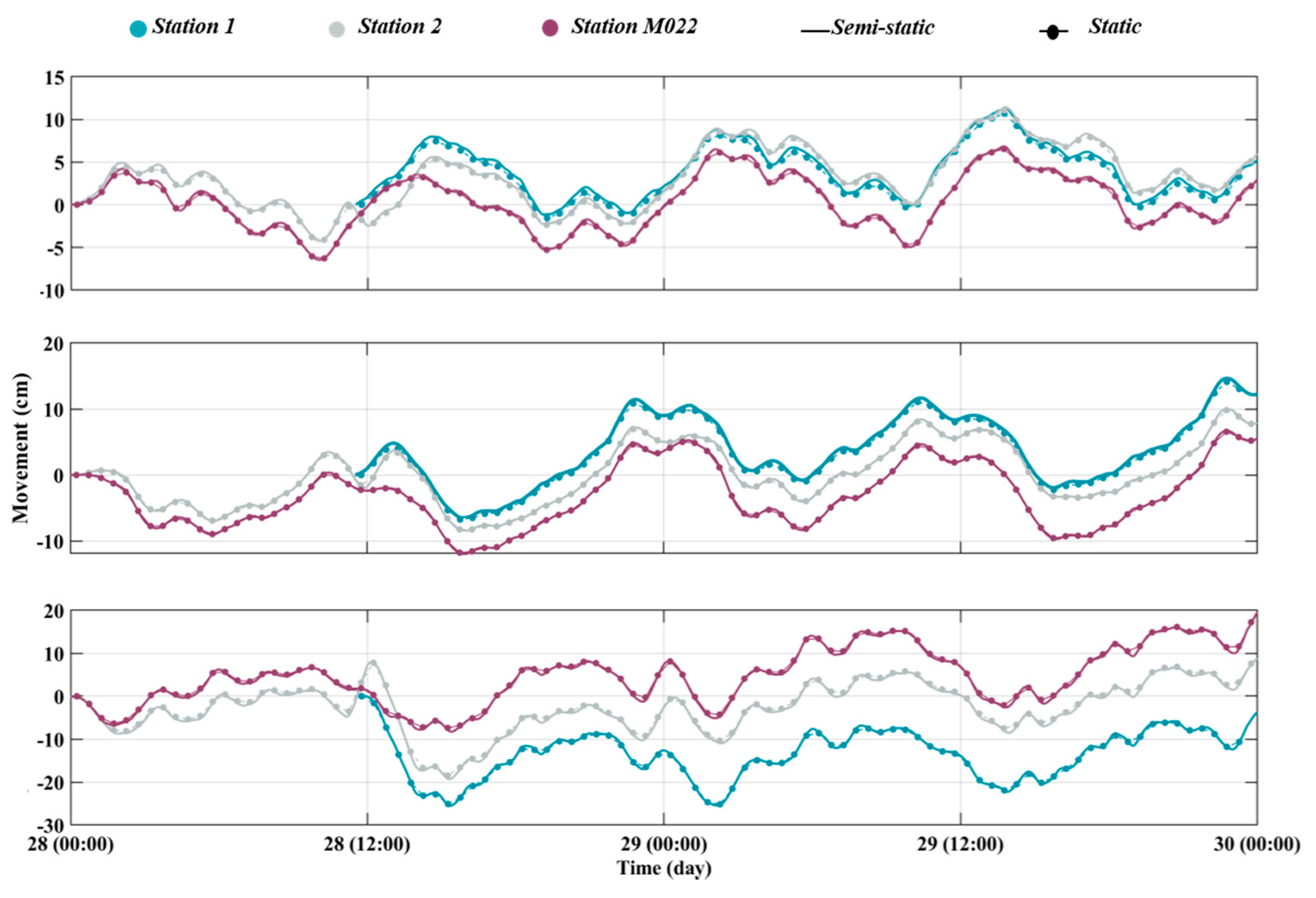
3.2.1. Semi-Static Component

The Moving Average (MA) filter has been commonly applied for smoothing short-period fluctuations and highlighting long-term trends or cycles in the time series [11,15]. However, selecting an appropriate threshold to distinguish between the short-period and long-term components depends on the application [44]. The moving average filter calculates the average of several sequential values of the input signal to produce each point of the output signal. From the mathematical point of view, the MA can be applied by convolution [44] as follows:
y [ i ] = 1 M   j = 0 M 1 x [ i + j ]
where x [] is the input signal/time-series, y [] is the output signal/time-series, and M is the number of points used in the moving average, which is selected to be M 1   h since, in this window length, the long-term component can be simulated with a high correlation to the denoised time-series. The semi-static component is extracted as long-term variations of the North, East, and Up directions.

3.2.2. Static and Short-Period Components

As shown in Figure 2, the mean of the semi-static component is used to extract the static behavior. In this study, the data sampling rate is 30 s and a mean of 5 min of the semi-static movement is considered as the static behavior of each point. The optimum number of minutes in this step is experimentally found by changing the number of minutes from 1 to 200 min. The 5 min is the one that yields the maximum similarity. The differences between the KF-smoothed time series and the static component are considered as the short-period displacements.

3.2.3. Dynamic Component

Various low pass filters such as Butterworth Filter [45], Standard Average Filter [46], Median Filter [47], and Gaussian Filter [48] are compared to isolate the dynamic component from the short-period component. To select the optimal filter, some evaluation criteria such as the Root Mean Square Error (RMSE), Mean Square Error (MSE), and Normalized Root Mean Square Error (NRMSE) are used with the formulations which are as follows:
R M S E = 1 n i = 1 n ( y i y i ) 2
M S E = y y 2 n
N R M S E = 1 y y 2 y y ¯ 2
where y represents the short-period component and y ¯ represents the reference data and the mean of vector   y , respectively; y   is the test data (dynamic component); n is the number of data, and y indicates the L2-norm of a vector y and the optimum filter can be defined by the minimum RMSE and MSE, and maximum NRMSE.

3.3. Neural Network (NN) for Prediction

The Neural Network method has been used in previous studies to determine the dynamic model of bridge movements [22,23,27,29,40]. The Multi-Layer Perceptron (MLP) network is one of the most commonly NNs, which is formed by the interconnection of some processing units known as neurons (nodes). Neurons receive information from neighboring neurons (input data) and assign weight parameters to each input. This unit is also responsible for sending the neural response of the input data using the transfer function and then sending the calculated response to the activation function of the network [49]. The MLP network consists of at least three layers: Input layer, intermediate (hidden) layer, and output layer. There is no systematic way to determine the number of hidden layers and neurons, and many factors may affect this. In this network, the input data is considered as the information of the input layer. Then, the data which are multiplied by weight factors and are added by bias, are forwarded to a hidden layer [50]. In the next step, the transform function is applied to the hidden layer information, and finally the results are considered as the input of the output layer [51]. From a mathematical point of view, neuron k can be described by Equations (5) and (6) as follows:
U k = j = 1 m W k j X j
y k = φ ( u k + b k )
where x 1 , x 2 , …, x m are inputs; w k 1 , w k 2 , …, w k m are the weights of neuron k ; and U k represents the linear combiner output of input parameters. In addition, b k is the bias; φ is the activation function; and y k is the output of the k-th neuron [50]. The input parameter is the dynamic component of the North, East, and Up, and the Neural Network predicts these components for the next 30 steps (15 min).

3.4. Least Squares Harmonic Estimation (LS-HE) Method

The Least Square Harmonic Estimation (LS-HE) is a spectral analysis technique, which is used here to compare the behavior of the stations along the bridge with the permanent station [38]. This method can improve the functional part of the observations in the frequency domain [52]. In LS-HE, the coordinates time-series are modeled as:
y = y 0 + r t + k = 1 q a k cos w k t + b k sin w k t
y = A X + k = 1 q A k X k
where Equation (8) is the matrix form of Equation (7). In both equations, the time-series y (short-period component) is modeled by fitting a linear trend and a total of q triangular terms; where t is the time; y 0 is the initial location of the station; r is the rate of linear variation of the time-series; w K is the angular velocity; and a K , b K and   k denote the unknown coefficients of cosine and sine term, and the number of frequencies, respectively. In the matrix form, A and A K are the design matrixes and X represents the vector of unknowns. In order to detect the periodic contributions, two columns of sine and cosine terms ( A K ) are added to the previous design matrix. It should be noted that adding an additional frequency must be statistically acceptable according to the following hypothesis testing:
{ H 0   : y = A X + k = 1 q 1 A k X k H a   :   y = A X + k = 1 q A k X k
where H 0 and H a   are null and alternative hypotheses, respectively. This statistical test is used repeatedly to detect different frequencies. Once each w K is accepted, the corresponding sine and cosine terms are added to the null hypothesis and the test will be performed for the subsequent frequencies. The hypothesis testing statistic at each step follows the Fisher-distribution, presented in Equation (10) as follows:
T = P ( w j ) 2 σ a 2 σ a 2 = e a T Q y 1 e a d f T F ( 2 .   m n 2 i )
where T is the test statistic; m and n are the numbers of observation and unknowns, respectively; i is the number of detected frequencies in each step; and σ a 2 is the estimated variance. In addition, w K is calculated from Equations (11)–(14) at each step as follows:
w k = a r g m a x P ( w j )
P ( w j ) = e 0 T Q y 1 A j ( A j T Q y 1 P A A j ) 1 A j T Q y 1 e 0
e 0 = P A y
P A = I A ( A T Q y 1 A ) 1 A T Q y 1
where P ( w j ) is the power spectrum, P A is the orthogonal projection matrix; Q y 1   is the inverse of the observations covariance matrix; and A is the design matrix according to Equation (15). When the statistical test of the detected frequency is confirmed, two terms of this frequency will be added to the design matrix according to Equation (16). In these equations, m denotes the number of observations.
A = [ 1 t 1 t m ]
A = [ 1 t 1 t m     c o s w k t 1 s i n w k t 1 c o s w k t m s i n w k t m ]
In practice, numerical methods such as the periodogram diagram and its visual inspection are used to extract the existing dominant frequencies, due to the complexity of these equations. A periodogram diagram presents the relation between the power spectrum and the frequency. In the next step, this diagram is used to compare the power spectrum of each frequency with its neighboring frequencies. Finally, the frequencies with a higher power spectrum will be considered as the dominant frequencies.

4. Results and Discussions

I In this section, the results of the bridge’s movement components are described, the performance of the proposed dynamic model is discussed, and the behavior of the stations along the bridge is also compared with a permanent station.

4.1. Data collection and Preparation

In this study, GNSS measurements of the Tabiat bridge (latitude: 35°45′16.15″ and longitude: 51°25′13.64″) and M022 (a permanent SAMT station, latitude: 35°45′56.97″ and longitude: 51°11′45.55″) are collected during 28–29 November 2018 with a 30 s sampling rate in order to examine the capability of the proposed algorithm. The X-direction refers to the east of the bridge (Taleghani Park), the Y-direction is perpendicular to the X-direction and is stretched along the Modares highway, and the Z-direction represents the vertical direction movement, as shown in Figure 1b. The Bernese software in a double-difference mode was utilized to process the GPS raw data of these three stations. The processing strategy is summarized in Table 3. It is worth mentioning that we used the result of the kinematic station coordinates derived from Bernese. These time-series are expressed in the local geodetic reference frame (i.e., North, East, and Up local directions). Figure 3 shows the coordinates time-series of three stations (1 fixed and 2 monitoring stations) in the Universal Transverse Mercator (UTM) grid system.

4.2. Data Pre-Processing

The KF method is used to de-noise the random errors of coordinates time-series derived from Section 4.1. The vector of coordinates time-series has an average accuracy of 0.019, 0.016 and 0.039 m during 24 h in the North, East, and Up component, respectively, which are estimated by the variance-covariance matrix of the Bernese software. After implementing the KF, the accuracy of unknown parameters reduces to 0.0013, 0.0012 and 0.0019 m in the N, E, and U directions, respectively.

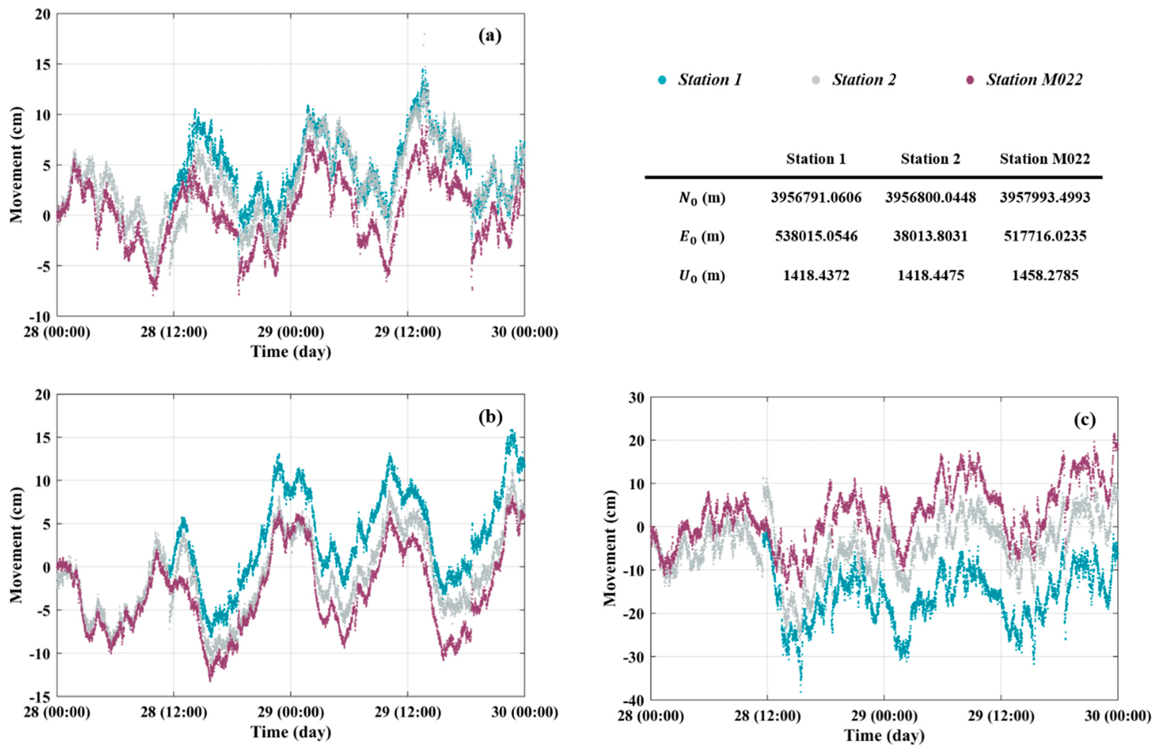
4.3. Bridge Movement Evaluation

To assess the bridge movements, the semi-static movement is considered as the first component that can be extracted by applying the MA filter to the de-noised time-series. The accuracies of semi-static components in the North, East, and Up are 0.013, 0.012, and 0.019 cm, which are determined using the least squares error propagation. Figure 4 represents the semi-static component of stations 1, 2, and M022. The results indicate that the correlation between the semi-static component and de-noised time-series is 99% at each station for the N and E components and 98% for the U component.
To assess the semi-static movement, the maximum and Standard Deviation (STD) of this component for the bridge monitoring stations are presented in Table 4. Based on Figure 4 and Table 4, the maximum movement of the stations is detected in the Up direction (0.2553 and 0.1934 m at Stations 1 and 2, respectively). Moreover, the STD value of Stations 1 and 2 in the Up direction (0.057 and 0.058 m, respectively), which is higher than in the East and North directions. The movement variations along the Up direction can be related to the load factor. In the semi-static component of the permanent station (M022), the maximum value of movement (0.1948 m) and STD (0.065 m) are found in the Up direction.
The statistical assessments provide similar results for Stations 1 and 2, which indicates that both stations have a safe semi-static behavior due to changing in the loads. Figure 5 illustrates the correlation between Stations 1 and 2, in the North, East, and Up directions. The correlation between the North and East was found to be −18.5% at Station 1 and 4.2% at Station 2. However, in Figure 5, we found that the correlation between the movements of Stations 1 and 2, in three directions is high for the same directions (e.g., the correlation between the North of Station 1 and North of Station 2 is 73.1%), which indicates that the structure movements are controlled.
As a second component, the static movement of stations is extracted using the mean of 5 min of the semi-static movement, which is also shown in Figure 4. The static behavior of Stations 1 and 2, in the East versus the North, is presented in Figure 6a, which reveals horizontal displacements. Although the static responses are found to be similar and correlated, the magnitude of this component in Station 1 is exhibited higher than those of Station 2. As Figure 6a indicates, the static response of the points is approximately similar at the end of the monitoring time, which can be associated with the negligible effect of traffic load on the bridge.
Similarly, according to Figure 6b, the static behavior of the two stations in the Up was found to be almost the same. The maximum static deviation in Station 1 (0.231 m) and Station 2 (0.167 m) occurred at time 28.59 (unit in day), which indicates the correlated behavior of two stations. Since Stations 1 and 2 are located on the left and right sides of the bridge, the situation in the location can counteract the effect of the correlated behavior. Therefore, the rigidity of the bridge structural under the traffic load effect can be concluded.
After removing the semi-static components using the MA filter from the de-noised time-series, the short-period component can be extracted which includes the dynamic component and the residual noise.
Following the description in Section 3.2.3, a low-pass filter is applied to estimate the dynamic behavior from the short-period component. In order to select the optimal filter, the evaluation criteria are evaluated, as shown in Figure 7. In this figure, it is obvious that the Median filter is the optimal method to estimate the dynamic component due to the high NRMSE and low RMSE. The dynamic behavior of the monitored points which are derived from the Median filter is presented in Figure 8.
The correlation between the dynamic components in Stations 1 and 2 are found to be 1.22%, 2.31%, and 10.28% in the North, East, and Up directions, respectively, which indicate that this component is most correlated with the Up compared to the other directions. The maximum values of dynamic movement in the Up direction are found to be 0.0464 and 0.0389 m for Stations 1 and 2, respectively. From these results, it can be concluded that the monitored points are characterized by small dynamic components, which means that the bridge is safe under the traffic loads.

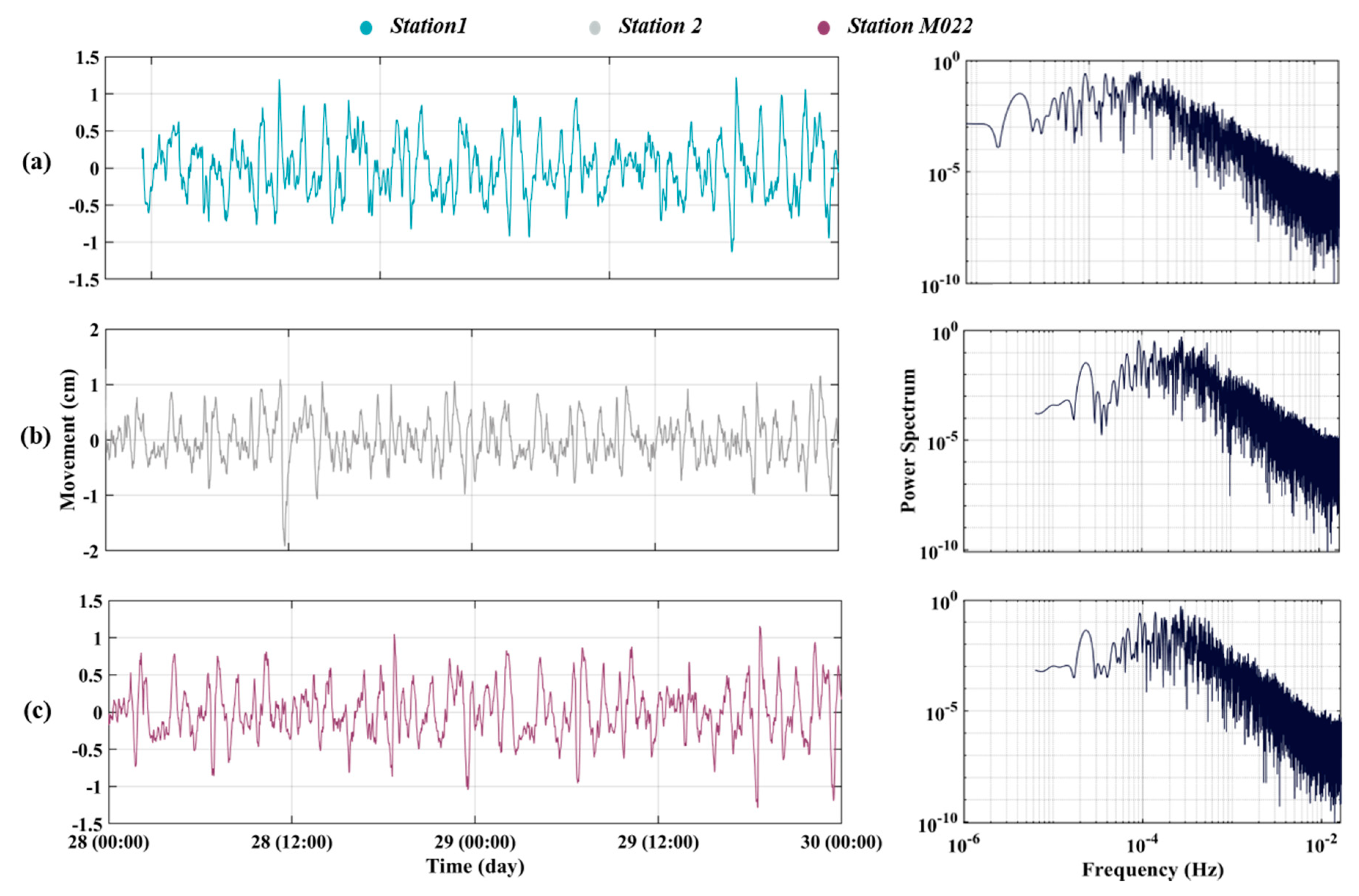
4.4. Frequency Domain Evaluation

In this section, the LS-HE method is used to evaluate the time-series response of the monitored points in the frequency domain. The short-period component is employed and LS-HE is applied to extract the dominant frequencies. The dominant frequency magnitudes for the stations along the bridge and the permanent station during the monitoring period are summarized in Table 5.
From Figure 9, it can be seen that the investigation of the short-period movement component in the time domain cannot provide any specific information. Therefore, the evaluation of this component in the frequency domain can be interesting. A comparison between the dominant frequencies derived from the three stations is shown in Figure 9, in which the log-log plot is used for the power spectrum versus frequency. Periodogram diagrams in Figure 9 and dominant frequencies values in Table 5 illustrate the similar pattern in frequencies between the station along the bridge and permanent station, which can be considered as a proof that the bridge does not show an irregular high-frequency dynamic behavior.
According to the results, we found that the mean deflections of the bridge (the mean of semi-static and short-period components) are 4.2, 3.2, and 5.2 cm in the North, East, and Up directions, respectively, and the norm of three component displacements is 7.4 cm. Therefore, the full behavior of the Tabiat bridge using GPS measurements is within the safety limits of the bridge design ([−22–22] cm).

4.5. Evaluation of the Bridge Movement Prediction Model

As mentioned in Section 3.3, the NN method is used to determine and predict the bridge movements. In the present study, a repetitive process is applied to determine the number of hidden layers and delay, and finally, the parameters with the highest level of fitting and least error was selected as the most optimal model. As a result, a neural network with five hidden layers and five delays is considered to stimulate the semi-static and dynamic components. In this study, to perform the NN method, the data set is divided into three parts randomly: Training, validation, and test data. In addition, 80%, 10%, and 10% are regarded as the training, validation, and test data set, respectively. For the semi-static component, the RMSEs between the model and the actual values in station 1 are found to be 3.78 × 10⁻⁷, 2.945 × 10⁻⁷, and 3.108 × 10⁻⁷ m in the North, East, and Up directions, while these values for Station 2 are found to be 7.623 × 10⁻⁷, 2.651 × 10⁻⁷, and 6.425 × 10⁻⁶ m. For the dynamic component, the RMSEs calculated between the model and the actual dynamic component, in Station 1, are found to be 2.478 × 10⁻⁶ m in the North direction, 1.983 × 10⁻⁶ m in the East, and 4.2 × 10⁻⁶ m in the Up direction. For Station 2, the dynamic model is fitted with 2.335 × 10⁻⁶, 2.19 × 10⁻⁶, and 3.477 × 10⁻⁶ m errors in the North, East, and Up direction, respectively. The abilities of the NN model in the prediction of semi-static and dynamic components are estimated with the RMSE values, which are summarized in Table 6. We also simulate the semi-static and dynamic components of the M022 station using this NN. The results of fitting in the prediction mode demonstrate the RMSEs of 3.894 × 10⁻⁵, 6.98 × 10⁻⁵, and 2.727 × 10⁻⁴ m in the North, East, and Up directions, respectively.

5. Conclusions

The present study evaluates the movement of a bridge using short-period monitoring by applying the RTK-GPS measurement technique. Here, we introduce a collection of signal processing techniques, which can be used for evaluating bridge movements. Our approach consists of five steps: Processing the raw GPS data, smoothing the coordinates time-series using the Kalman filter process, extracting the movement components using the moving average and median filter, determining the dominant frequencies using the least squares harmonic estimation method, and modeling the dynamic behavior by the neural network prediction technique. The concluding remarks can be summarized as follows:
  • The Kalman filter technique can be considered as a precise technique to de-noise the coordinates time-series. This method improves the uncertainty of data approximately from 0.024 to 0.0013 m.
  • The least squares harmonic estimation method was found to be efficient for extracting dominant frequencies of the dynamic component of the bridge movement, especially the step-wise statistical test avoids extracting non-meaningful dominant frequencies. The numerical results obtained from this method indicate that the bridge performance is natural under the load effect during the monitoring time.
  • Using the neural network method can be considered as an appropriate technique to forecast the dynamic and semi-static components of the bridge for 15 min. Here, the prediction model obtained an accuracy of about 6 × 10⁻⁵ and 4 × 10⁻⁵ m in the dynamic and semi-static components.
Finally, our evaluations of the static, semi-static, and dynamic behavior of the bridge indicates its safe performance under the usual loads. These findings, in the present study, can serve as a basis for an advance warning in the bridge health monitoring systems depending on the GNSS measurement technique.

Author Contributions

Conceptualization, E.F. and S.F.; methodology, E.F. and S.F.; software, K.N.; validation, K.N. and S.F.; formal analysis, E.F.; investigation, S.F. and J.P.C.; resources, E.F. and S.F.; data curation, K.N.; writing—original draft preparation, E.F., S.F., K.N. and J.P.C.; writing—review and editing, J.P.C.; visualization, S.F. and K.N.; supervision, E.F. and S.F.; project administration, S.F.; funding acquisition, E.F. and S.F. All authors have read and agreed to the published version of the manuscript.

Funding

This research received no external funding.

Institutional Review Board Statement

Not applicable.

Informed Consent Statement

Not applicable.

Acknowledgments

The authors would like to acknowledge the “Spatial Information Technology Organization” in Tehran, Iran for providing the data needed to conduct this research.

Conflicts of Interest

The authors declare no conflict of interest.

References

  1. Im, S.B.; Hurlebaus, S.; Kang, Y.-J. Summary Review of GPS Technology for Structural Health Monitoring. J. Struct. Eng. 2013, 139, 1653–1664. [Google Scholar] [CrossRef]
  2. Aktan, A.E.; Catbas, F.N.; Grimmelsman, K.A.; Pervizpour, M.; Curtis, J.M.; Shen, K.; Qin, X. Health monitoring for effective management of infrastructure. In Smart Structures and Materials Vol. 4696. 2002: SPIE: Smart Systems for Bridges, Structures and Highways, Proceedings of the SPIE’s 9th Annual International Symposium on Smart Structures and Materials, San Diego, CA, USA, 9 July 2002; International Society for Optics and Photonics: Bellingham, WA, USA, 2002. [Google Scholar]
  3. Chen, G.; Lin, X.; Yue, Q.; Liu, H. Study on separation and forecast of long term deflection based on time series analysis. J. Tongji Univ. Nat. Sci. Ed. 2016, 44, 962–968. [Google Scholar]
  4. Zhou, J.; Li, X.; Xia, R.; Yang, J.; Zhang, H. Health Monitoring and Evaluation of Long-Span Bridges Based on Sensing and Data Analysis: A Survey. Sensors 2017, 17, 603. [Google Scholar] [CrossRef] [PubMed] [Green Version]
  5. Stiros, S.C. Errors in velocities and displacements deduced from accelerographs: An approach based on the theory of error propagation. Soil Dyn. Earthq. Eng. 2008, 28, 415–420. [Google Scholar] [CrossRef]
  6. Wang, G.-Q. Some Observations on Colocated and Closely Spaced Strong Ground-Motion Records of the 1999 Chi-Chi, Taiwan, Earthquake. Bull. Seism. Soc. Am. 2003, 93, 674–693. [Google Scholar] [CrossRef] [Green Version]
  7. Yang, J.; Li, J.; Lin, G. A simple approach to integration of acceleration data for dynamic soil–structure interaction analysis. Soil Dyn. Earthq. Eng. 2006, 26, 725–734. [Google Scholar] [CrossRef]
  8. Chan, W.S.; Xu, Y.-L.; Ding, X.L.; Dai, W.J. An integrated GPS–accelerometer data processing technique for structural deformation monitoring. J. Geod. 2006, 80, 705–719. [Google Scholar] [CrossRef]
  9. Gili, J.A.; Corominas, J.; Rius, J. Using Global Positioning System techniques in landslide monitoring. Eng. Geol. 2000, 55, 167–192. [Google Scholar] [CrossRef]
  10. Kaloop, M.R.; Hu, J.W. Dynamic Performance Analysis of the Towers of a Long-Span Bridge Based on GPS Monitoring Technique. J. Sens. 2016, 2016, 1–14. [Google Scholar] [CrossRef]
  11. Moschas, F.; Stiros, S. Measurement of the dynamic displacements and of the modal frequencies of a short-span pedestrian bridge using GPS and an accelerometer. Eng. Struct. 2011, 33, 10–17. [Google Scholar] [CrossRef]
  12. Yi, T.-H.; Li, H.-N.; Gu, M. Experimental assessment of high-rate GPS receivers for deformation monitoring of bridge. Measurement 2013, 46, 420–432. [Google Scholar] [CrossRef]
  13. Yu, J.; Yan, B.; Meng, X.; Shao, X.; Ye, H. Measurement of Bridge Dynamic Responses Using Network-Based Real-Time Kinematic GNSS Technique. J. Surv. Eng. 2016, 142, 04015013. [Google Scholar] [CrossRef]
  14. Moschas, F.; Stiros, S.C. Noise characteristics of high-frequency, short-duration GPS records from analysis of identical, collocated instruments. Measurement 2013, 46, 1488–1506. [Google Scholar] [CrossRef]
  15. Yu, J.; Meng, X.; Shao, X.; Yan, B.; Yang, L. Identification of dynamic displacements and modal frequencies of a medium-span suspension bridge using multimode GNSS processing. Eng. Struct. 2014, 81, 432–443. [Google Scholar] [CrossRef]
  16. Chen, Y.; Ye, Y.-Q.; Sun, B.-N.; Lou, W.-J.; Yu, J.-H. Application of model prediction technology to bridge health monitoring. J. Zhejiang Univ. Eng. Sci. 2008, 42, 157. [Google Scholar]
  17. Chen, Z.; Zhou, J.; Tse, K.T.; Hu, G.; Li, Y.; Wang, X. Alignment control for a long span urban rail-transit cable-stayed bridge considering dynamic train loads. Sci. China Ser. E Technol. Sci. 2016, 59, 1759–1770. [Google Scholar] [CrossRef]
  18. Kao, C.-Y.; Loh, C.-H. Monitoring of long-term static deformation data of Fei-Tsui arch dam using artificial neural network-based approaches. Struct. Control. Health Monit. 2011, 20, 282–303. [Google Scholar] [CrossRef]
  19. Ossandón, S.; Bahamonde, N. On the nonlinear estimation of GARCH models using an extended Kalman filter. In Proceedings of the World Congress on Engineering, London, UK, 6–8 July 2011. [Google Scholar]
  20. Hadis Samadi, A. New GPS Time Series Analysis and a Simplified Model to Compute an Accurate Seasonal Amplitude of Tropospheric Delay. Ph.D. Thesis, The University of Western Ontario, London, ON, Canada, 2017. [Google Scholar]
  21. Van Le, H.; Nishio, M. Time-series analysis of GPS monitoring data from a long-span bridge considering the global deformation due to air temperature changes. J. Civ. Struct. Health Monit. 2015, 5, 415–425. [Google Scholar] [CrossRef]
  22. Xin, J.; Zhang, H.; Yang, S.X.; Li, X.; Wang, Y. Bridge Structure Deformation Prediction Based on GNSS Data Using Kalman-ARIMA-GARCH Model. Sensors 2018, 18, 298. [Google Scholar] [CrossRef] [PubMed] [Green Version]
  23. Cao, J.; Ding, W.-Y.; Zhao, D.-S.; Song, Z.-G.; Liu, H.-M. Time series forecast of foundation pit deformation based on LSSVM-ARMA model. Rock Soil Mech 2014, 35, 579–586. [Google Scholar]
  24. Qin, P.; Cheng, C. Prediction of Seawall Settlement Based on a Combined LS-ARIMA Model. Math. Probl. Eng. 2017, 2017, 1–7. [Google Scholar] [CrossRef]
  25. Huang, T.; Chen, X.; Liu, L. Deflection prediction of long span pre-stressed concrete beam bridgebased on ant colony optimization algorithm. J. Southeast Univ. Nat. Sci. Ed. 2013, 43, 235–240. [Google Scholar] [CrossRef]
  26. Kang, F.; Liu, J.; Li, J.; Li, S. Concrete dam deformation prediction model for health monitoring based on extreme learning machine. Struct. Control. Health Monit. 2017, 24, e1997. [Google Scholar] [CrossRef]
  27. Lai, J.; Qiu, J.; Feng, Z.; Chen, J.; Fan, H. Prediction of Soil Deformation in Tunnelling Using Artificial Neural Networks. Comput. Intell. Neurosci. 2015, 2016, 1–16. [Google Scholar] [CrossRef] [Green Version]
  28. Lian, C.; Zeng, Z.; Yao, W.; Tang, H. Ensemble of extreme learning machine for landslide displacement prediction based on time series analysis. Neural Comput. Appl. 2014, 24, 99–107. [Google Scholar] [CrossRef]
  29. Yang, J.; Zhou, Y.; Zhou, J.; Chen, Y. Prediction of Bridge Monitoring Information Chaotic Using Time Series Theory by Multi-step BP and RBF Neural Networks. Intell. Autom. Soft Comput. 2013, 19, 305–314. [Google Scholar] [CrossRef]
  30. Zhou, J.; Yang, J. Prediction of Bridge Life Based On Svm Pattern Recognition. Intell. Autom. Soft Comput. 2011, 17, 1009–1016. [Google Scholar] [CrossRef]
  31. Górski, P. Investigation of dynamic characteristics of tall industrial chimney based on GPS measurements using Random Decrement Method. Eng. Struct. 2015, 83, 30–49. [Google Scholar] [CrossRef]
  32. Yi, T.-H.; Li, H.-N.; Gu, M. Recent research and applications of GPS-based monitoring technology for high-rise structures. Struct. Control. Health Monit. 2012, 20, 649–670. [Google Scholar] [CrossRef]
  33. Larocca, A.P.C.; Schaal, R.E.; Santos, M.C.; Langley, R.B. Analyzing the dynamic behavior of suspension bridge towers using GPS. In Proceedings of the 19th International Technical Meeting of the ION Satellite Division—ION GNSS, Fort Worth, TX, USA, 26–29 September 2006. [Google Scholar]
  34. Sayed, M.A.; Kaloop, M.R.; Kim, E.; Kim, D. Assessment of acceleration responses of a railway bridge using wavelet analysis. KSCE J. Civ. Eng. 2016, 21, 1844–1853. [Google Scholar] [CrossRef]
  35. Souza, E.M.; Negri, T.T. First prospects in a new approach for structure monitoring from GPS multipath effect and wavelet spectrum. Adv. Space Res. 2017, 59, 2536–2547. [Google Scholar] [CrossRef]
  36. Taha, M.M.R.; Noureldin, A.; Lucero, J.L.; Baca, T.J. Wavelet Transform for Structural Health Monitoring: A Compendium of Uses and Features. Struct. Health Monit. 2006, 5, 267–295. [Google Scholar] [CrossRef]
  37. Yu, M.; Guo, H.; Chengwu, Z. Application of Wavelet Analysis to GPS Deformation Monitoring. In Proceedings of the 2006 IEEE/ION Position, Location, And Navigation Symposium, San Diego, CA, USA, 25–27 September 2006; pp. 670–676. [Google Scholar]
  38. Amiri-Simkooei, A.R.; Tiberius, C.C.J.M.; Teunissen, P.J.G.; Amiri-Simkooei, A. Assessment of noise in GPS coordinate time series: Methodology and results. J. Geophys. Res. Space Phys. 2007, 112, 7. [Google Scholar] [CrossRef] [Green Version]
  39. Kaloop, M.R.; Hussan, M.; Kim, D. Time-series analysis of GPS measurements for long-span bridge movements using wavelet and model prediction techniques. Adv. Space Res. 2019, 63, 3505–3521. [Google Scholar] [CrossRef]
  40. Zhang, G. Time series forecasting using a hybrid ARIMA and neural network model. Neurocomputing 2003, 50, 159–175. [Google Scholar] [CrossRef]
  41. Gul, M.; Catbas, F.N. Statistical pattern recognition for Structural Health Monitoring using time series modeling: Theory and experimental verifications. Mech. Syst. Signal Process. 2009, 23, 2192–2204. [Google Scholar] [CrossRef]
  42. Xie, Y.; Zhang, Y.; Ye, Z. Short-Term Traffic Volume Forecasting Using Kalman Filter with Discrete Wavelet Decomposition. Comput. Civ. Infrastruct. Eng. 2007, 22, 326–334. [Google Scholar] [CrossRef]
  43. Lazarov, A.; Kabakchiev, C.; Dimitrov, A.; Minchev, D. Kalman tracking filter in 3-D space. In Proceedings of the 2017 18th International Radar Symposium (IRS), Prague, Czech Republic, 28–30 June 2017. [Google Scholar]
  44. Hyndman, R.J. Moving Averages; Springer: Berlin/Heidelberg, Germany, 2011; pp. 866–869. [Google Scholar]
  45. Harvey, A.C.; Trimbur, T.M. General Model-Based Filters for Extracting Cycles and Trends in Economic Time Series. Rev. Econ. Stat. 2003, 85, 244–255. [Google Scholar] [CrossRef]
  46. Shumway, R.H.; Stoffer, D.S. An approach to time series smoothing and forecasting using the em algorithm. J. Time Ser. Anal. 1982, 3, 253–264. [Google Scholar] [CrossRef]
  47. Barner, K.E.; Arce, G.R. 21 Order-statistic filtering and smoothing of time-series: Part II. Handb. Stat. 1998, 17, 555–602. [Google Scholar] [CrossRef]
  48. Harlim, J.; Hunt, B.R. A non-Gaussian ensemble filter for assimilating infrequent noisy observations. Tellus A Dyn. Meteorol. Oceanogr. 2007, 59, 225–237. [Google Scholar] [CrossRef] [Green Version]
  49. Fröhlich, H.; Chapelle, O.; Schölkopf, B. Feature selection for support vector machines using genetic algorithms. Int. J. Artif. Intell. Tools 2004, 13, 791–800. [Google Scholar] [CrossRef]
  50. Haykin, S. Neural Networks: A Comprehensive Foundation; Prentice Hall: Upper Saddle River, NJ, USA, 1999. [Google Scholar]
  51. Davidson, R.J.; Lewis, D.A.; Alloy, L.B.; Amaral, D.G.; Bush, G.; Cohen, J.D.; Drevets, W.C.; Farah, M.J.; Kagan, J.; McClelland, J.L.; et al. Neural and behavioral substrates of mood and mood regulation. Biol. Psychiatry 2002, 52, 478–502. [Google Scholar] [CrossRef]
  52. Amiri-Simkooei, A.; Parvazi, K. Extracting tidal frequencies of the Persian Gulf and Oman Sea using multivariate least square harmonic estimation of sea level coastal height observations time series. J. Earth Space Phys. 2017, 43, 165–180. [Google Scholar]
Figure 1. (a) Tabiat Bridge plan and position (in Tehran, Iran, latitude: 35°41′47.75″ and longitude: 51°11′45.55″); (b) GNSS-based monitoring system along the bridge; (c) permanent station location; (d) distance between the monitoring and permanent stations.
Geomatics 01 00006 g001
Figure 2. The flowchart of proposed algorithm to extract different components of a bridge movement.
Geomatics 01 00006 g002
Figure 3. Coordinates time-series of three stations: (a) North; (b) East; and (c) Up components.
Geomatics 01 00006 g003
Figure 4. Semi-static and static component time-series: (a) North; (b) East; and (c) Up directions.
Geomatics 01 00006 g004
Figure 5. The correlation coefficient of the semi-static movement for the stations along the bridge. (The circles’ radius and color are associated with the numerical value of correlation).
Geomatics 01 00006 g005
Figure 6. The static components of Stations 1 and 2: (a) Horizontal displacement of the East versus North; (b) time-series in the Up direction.
Geomatics 01 00006 g006
Figure 7. Evaluation criteria of the dynamic component for Station 1: (a) North; (b) East; and (c) Up direction.
Geomatics 01 00006 g007
Figure 8. The dynamic component of the bridge’s movements: (a) North; (b) East; and (c) Up directions.
Geomatics 01 00006 g008
Figure 9. Short-period component time-series and periodogram diagram for the: (a) East of Station 1; (b) east of Station 2; and (c) east of Station M022.
Geomatics 01 00006 g009
Table 1. Kalman Filter time update equations.
X ^ K | K 1 = Φ X ^ K 1 | K 1
Q X ^ K | K 1 = Φ Q X ^ K 1 | K 1 Φ T + Q P
Table 2. Kalman Filter measurement update equations.
V K = y K A K X ^ K | K 1
K K = Q X ^ K | K 1 A K T ( A K Q X ^ K | K 1 A K T + R K ) 1
X ^ K | K = X ^ K | K 1 + K K V K
Q X ^ K | K = ( I K K A K ) Q X ^ K | K 1
Table 3. An overview of the observation, models and processing strategy used for the network of this study.
GNSS System(s)GPS Only
Basic observablecarrier phase with an elevation angle cutoff of 7° and a sampling rate of 30 s.
Modelled observableDouble differences of the ionosphere-free linear combination.
Ground antenna phase center calibrationsIGS08 absolute phase-center variation model is applied.
Tropospheric ModelA priori model is the GMF mapped with the DRY-GMF.
Tropospheric Mapping FunctionGMF
IonosphereFirst-order effect eliminated by forming the ionosphere-free linear combination of L1 and L2. Second and third effect applied.
Center orbit timefinal
Station coordinatesCoordinate constraints are applied at the Reference sites with standard deviation of 1 mm and 2 mm for horizontal and vertical components respectively.
AmbiguityAmbiguities are resolved in a baseline-by-baseline mode using the Code-Based strategy for 180–6000 km baselines, the Phase-Based L5/L3 strategy for 18–200 km baselines, the Quasi-Ionosphere-Free (QIF) strategy for 18–2000 km baselines and the Direct L1/L2 strategy for 0–20 km baselines.
Terrestrial reference frameIGS08 station around Iran (ankr, artu, drag, nico, polv, tehn, zeck) coordinates and velocities mapped to the mean epoch of observation.
Table 4. Statistical analysis of semi-static component (unit in meter).
Statistical ParameterStation 1Station 2
NEUNEU
MAX0.11330.14650.25530.11450.10010.1934
STD0.030.050.0570.0350.0450.058
Table 5. Dominant frequencies for the monitoring points (unit in Hz).
PointNEU
Station 10.000520.000280.00022
Station 20.000350.000270.00022
Station M0220.000310.000260.00024
Table 6. The assessment of semi-static and dynamic components in the prediction mode using the neural network technique (NN).
Semi-StaticDynamic
NEUNEU
RMSEStation 14.736 × 10−52.676 × 10−50.00127.940 × 10−53.490 × 10−57.807 × 10−5
Station 29.772 × 10−54.371 × 10−50.00020.00016.616 × 10−50.0002
Publisher’s Note: MDPI stays neutral with regard to jurisdictional claims in published maps and institutional affiliations.

