Application of Multimodel Superensemble Technique on the TIGGE Suite of Operational Models


1
Center for Ocean-Atmospheric Prediction Studies, Florida State University, Tallahassee, FL 32304, USA
2
Florida Climate Institute, Florida State University, Tallahassee, FL 32304, USA
3
Department of Environmental Engineering, Texas A&M University, Kingsville, TX 78363, USA
4
School of the Environment, Florida Agricultural and Mechanical University, Tallahassee, FL 32307, USA
5
National Weather Forecasting Center, India Meteorological Department, Ministry of Earth Sciences, New Delhi 110003, India
*
Author to whom correspondence should be addressed.
Geomatics 2021, 1(1), 81-91; https://0-doi-org.brum.beds.ac.uk/10.3390/geomatics1010007
Submission received: 18 December 2020
/
Revised: 10 February 2021
/
Accepted: 17 February 2021
/
Published: 19 February 2021
Abstract
:One widely recognized portal which provides numerical weather prediction forecasts is “The Observing System Research and Predictability Experiment” (THORPEX) Interactive Grand Global Ensemble (TIGGE), an initiative of WMO project. This data portal provides forecasts from 1 to 16 days (2 weeks in advance) for many variables such as rainfall, winds, geopotential height, temperature, and relative humidity. These weather forecasting centers have delivered near-real-time (with a delay of 48 hours) ensemble prediction system data to three TIGGE data archives since October 2006. This study is based on six years (2008–2013) of daily rainfall data by utilizing output from six centers, namely the European Centre for Medium-Range Weather Forecasts, the National Centre for Environmental Prediction, the Center for Weather Forecast and Climatic Studies, the China Meteorological Agency, the Canadian Meteorological Centre, and the United Kingdom Meteorological Office, and make consensus forecasts of up to 10 days lead time by utilizing the multimodal multilinear regression technique. The prediction is made over the Indian subcontinent, including the Indian Ocean. TRMM3B42 daily rainfall is used as the benchmark to construct the multimodel superensemble (SE) rainfall forecasts. Based on statistical ability ratings, the SE offers a better near-real-time forecast than any single model. On the one hand, the model from the European Centre for Medium-Range Weather Forecasting and the UK Met Office does this more reliably over the Indian domain. In a case of Indian monsoon onset, 05 June 2014, SE carries the lowest RMSE of 8.5 mm and highest correlation of 0.49 among six member models. Overall, the performance of SE remains better than any individual member model from day 1 to day 10.
1. Introduction
Prediction of day-to-day weather is becoming critical for most purposes. Many forecasting centers such as the National Centre for Environmental Prediction (NCEP), the United Kingdom Meteorological Office (UKMO), and the European Centre for Medium-Range Weather Forecasts (ECMWF) are issuing 6–7 days of forecasts with greater confidence [1,2]. Individual models’ performance is enhancing due to advanced physics for higher horizontal resolution, better quality in situ data, and the incorporation of data assimilation techniques [3]. One of the essential components of today’s prediction success goes to more data being available for data assimilation. A reliable two week forecast for rain is highly desirable for agricultural uses [4]. Most of the farmlands in India are monsoonal rain-fed for rice crops.
Furthermore, these regions are vulnerable to drought and flood events. Timely advanced information could help farmers plan appropriate seeding cultivating and other field activities, which will surely help to enhance crop production. There is a need for accurate models to forecast from daily to the medium-range time scale in this case. The accuracy of each model varies from region to region and day-to-day. Most of the weather prediction centers are engaged in improving the model’s forecast, including the model’s uncertainty, error, and need for improvements [5,6,7]. To consider better forecasting of rainfall, a statistical tool like multimodel has shown relatively better results [8,9]. Over the Indian region, single model and multimodel techniques were designed to predict and improve rainfall forecasts from the statistical postprocessing of model outputs [10]. Operational weather forecasting centers use ensemble techniques that involve several model-based ensembles as well as multimodel ensembles. These centers are the National Centre for Medium Range Weather Forecasting (NCMRWF)-India [11], NCEP-USA [12], and APEC Climate Center (APCC) South Korea [13].
Here, we implemented the multimodel superensemble (SE) technique for a set of global operational models to emphasize this technique’s strength for operational forecasts in real-time for Indian monsoon regions. The observed rainfall rate requirement for the global SE technique is fulfilled using rainfall estimates from the Tropical Rainfall Measuring Mission (TRMM). The need for member models for SE is achieved by the use of model outputs from “The Observing System Research and Predictability Experiment” (THORPEX) Interactive Grand Global Ensemble (TIGGE). One of its main objectives is to enhance collaboration in the development of ensemble prediction between operational centers and universities by increasing the availability of Ensemble Prediction System (EPS) data for research. It routinely provides real-time daily weather forecasts from ten global centers. It is a crucial component of the World Weather Watch Programme that attempts to improve the forecast skill for medium-range scales of 1 day to 2 weeks and bridges the gap between the academic and operational worlds [14]. These weather forecasting centers have delivered near-real-time (with a delay of 48 hours) EPS data to three TIGGE data archives since October 2006. Various skill matrices and performance statistics of rainfall forecast are mentioned in [15,16].
2. Datasets and Methodology
2.1. Datasets of the TIGGE Suite
We utilize the TIGGE suite of ensemble forecast data in this study. This suite consists of 10 global numerical weather prediction centers with a dataset starting from October 2006. These centers are the European Centre for Medium-Range Weather Forecasts (ECMWF), the National Centre for Environmental Prediction (NCEP), the Center for Weather Forecast and Climatic Studies (CPTEC), the China Meteorological Agency (CMA), the Canadian Meteorological Centre (CMC), the United Kingdom Meteorological Office (UKMO), the Australian Bureau of Meteorology (BOM), the France Meteorological Agency (Meteo-France), the Korea Meteorological Agency (KMA), and the Japan Meteorological Agency (JMA). We use outputs from six centers—CMA, CMC, CPTEC, ECMWF, NCEP, and UKMO—and use the SE approach to create consensus predictions of up to 10 days of lead time. The six models were selected on the basis of their consistency in runtime and the predicted availability of valid data (12 UTC). Validity time was taken to be 12 UTC to validate the totals of normal TRMM precipitation. While there is a network of observation stations in the National Meteorological and Hydrological Centers (NMHCs) worldwide, they are not dense enough. Thus, data from such stations are not necessary. TRMM, which is a joint venture between the National Aeronautics and Space Agency (NASA) and Japan Aerospace Exploration Agency (JAXA), is, therefore, a great idea as they provide high-resolution data spanning the entire globe [17,18,19,20]. TRMM3B42 daily accumulated rainfall data are used in this study, available from 01 Jan 1998 to 30 Sep 2014. The resolution of TRMM3B42 rainfall data is 0.25° × 0.25° in space. Forecast datasets from TIGGE and rain rates from TRMM (accumulated daily totals) were regridded to 25km standard resolution using bilinear interpolation method and were used to construct an SE precipitation forecast at each grid point. We have selected the above six models’ forecasts up to 10 days lead time every day at 12 UTC for Indian summer monsoon seasons June, July, August, and September (JJAS) from 2008 to 2013, the six years for this study. Based on the total number of 122 days in a JJAS season and the total of 732 cases that were present in six years (2008–2013), most cases would most likely be appropriate for depicting the features of a forecasting algorithm. This research refers only to precipitation variables that are highly stochastic in nature and, preferably, its accurate prediction involves a more complex and more detailed modeling compared to the other variables.
The majority of the numerical weather prediction centers in the world operate models that span the entire globe, and the TIGGE archive provides access to the TIGGE data after the forecast’s initial time [14,21]. The main characteristics of the six selected ensemble prediction systems tested are shown in Table 1.
2.2. Methodology
As given in [9,22], the creation of a multimodel superensemble (SE) prediction is accomplished at a given grid point by using the following expression that relates the model forecasts and observed state to SE forecast as,
where = temporal mean of observed state, k = model index, ak = coefficients for a model k, N = number of models, = temporal mean of prediction by model k during the training period, and = forecast from model k. The coefficients are computed at each grid point by minimizing the following function:
where is the observed state, t represents time, and T stands for the training period’s length. The stabilized coefficients are obtained by the least square minimization of errors from the anomaly correlation matrix obtained by substituting Equation (1) into Equation (2). The transform equation after minimization with respect to the coefficients can be represented in the form of a normal equation of the form as in Equation (3).
where we define and .
The matrix R depends only on the basis functions, and it does not involve the values of the observed data. We utilize the singular value decomposition (SVD) methodology to compute the coefficients. The SVD method removes the singular matrix problem that cannot be solved with the Gauss–Jordan elimination method [23].
We did not show the results from the ensemble mean where there were equal coefficients. Ensemble mean is the baseline criterion for any technique of assigning unequal coefficients such as SE that often performs better than ensemble mean [24].
The superensemble method makes a calculation of the coefficients by reducing collective local biases in space and time for different variables from different models. The multimodel superensemble utilizes multiple coefficients against the reduction in any systemic errors. This is computationally inexpensive and can be run in real-time in a very short period of time. There are a number of published studies on the application of SE technique which show its implementation of many other variables, regions, and hurricane real-time forecasting where this technique emerges as a more reliable postprocessing tool [24].
3. Results
3.1. Model Performances for 1–10 Days
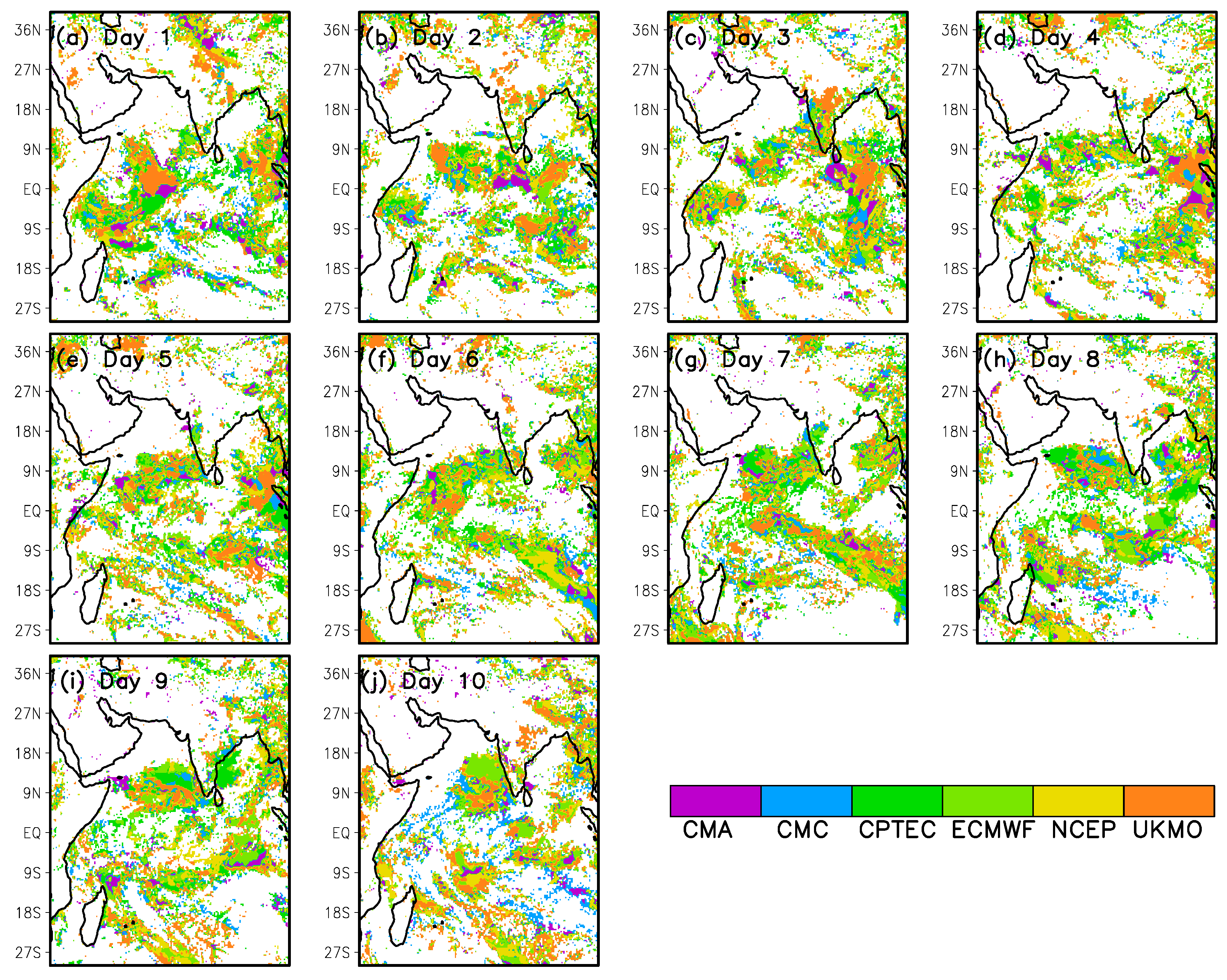
We first ask the question of how each model performs against the observation at each grid point. This information is beneficial to know for each model in identifying its regional skills. For this purpose, a sample of precipitation forecast skills in the form of absolute minimum error is illustrated in Figure 1a–j for days 1 through 10. At each grid point of the domain, model performance is evaluated. A member model, which carries the smallest absolute error among others, is represented for day 1 to 10 at that grid point of the domain. A few noteworthy observations could be made in the spatial distribution in panels (a) through (i) that the best model carrying the orange color is the UKMO model, which outperformed all operational models. Over the ocean, the UK Met Office model, NCEP, ECMWF, and CPTECH perform well for all days, but the performance of the CMA and CMC model is inferior. Another critical point drawn from the figure is that not a single model color covers the entire domain. Still, all models show their significance in terms of best absolute error locally.
This also shows that it is not wise to rely on forecasts from a single model. Extracting useful information from the worst and good operational models becomes essential and the first step towards achieving the best forecast from currently available resources. For this purpose, it is vital to extract useful information from the history of the forecast data and correcting the estimates based on that information.
3.2. Stability of Coefficients
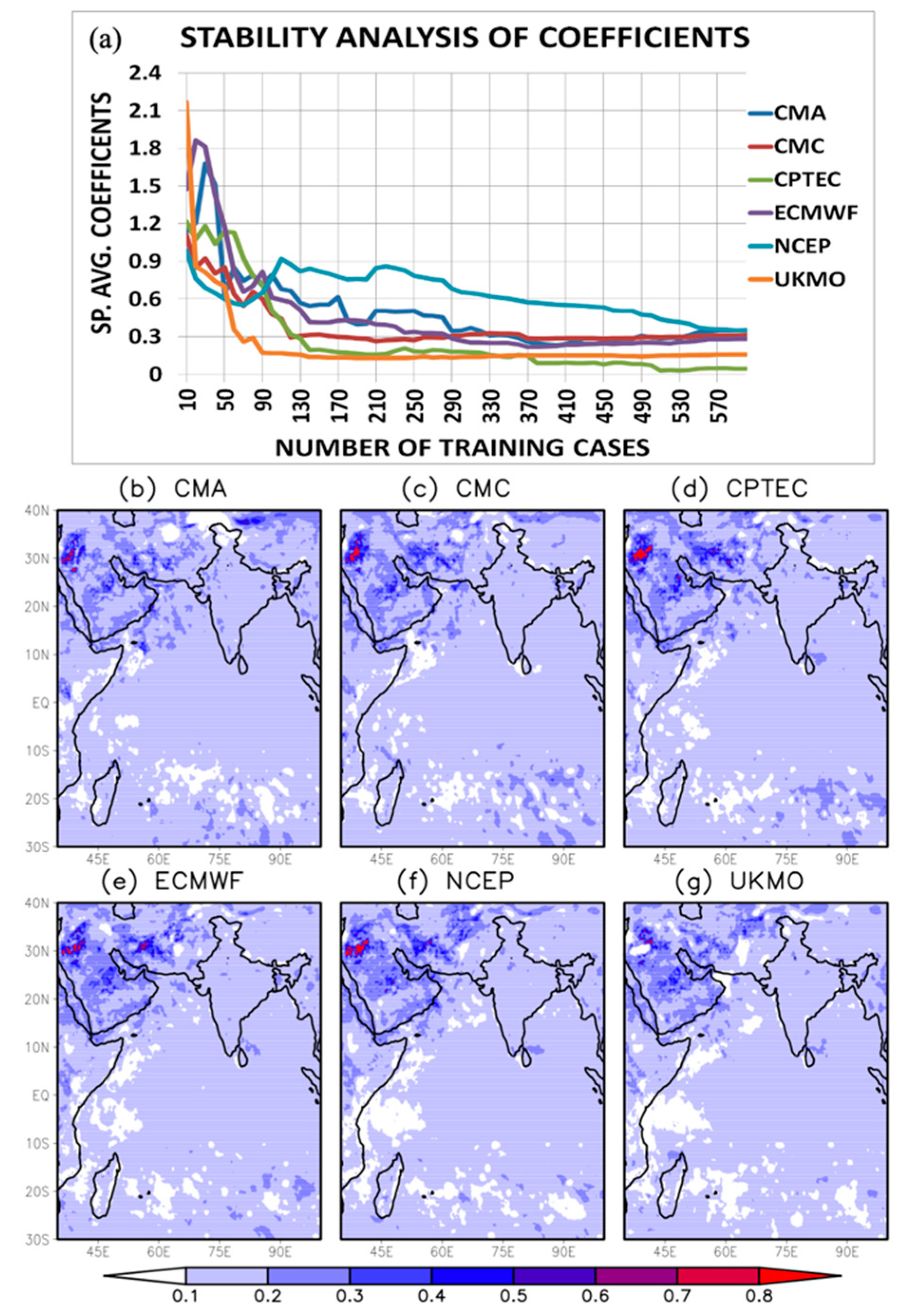
SE is one such technique based on the least square minimization of errors from the anomaly correlation matrix. It assigns the unequal coefficients to each model at each grid point based on their performance history during the training phase, which performs better than the equal coefficients base criteria [24]. In the multimodel SE technique, coefficients can be positive or negative, which is one of the benefits over ensemble mean, where coefficients are positive only. Therefore, it becomes essential to have an SE forecast, which is a single model consensus forecast based on the best available operational models. This is conducted by comparing the model forecasts with TRMM analysis fields at each grid point, having the primary objective of developing statistics based on the least square fit. It adopts a particular way of assigning coefficients to the models derived from their past performance. It awards positive, negative, and even fractional coefficients, thereby eliminating the model’s overfitting. It, therefore, evaluates model biases geographically. We carried out the regression coefficients‘ stability analysis against the training phase periods to obtain the optimal value of regression coefficients. Out of 732 days of JJAS ((30 + 31 + 31 + 30) * 6), the first 600 days were used in the training phase to calculate stable statistical coefficients. A safe selection was rendered by using the best projection that satisfies the stability criteria on the spatially averaged curve of the data in Figure 2a. While robust results can be obtained from a large number of cases, a minimum number of 90 days is also used in the training phase in the study [24], where there is a restricted number of cases available for training phases.
Figure 2a shows six member models’ (day one forecasts) domain-averaged regression coefficients. In the figure, the abscissa indicates the number of training days, which are being increased cumulatively with a step size of 10 days. The ordinate shows corresponding domain-averaged coefficients. The spatial average coefficients vary positively only in the range [0.07–2.2] for the Indian domain only, which can also be validated in the spatial distribution of coefficients shown in Figure 2b–g. There are a number of studies to find criteria from for temporal stability in regression models for a minimum number of cases. The authors in [24] claim that 90–120 days are sufficient to obtain reliable coefficients, which can also be seen in Figure 2a, in which coefficients start to become stable (parallel to abscissa). We also can see that almost all models (except CMA and NCEP) have achieved stable values after 130 training cases. All models acquire stable values after 545 days. Therefore, the use of 600 training days for this study is justified and safe. These coefficients are then passed to the forecast phase and used to construct the SE real-time forecasts for onset dates during the southwest monsoon of 2014.
3.3. Rainfall Variability from 6 Models
The onset of the southwest monsoon over Kerala signals the monsoon’s arrival over the Indian subcontinent and represents the beginning of India’s rainy season. We applied these stable coefficients to the real-time case studies with a forecast lead time of 10 days.
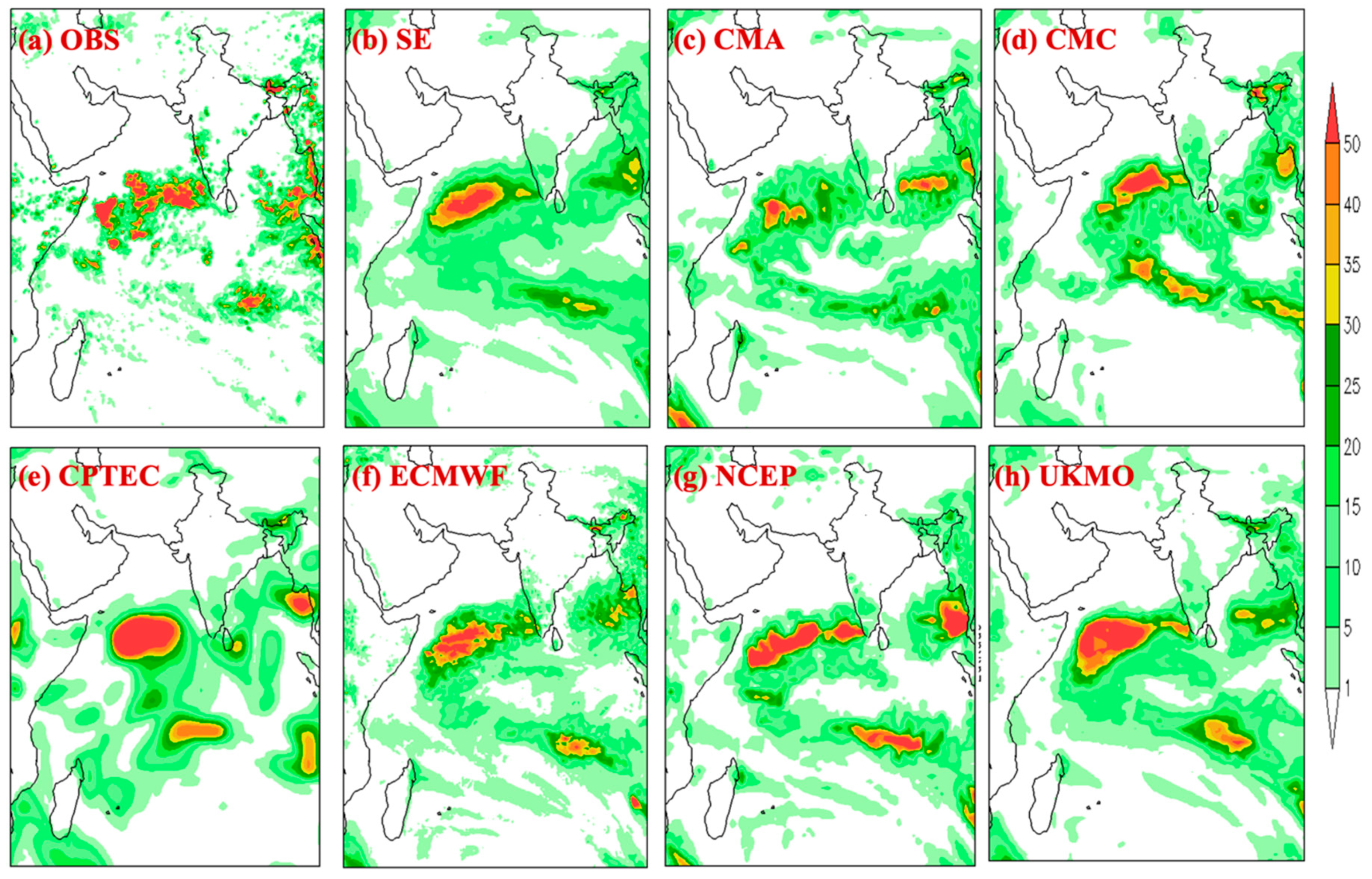
The spatial distribution of precipitation on the onset date 05 June 2014 (day one forecast only) for the observed, SE, and member models are shown in Figure 3.
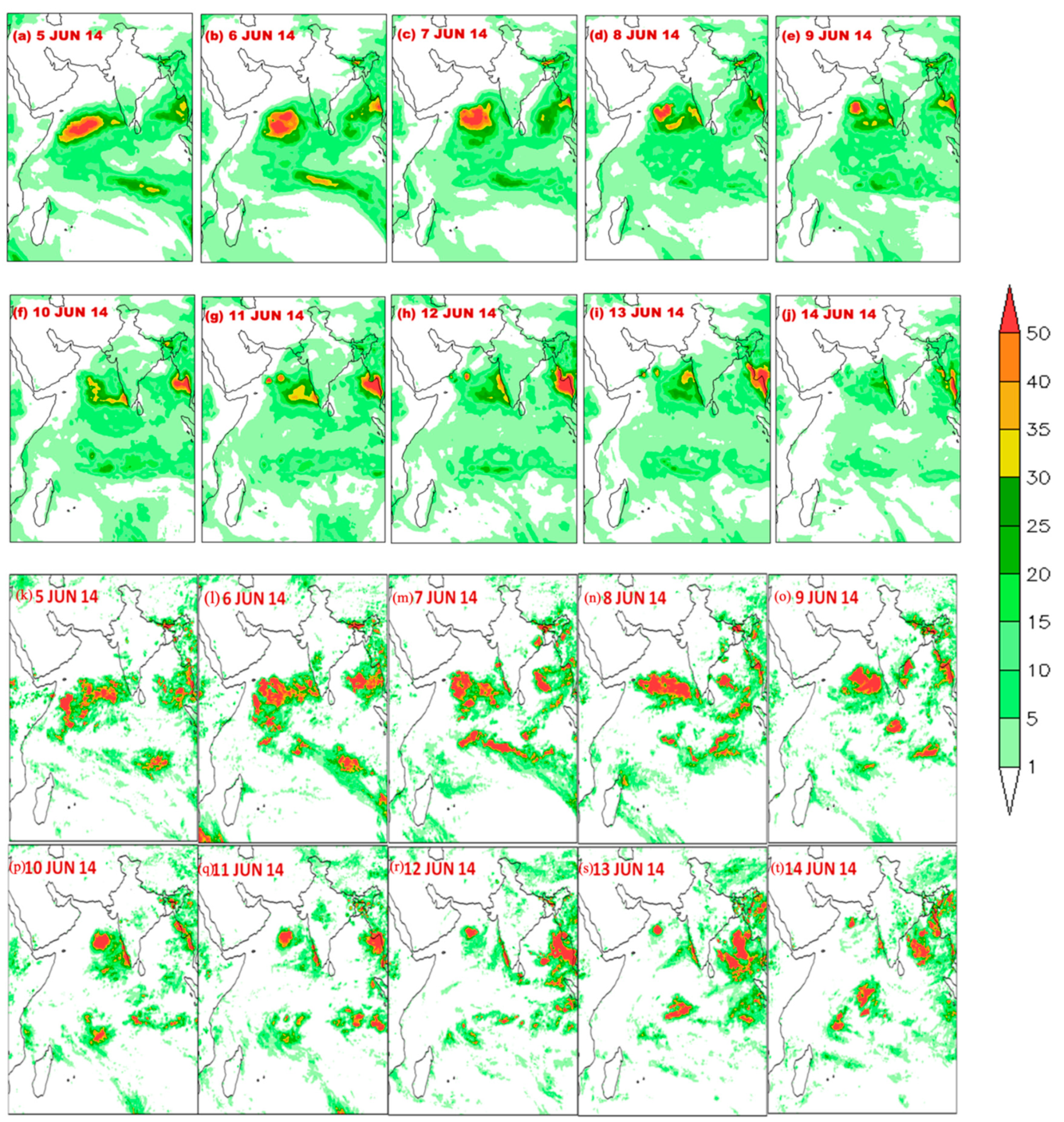
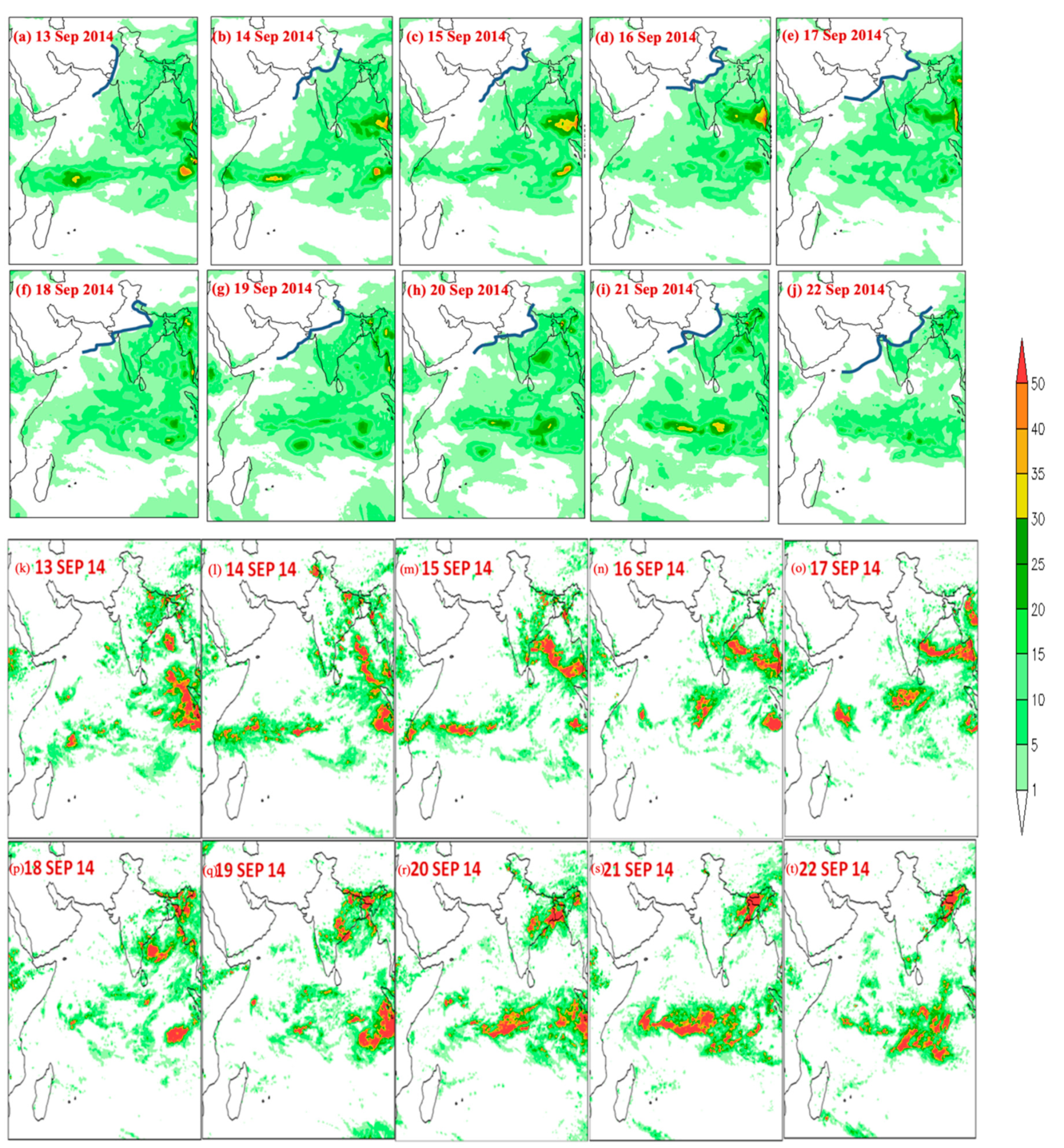
The above figure points out the incapability of numerical weather prediction models to accurately represent the observed rainfall. They either overestimate or underestimate the rainfall values. The location of precipitation maxima does not agree with observation closely. Only SE and ECMWF were able to capture the event adequately in terms of area. Skill forecasts of precipitation demonstrate that it is possible to obtain higher skills for precipitation forecasts for days 1 through 10 of projections from the use of the SE compared to the best model in the suite. The higher skills of the SE make it a handy tool for such real-time events. The following two examples, each shown as a spatial distribution of the SE on the onset date (5 June 2014) and on the demise date (13 September 2014). These are seen in the form of spatiotemporal position on Figure 4a–j and Figure 5a–j with the corresponding TRMM observed shown on Figure 4k–t and Figure 5k–t of the Indian summer monsoon during the forecast span of 10 days from day 1 to day 10, respectively.
The above work is materialized in real-time, and one example of ten SE precipitation forecast valid at 12 UTC (05–14 June) onset date is shown in Figure 4. After the onset date (5 June 2014), the monsoon’s progress can be seen over the Indian landmass. Another example in Figure 5 for monsoon Isochrones’ withdrawal (blue lines) for 13 September 2014 is shown from SE forecasts. The SE forecast shows a systematic withdrawal of the southwest monsoon.
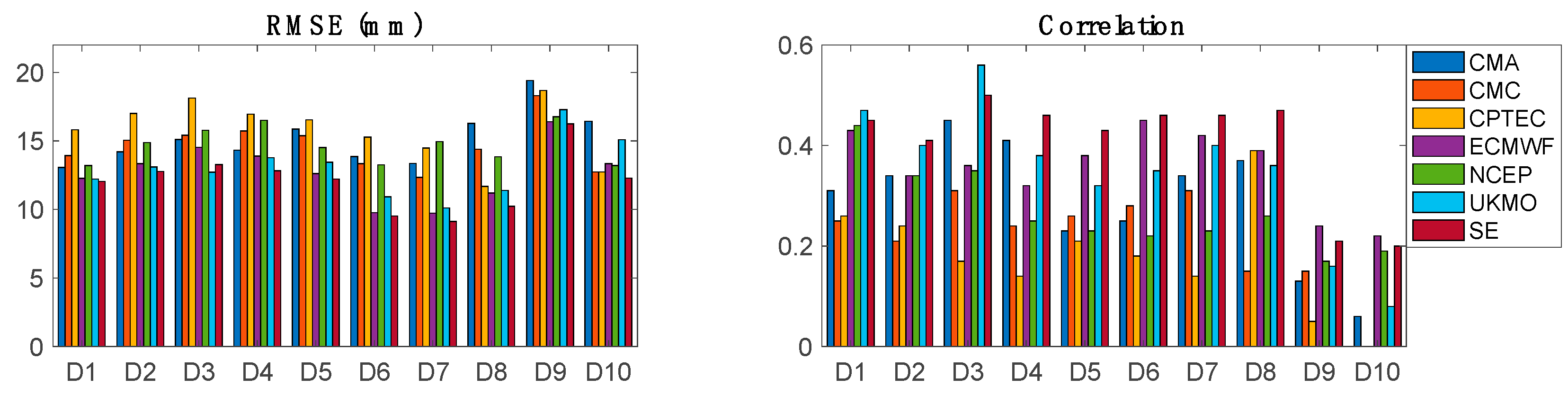
Prediction of the onset day of the Indian summer monsoon rainfall remains an important topic for monsoon meteorologists. Figure 6 shows the RMSE and correlation on 5 June 2014 up to day 10. SE carries the lowest RMSE and highest correlation from day 1 to day 10. Among six member models, SE carries the lowest RMSE of 8.5 mm/day and highest correlation of 0.49.
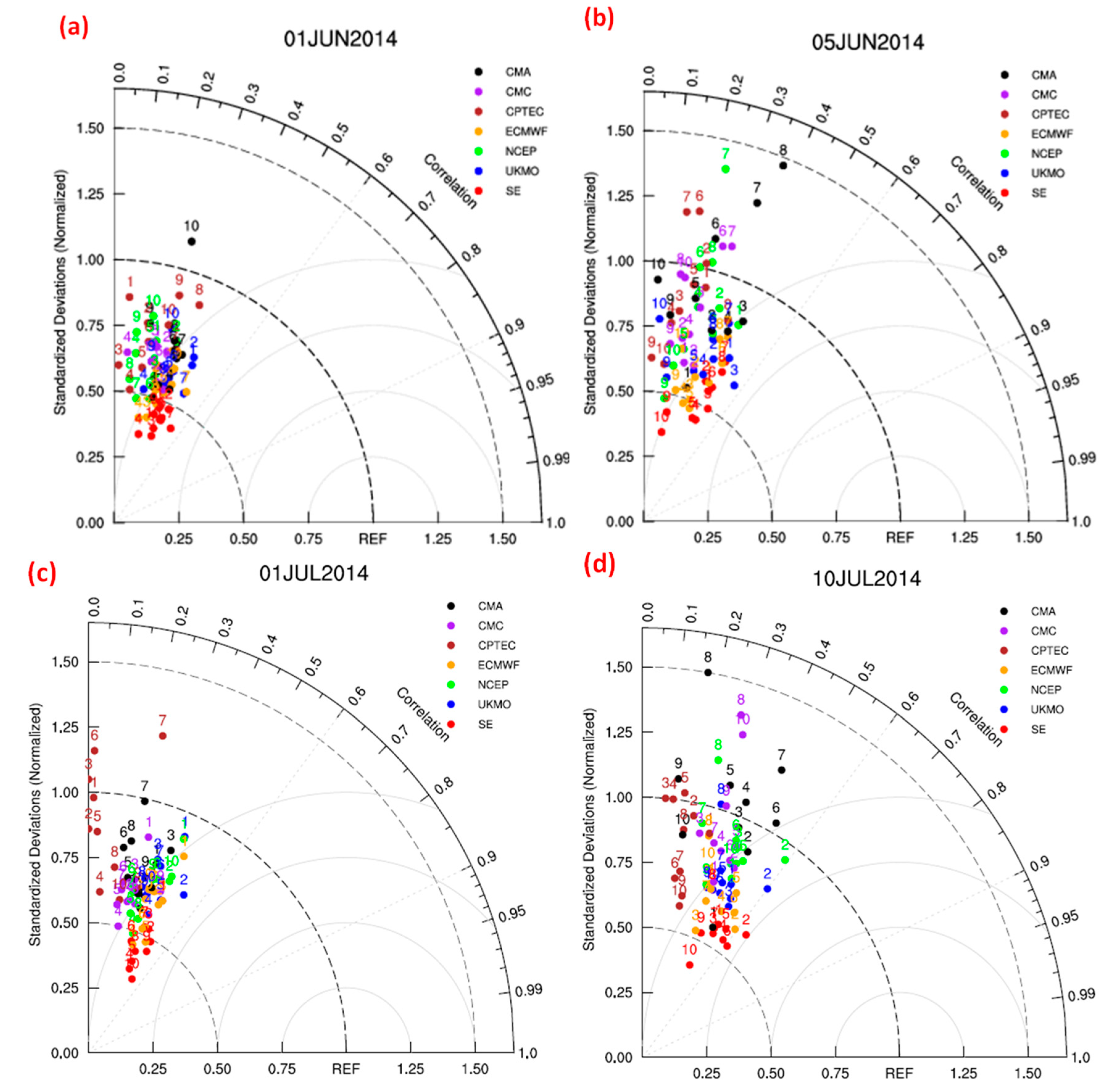
We have shown the qualitative effect of the spatial distribution of rainfall, which we further quantitatively demonstrated in the form of their systematic errors, root mean square errors, and their standard deviations from the observed. All these quantitative numbers can be combined in the form of a Taylor diagram. Figure 7a–d show skills based on the Taylor diagram [25] for the few case studies of dates 01 June 2014, 05 June 2014, 01 July 2014, and 10 July 2014. This is a polar diagram. The radial direction carries a normalized standard deviation of the forecasts of all models and SE (normalized concerning the observed TRMM rainfall estimates for each day). The azimuth in these four diagrams carries the spatial correlation of the forecasts. These are forecasts from day 1 to day 10 assigned to each day’s forecast with a single dot with the forecast day number. The color scheme is explained in the legend of the illustration. Values closer to 0 for the normalized deviation denote a good forecast, and values closer to the REF point along the azimuth are good forecasts [25].
Figure 7 shows the normalized values of the RMSE, correlation, and standard deviation from day 1 to day 8 of the forecast on four selected days of 2014. The clustering of importance relative to these optimal skills is best seen for the SE denoted by red dots. The member models show a more extensive spread of errors in comparison. A careful glance at the case study starting on 01 June 2014 in Figure 7a show the clustering of red points for ten days. This refers to the degradation of skill scores, being the least in the case of SE, whereas all other models show a large spread of metric points, which indicates a relatively fast decreasing skills with time for member models. Similar information can be drawn from the other cases in Figure 7b–d. It is also observed from the results that ECMWF forecasts outperform all other ensemble members, and the CPTEC model forecast shows the lowest skill in terms of Root Mean Square Error (RMSE) and Correlation Coefficient (CC). The overall conclusion drawn from the Taylor diagram is that SE techniques possess the best skill score for domain-averaged rainfall. SE shows a standard deviation of ~0.42mm and correlation of ~0.49 for 05 June 2014, on the onset day of the Indian monsoon. We have developed a real-time package that can be used for the forecast of rainfall two weeks in advance, consisting of six ensemble members with the option to add more members. We have also submitted SE forecasts to the USA-based company Weather Predict Consulting Inc. for the complete season (JJAS) of 2014.
4. Conclusions
SE as a postprocessing tool reduces the systematic biases from a suite of member models to provide a better forecast. This study consists of six global models’ datasets bilinearly interpolated to 25km of horizontal resolution. The comparison and analysis are made among member models and SE. Among member models, ECMWF and UKMO perform equally well with rainfall prediction. It is possible to acquire day 1 to day 10 rainfall prediction with greater confidence than a single model using the SE technique. The skill of the performance of the prediction degrades from day 1 to day 10. It does not decrease monotonously.
The limitation of SE is that its skill depends on the skills of constituting member models. Therefore, high-skill member models are required to improve the SE forecasts further. On the onset day (05 June 2014) of the Indian summer monsoon, SE shows a standard deviation of ~0.42mm, correlation of 0.49, and RMSE 8.5 mm, which is the best among all member models. Ensemble techniques could be regarded as an objective way to extract information from the history of constituting models and improving future predictions. In addition to the aforementioned SE technique, there are many other methods available for preparing suited statistics from the record for future forecast improvement [26,27,28]. However, statistical methods have certain limitations though, e.g., the SE forecast is not suitable for extreme events if models cannot predict them; therefore, it becomes vital to improve the single model forecast itself. To use the Observing Systems Capability Analysis and Review (OSCAR) tool for geophysical variables, which have the qualities of uncertainty, horizontal resolution, vertical resolution, observing period, timeliness, and stability, the system must first have perfect acquisition of the data. SE depends on the models used in the mixture models. Besides the enhancement in horizontal and vertical resolution of the datasets, the consistency of the final forecast product also improved. Finally, the forecast data from SE are extremely promising for any kind of time-scale data such as from minutes to the decadal scale.
Author Contributions
A.B. provided the idea, wrote the manuscript, and created the figures. V.K. wrote the manuscript and made the figures, A.S. did the work of editing and writing, T.S. did the work of editing and supervision, S.P.S. did the work of editing and analysis. All authors have read and agreed to the published version of the manuscript.
Funding
At present, we do not have any budget for this research work.
Acknowledgments
The author gratefully acknowledges the provision of the computing facility to carry out this work at the Centre for Atmospheric Sciences at IIT Delhi and Florida State University (FSU), Tallahassee.
Conflicts of Interest
The authors declare no conflict of interest.
References
- Jayakumar, A.; Kumar, V.; Krishnamurti, T.N. Lead time for medium range prediction of the dry spell of monsoon using multi-models. J. Earth Syst. Sci. 2013, 122, 991–1004. [Google Scholar] [CrossRef] [Green Version]
- Kipkogei, O.; Bhardwaj, A.; Kumar, V.; Ogallo, L.A.; Opijah, F.J.; Mutemi, J.N.; Krishnamurti, T.N. Improving multimodel medium range forecasts over the Greater Horn of Africa using the FSU superensemble. Meteorol. Atmos. Phys. 2016, 128, 441–451. [Google Scholar] [CrossRef]
- Krishnamurti, T.N. Weather and Seasonal Climate Prediction of Asian Summer Monsoon. Review Topic B1a: Numerical Modeling-Forecast. 2005, pp. 1–34. Available online: http://danida.vnu.edu.vn/cpis/files/Refs/Seasonal_FCS/WEATHER%20AND%20SEASONAL%20CLIMATE%20PREDICTION%20OF%20ASIAN%20SUMMER%20MONSOON.pdf (accessed on 10 January 2021).
- Sikka, D.R. Two Decades of Medium-Range Weather Forecasting in India: National Centre for Medium-Range Weather Forecasting; COLA Technical Report 276; Center of Ocean-Land-Atmosphere Studies: Fairfax, VA, USA, 2009; p. 100. [Google Scholar]
- Palmer, T.N.; Shutts, G.J.; Hagedorn, R.; Doblas-Reyes, F.J.; Jung, T.; Leutbecher, M. Representing model uncertainty in weather and climate prediction. Annu. Rev. Earth Planet. Sci. 2005, 33, 163–193. [Google Scholar] [CrossRef]
- Warner, T.T. Numerical Weather and Climate Prediction; Cambridge University Press: Cambridge, UK, 2010; p. 259. [Google Scholar]
- Kalnay, E.; Kanamitsu, M.; Baker, W.E. Global numerical weather prediction at the National Meteorological Center. Bull. Am. Meteorol. Soc. 1990, 71, 1410–1428. [Google Scholar] [CrossRef]
- Krishnamurti, T.N.; Biswas, M.K.; Mackey, B.P.; Ellingson, R.G.; Ruscher, P. Hurricane forecasts using a suite of large-scale models. Tellus A 2011, 63, 727–745. [Google Scholar] [CrossRef]
- Krishnamurti, T.N.; Kumar, V.; Simon, A.; Bhardwaj, A.; Ghosh, T.; Ross, R. A review of multimodel superensemble forecasting for weather, seasonal climate, and hurricanes. Rev. Geophys. 2016, 54, 336–377. [Google Scholar] [CrossRef]
- Acharya, N.; Kar, S.C.; Kulkarni, M.A.; Mohanty, U.C.; Sahoo, L.N. Multi-model ensemble schemes for predicting northeast monsoon rainfall over peninsular India. J. Earth Syst. Sci. 2011, 120, 795–805. [Google Scholar] [CrossRef]
- Kumar, A.; Mitra, A.K.; Bohra, A.K.; Iyengara, G.R.; Duraib, V.R. Multi-model ensemble (MME) prediction of rainfall using neural networks during monsoon season in India. Meteorol. Appl. 2012, 19, 161–169. [Google Scholar] [CrossRef]
- Kirtman, B.P.; Min, D.; Infanti, J.M.; Kinter, J.L.; Paolino, D.A.; Zhang, Q.; van den Dool, H.; Saha, S.; Mendez, M.P.; Becker, E.; et al. The North American multi-model ensemble. Bull. Amer. Met. Soc. 2014, 15, 529–550. [Google Scholar]
- Min, Y.-M.; Kryjov, V.N.; Oh, S.M. Assessment of APCC multimodel ensemble prediction in seasonal climate forecasting: Retrospective (1983– 2003) and real-time forecasts (2008 –2013). J. Geophys. Res. Atmos. 2014, 119, 12123–12150. [Google Scholar] [CrossRef]
- Bougeault, P.; Toth, Z.; Bishop, C.; Brown, B.; Burridge, D.; Chen, D.H.; Ebert, B.; Fuentes, M.; Hamill, T.M.; Mylne, K.; et al. The THORPEX interactive grand global ensemble. Bull. Am. Meteorol. Soc. 2010, 91, 1059–1072. [Google Scholar] [CrossRef]
- McBride, J.L.; Ebert, E.E. Verification of quantitative precipitation forecasts from operational numerical weather prediction models over Australia. Weather Forecast. 2000, 15, 103–121. [Google Scholar] [CrossRef]
- Doswell, C.A., III; Davies-Jones, R.; Keller, D.L. On summary measures of skill in rare event forecasting based on contingency tables. Weather Forecast. 1990, 5, 576–585. [Google Scholar] [CrossRef] [Green Version]
- Hou, A.Y.; Skofronick-Jackson, G.; Kummerow, C.D.; Shepherd, J.M. Global precipitation measurement. In Precipitation: Advances in Measurement, Estimation and Prediction; Springer: Berlin/Heidelberg, Germany, 2008; pp. 131–169. [Google Scholar]
- Huffman, G.J.; Adler, R.F.; Bolvin, D.T.; Nelkin, E.J. The TRMM multi-satellite precipitation analysis (TMPA). In Satellite Rainfall Applications for Surface Hydrology; Springer: Dordrecht, The Netherlands, 2010; pp. 3–22. [Google Scholar]
- Richardson, D.; Buizza, R.; Hagedorn, R. First Workshop on the THORPEX Interactive Grand Global Ensemble (TIGGE); World Meteorological Organization: Geneva, Switzerland, 2005; Volume 1, p. 39. [Google Scholar]
- Huffman, G.J.; Bolvin, D.T.; Nelkin, E.J.; Wolff, D.B.; Adler, R.F.; Gu, G.; Hong, Y.; Bowman, K.P.; Stocker, E.F. The TRMM multisatellite precipitation analysis (TMPA): Quasi-global, multiyear, combined-sensor precipitation estimates at fine scales. J. Hydrometeorol. 2007, 8, 38–55. [Google Scholar] [CrossRef]
- Matsueda, M.; Hirokazu, E. Verification of medium-range MJO forecasts with TIGGE. Geophys. Res. Lett. 2011, 38, 1548–1550. [Google Scholar] [CrossRef] [Green Version]
- Yun, W.T.; Stefanova, L.; Krishnamurti, T.N. Improved weather and seasonal climate forecasts from a multimodel superensemble. Science 1999, 285, 1548–1550. [Google Scholar]
- Yun, W.T.; Stefanova, L.; Krishnamurti, T.N. Improvement of the superensemble technique for seasonal forecasts. J. Clim. 2003, 16, 3834–3840. [Google Scholar] [CrossRef]
- Krishnamurti, T.N.; Mishra, A.K.; Chakraborty, A.; Rajeevan, M. Improving Global Model Precipitation Forecasts over India Using Downscaling and the FSU Superensemble. Part I: 1–5-Day Forecasts. Mon. Weather Rev. 2009, 137, 2713–2735. [Google Scholar] [CrossRef] [Green Version]
- Taylor, K.E. Summarizing multiple aspects of model performance in a single diagram. J. Geophys. Res. Atmos. 2001, 106, 7183–7192. [Google Scholar] [CrossRef]
- Roy Bhowmik, S.K.; Durai, V.R. Multi-model ensemble forecasting of rainfall over Indian monsoon region. Atmosfera 2008, 21, 225–239. [Google Scholar]
- Acharya, N.; Chattopadhyay, S.; Mohanty, U.C.; Dash, S.K.; Sahoo, L.N. On the bias correction of general circulation model output for Indian summer monsoon. Meteorol. Appl. 2013, 20, 349–356. [Google Scholar] [CrossRef]
- Acharya, N.; Shrivastava, N.A.; Panigrahi, B.K.; Mohanty, U.C. Development of an artificial neural network based multi-model ensemble to estimate the northeast monsoon rainfall over south peninsular India: An application of extreme learning machine. Clim. Dyn. 2014, 43, 1303–1310. [Google Scholar] [CrossRef]
Figure 1.
This figure shows the % of discrepancies from different models with 95% CI for precipitation predictions valid from day 1 to day 10.
Figure 1.
This figure shows the % of discrepancies from different models with 95% CI for precipitation predictions valid from day 1 to day 10.

Figure 2.
represent (a) the stability analysis of spatial average coefficients and (b–g) spatial distribution of coefficients after training of 600 days, consisting of six member models in the training phase of the multimodel SE.
Figure 2.
represent (a) the stability analysis of spatial average coefficients and (b–g) spatial distribution of coefficients after training of 600 days, consisting of six member models in the training phase of the multimodel SE.

Figure 3.
Spatial plot of observed TRMM, SE, and member models precipitation (mm) for 5 June 2014 (day one), 12 UTC.
Figure 3.
Spatial plot of observed TRMM, SE, and member models precipitation (mm) for 5 June 2014 (day one), 12 UTC.

Figure 4.
First two rows (a–j) are ten days’ real-time SE forecast, and the last two rows (k–t) from TRMM observed precipitation (mm) 12UTC (05–14 June).
Figure 4.
First two rows (a–j) are ten days’ real-time SE forecast, and the last two rows (k–t) from TRMM observed precipitation (mm) 12UTC (05–14 June).

Figure 5.
First two rows (a–j) are ten days’ real-time SE forecast, and the last two rows (k–t) from TRMM observed precipitation (mm) 12UTC (13–22 Sep).
Figure 5.
First two rows (a–j) are ten days’ real-time SE forecast, and the last two rows (k–t) from TRMM observed precipitation (mm) 12UTC (13–22 Sep).

Figure 6.
Performance of member model and SE on onset day of Indian summer monsoon of 05 June 2014 (a) RMSE, (b) correlation.
Figure 6.
Performance of member model and SE on onset day of Indian summer monsoon of 05 June 2014 (a) RMSE, (b) correlation.

Figure 7.
Four examples of ten-day forecasts of member models (colored dot) and the SE (red dots) are shown in the Taylor diagram. The radial axis denotes the normalized standard deviations and the azimuthal coordinate represents the spatial correlations. This illustration includes results for (a) 1 Jun. 2014, (b) 5 Jun. 2014, (c) 1 Jul. 2014, and (d) 10 Jul. 2014; the dates of the forecast are identified by small print forecast days.


Table 1.
Lists of the main characteristics of the six selected ensemble prediction systems in this study.
Table 1.
Lists of the main characteristics of the six selected ensemble prediction systems in this study.
| Centers | Horizontal Resolution | Vertical Resolution | Ensemble Members | Initial Condition Perturbations | Forecast Length | Forecast Frequency | Start Date |
|---|---|---|---|---|---|---|---|
| CMA (China) | T213 (0.5625) | 31 | 14 | BVs (globe) | 10 days | 12 UTC | 15 May 2007 |
| CMC (Canada) | TL149 (1.2°) | 28 | 20 | EnKF (globe) | 16 days | 12 UTC | 03 Oct. 2007 |
| CPTEC (Brazil) | T126 (0.9474°) | 28 | 14 | EOF (45S-30N) | 15 days | 12 UTC | 01 Feb. 2008 |
| ECMWF (Europe) | TL399 (0.45°) TL255 (0.7°) | 62 | 50 | SVs (globe) | 0–10 days 10–15 days | 12 UTC | 01 Oct. 2006 |
| NCEP (USA) | T126 (0.9474°) | 28 | 20 | ET (globe) | 16 days | 12 UTC | 05 Mar. 2007 |
| UKMO (UK) | 1.25° × 0.83° | 38 | 23 | ETKF (globe) | 15 days | 12 UTC | 01 Oct. 2006 |
Publisher’s Note: MDPI stays neutral with regard to jurisdictional claims in published maps and institutional affiliations. |
© 2021 by the authors. Licensee MDPI, Basel, Switzerland. This article is an open access article distributed under the terms and conditions of the Creative Commons Attribution (CC BY) license (http://creativecommons.org/licenses/by/4.0/).
Share and Cite
MDPI and ACS Style
Bhardwaj, A.; Kumar, V.; Sharma, A.; Sinha, T.; Singh, S.P. Application of Multimodel Superensemble Technique on the TIGGE Suite of Operational Models. Geomatics 2021, 1, 81-91. https://0-doi-org.brum.beds.ac.uk/10.3390/geomatics1010007
AMA Style
Bhardwaj A, Kumar V, Sharma A, Sinha T, Singh SP. Application of Multimodel Superensemble Technique on the TIGGE Suite of Operational Models. Geomatics. 2021; 1(1):81-91. https://0-doi-org.brum.beds.ac.uk/10.3390/geomatics1010007
Chicago/Turabian StyleBhardwaj, Amit, Vinay Kumar, Anjali Sharma, Tushar Sinha, and Surendra Pratap Singh. 2021. "Application of Multimodel Superensemble Technique on the TIGGE Suite of Operational Models" Geomatics 1, no. 1: 81-91. https://0-doi-org.brum.beds.ac.uk/10.3390/geomatics1010007