Transfer Learning for LiDAR-Based Lane Marking Detection and Intensity Profile Generation

Abstract

Recently, light detection and ranging (LiDAR)-based mobile mapping systems (MMS) have been utilized for extracting lane markings using deep learning frameworks. However, huge datasets are required for training neural networks. Furthermore, with accurate lane markings being detected utilizing LiDAR data, an algorithm for automatically reporting their intensity information is beneficial for identifying worn-out or missing lane markings. In this paper, a transfer learning approach based on fine-tuning of a pretrained U-net model for lane marking extraction and a strategy for generating intensity profiles using the extracted results are presented. Starting from a pretrained model, a new model can be trained better and faster to make predictions on a target domain dataset with only a few training examples. An original U-net model trained on two-lane highways (source domain dataset) was fine-tuned to make accurate predictions on datasets with one-lane highway patterns (target domain dataset). Specifically, encoder- and decoder-trained U-net models are presented wherein, during retraining of the former, only weights in the encoder path of U-net were allowed to change with decoder weights frozen and vice versa for the latter. On the test data (target domain), the encoder-trained model (F1-score: 86.9%) outperformed the decoder-trained (F1-score: 82.1%). Additionally, on an independent dataset, the encoder-trained one (F1-score: 90.1%) performed better than the decoder-trained one (F1-score: 83.2%). Lastly, on the basis of lane marking results obtained from the encoder-trained U-net, intensity profiles were generated. Such profiles can be used to identify lane marking gaps and investigate their cause through RGB imagery visualization.

1. Introduction

The development of autonomous vehicles (AVs) and advanced driver assistance systems (ADASs) has prompted the development of high-definition (HD) maps with attributes such as crosswalks, signalized intersections, and bike lanes [1]. Lane markings are essential elements of these maps and, thus, their extraction is necessary. Lane markings are also vital for road management, providing well-defined lanes for navigating roads safely in day and night conditions [2]. Traffic accidents have increased in densely populated urban areas with worn-out lane markings [3]. To mitigate these accidents, it is imperative to provide the current condition of lane markings along the road surface. While several studies have been conducted to detect lane markings through images and videos, light detection and ranging (LiDAR) point clouds have attracted significant attention from the research community due to the availability of reflective properties of lane markings in LiDAR data unlike images, which could be affected by weather and lighting conditions. Additionally, highly accurate, dense point-cloud data can be obtained in a short time interval without being affected by occlusions, lighting, and weather. Moreover, on the basis of the geometric and reflectivity information provided by LiDAR scanners, the intensity information of extracted lane markings can be automatically reported. Such information is valuable for transportation agencies since it will reduce the number of on-site inspections whereby lane marking gaps can be identified, and their causes can be investigated through coacquired imagery visualization, thereby saving manual labor and ensuring personnel safety. Hence, a strategy for generating intensity profiles, as well as investigating the cause of lane marking gaps, is required.

LiDAR-based lane marking extraction approaches are based on either derived 2D intensity images [4,5] or original 3D point clouds as input [6,7,8]. Traditionally, these strategies focus on finding an optimum intensity threshold that separates lane marking points from non-lane marking ones. However, LiDAR point-cloud intensity depends on multiple factors such as the sensor-to-object range, laser beam incidence angle, and reflective properties of the scanned surface. Thus, intensity values must be corrected/normalized for determining an effective threshold [9]. Höfle et al. [10] proposed two approaches for intensity data correction: (a) data-based correction where homogeneous surfaces were used to empirically estimate parameters for a correction function accounting for range-dependent factors, and (b) model-based correction where intensity values were corrected according to the physical principle of radar systems. Another range-dependent intensity correction was proposed by Tan et al. [11]. They substituted the theoretical model (intensity dependence on the inverse of squared ranges) with a polynomial function in the range. The degree of the polynomial, together with its coefficients, was determined for each sensor by least-squares adjustment. Krooks et al. [12] studied the effect of incidence angle on LiDAR intensity and found that such an effect is independent of the sensor-to-object distance and, thus, can be corrected separately. Bolkas et al. [13] modeled diffused and specular reflection from different colored surfaces through a Torrance–Sparrow model [14]. They used the specular reflection component and incidence angle to correct the intensity data. However, even after intensity correction through various strategies proposed in the literature, one must have prior information about intensity distribution for LiDAR-based lane marking extraction approaches to be effective. Recently, the focus has shifted to applying deep learning in the form of novel convolutional neural network (CNN) architectures for lane marking extraction that are agnostic to LiDAR intensity correction or prior knowledge about intensity distribution. However, a huge dataset is required to train CNNs, which is often a major bottleneck as manual effort is required for labeling input data [15,16]. Cheng et al. [17], thus, proposed a strategy to automatically label intensity images for lane marking extraction. They first normalized LiDAR point-cloud intensity using the procedure proposed by Levinson [18]. Thereafter, a fixed intensity threshold was applied, followed by noise removal to extract lane markings. The lane marking point clouds were then rasterized into intensity images to serve as labels for training a U-net model.

In addition to requiring a large number of training samples, another drawback of CNNs is their inability to generalize to patterns that are significantly different from ones encountered during training even after application of techniques such as dropout (a technique where neurons in a neural network are randomly dropped during training to prevent overfitting), weight regularization (set of techniques that prevent the neural network weights from growing too large so that network is not highly sensitive to small changes in input), and data augmentation (set of techniques where training data size is increased by adding modified copies of existing training samples) [19,20,21]. Thus, transfer learning has gained more interest where the current knowledge can be adapted to new conditions for better prediction [22,23]. In the geospatial domain, many researchers have utilized a pretrained network to solve their problems of interest. Yuan et al. [24] first trained a CNN to learn the nonlinear mapping from low-resolution RGB images to high-resolution ones. The same network was then transferred to hyperspectral images by tackling bands individually. Chen et al. [25] used a Visual Geometry Group-16 model (VGG16) pretrained on the ImageNet dataset (a database of 14 million annotated images over 20,000 miscellaneous categories) for airplane detection in remote sensing images. They replaced the fully connected layers of the model with additional convolutional layers and retrained the model on a small number of manually labeled airplane samples. Nezafat et al. [26] investigated three networks (AlexNet, VGGNet, and ResNet) pretrained on the ImageNet dataset to classify truck images, generated from LiDAR point-cloud data, according to their body type. Low-level features extracted as output from each pretrained model were fed as input to train a multilayer perceptron (MLP) for truck body type classification.

It is, thus, evident that a model trained on a dataset can be adapted to perform predictions on a new dataset through changes in architecture and retraining with few examples. This is significant in the context of deep learning-based lane marking extraction in LiDAR intensity images. Since the intensity of LiDAR data and lane marking patterns vary from one dataset to another, it is not practical and efficient to train a model from scratch for every newly collected dataset, even with an automated labeling procedure. Thus, the objectives of this paper are (1) to study fine-tuning of a pretrained U-net model for knowledge transfer from the source to target domain in the context of lane marking extraction, and (2) to propose an intensity profile generation strategy utilizing the lane marking predictions by the fine-tuned U-net model.

In detail, a transfer learning strategy is applied for lane marking extraction whereby a pretrained U-net model from a previous study [17] is fine-tuned with additional training samples from another dataset consisting of new lane marking patterns (not seen earlier during the training phase of the pretrained model). This is an example of domain adaptation where the task in the two settings remains the same (here, the task being lane marking extraction) but input distribution is different. The pretrained U-net model was trained on the past dataset collected over two-lane highways (hereafter referred to as “source domain dataset”). The new dataset (hereafter also referred to as “target domain dataset”) includes other lane marking patterns such as one-lane highways and dual lane markings at the edge of the road surface, in addition to two-lane highways. Specifically, the main contributions of this study are as follows:

• A transfer learning approach is successfully applied to fine-tune weights of a pre-trained U-net model with limited training data for lane marking extraction on a target domain dataset under two scenarios:
  • only encoder is trained with decoder weights frozen;
  • only decoder is trained with encoder weights frozen.
• The predictions of both transfer learning models are compared with each other. In addition, the fine-tuned models are also evaluated upon the source domain dataset with two-lane highways, and their performance is compared with the pretrained model. This helped in assessing the generalization ability of the two models. Moreover, these performance comparisons aided in assessing the preferable modes of fine-tuning U-net for domain adaptation. To the best of authors’ knowledge, most transfer learning strategies deal with networks that are not fully convolutional unlike U-net. Moreover, U-net fine-tuning has only been studied in the biomedical context [27].
• To clearly illustrate the benefits of fine-tuning, another U-net model is trained from scratch on source and target domain datasets, and then its predictions are compared with the fine-tuned models on target domain datasets.
• Lastly, intensity profiles are generated along the road datasets utilized in this study. Regions with lane marking gaps are reported along with the corresponding RGB image visualization. This procedure assists in lane marking inspection, and it removes the possibility of missed problematic areas during manual inspection.

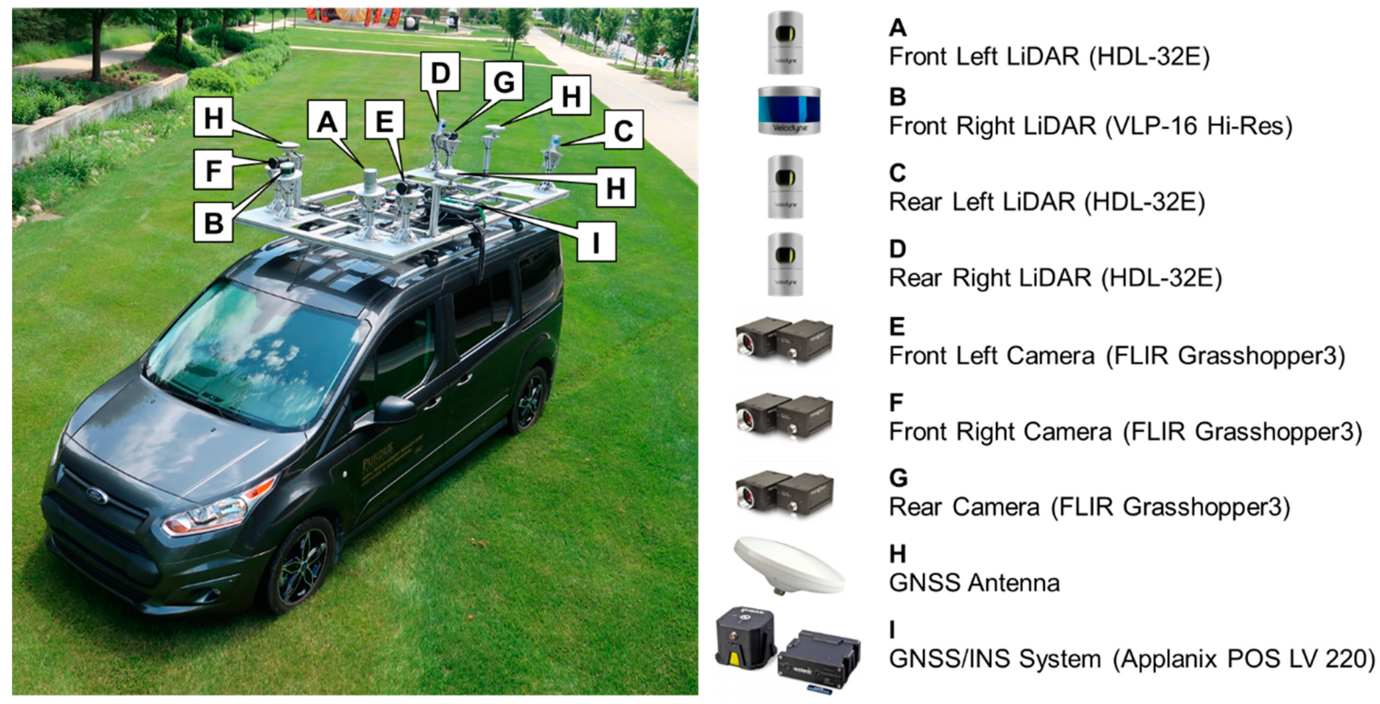
The rest of this paper is structured as follows: first, the mobile mapping system and collected LiDAR point clouds used in this study are described in Section 2. The motivation for U-net fine-tuning is presented in Section 3, followed by Section 4 that introduces the proposed strategies. Lastly, the results are reported and discussed in Section 5, while the conclusions and scope for future work are summarized in Section 6.

2. Mobile LiDAR System and Datasets Used in This Research

2.1. Mobile LiDAR System

In this study, a mobile mapping system—Purdue Wheel-Based Mobile Mapping System, High Accuracy (PWMMS-HA)—is utilized. The PWMMS-HA (shown in Figure 1) has four 3D LiDAR units onboard: three Velodyne HDL-32Es and one Velodyne VLP-16 High Resolution. The system is also equipped with three FLIR Grasshopper3 9.1MP GigE color cameras. The remote sensing units of the PWMMS-HA are directly georeferenced by an Applanix POS LV 220 global navigation satellite system/inertial navigation system (GNSS/INS) unit (i.e., the position and orientation information of the remote sensing units throughout the survey mission are directly derived by the GNSS/INS mounted on the PWMMS-HA). The post-processing positional accuracy of the POS LV 220 is ±2 cm, and the attitude accuracy is 0.02° and 0.025° for the roll/pitch and heading, respectively [28]. The range accuracy measures for the HDL-32E and VLP-16 are ±2 cm and ±3 cm, respectively [29,30]. The onboard cameras are triggered through the pulse per second (PPS) output of the POS LV which is fed as an input to the Grasshopper3’s optoisolated general-purpose input/output (GPIO). Event feedback for both systems is provided directly from the cameras to the GNSS/INS systems through the strobe feedback GPIO. PointGrey FlyCap is used as the software interface for all cameras during data collection.

Through a system calibration procedure, mounting parameters between LiDAR units and an Applanix POSLV 220 GNSS/Inertial Measurement Unit (IMU) navigation system were estimated, facilitating the reconstruction of georeferenced, well-registered point clouds from the LiDAR scanners [31]. The cameras’ mounting parameters were estimated through another calibration procedure for LiDAR point-cloud registration with imagery [32]. Those parameters combined with vehicle trajectory enable forward and backward projection between the reconstructed point cloud and RGB imagery. The projection capability aids in analyzing the lane marking extraction performance of various U-net models and lane marking gaps identified through intensity profiling. In Figure 2, the correspondence between a road surface point cloud and RGB imagery is shown, where the red dot in the former is projected onto the latter (displayed as an empty magenta circle). Hereafter, a red dot represents a location in the LiDAR point cloud, while a magenta circle corresponds to the same location in an RGB image.

2.2. Dataset Description

For fine-tuning, the pretrained U-net model from a prior study [17] was adopted. This model was trained on three datasets where the first two belonged to an interstate highway and the third covered a rural highway. They are referred to as datasets 1, 2, and 3, which covered 18.04, 33.87, and 15.29 miles, respectively. The locations of these datasets are shown in Figure 3. In the past study, samples from datasets 1 and 3 were utilized for training, and samples from dataset 2 were used for testing. All these datasets were collected over two-lane highways, as illustrated by the RGB images in Figure 4.

The target domain datasets used in this study were collected on highway and non-highway roads in Tippecanoe County in Indiana, USA. The northbound (NB) and southbound (SB) segments, displayed as red and blue trajectories in Figure 5, were collected along a highway with a total length of 16.1 and 11.8 miles, respectively. The eastbound (EB) and westbound (WB) segments, denoted as yellow and magenta trajectories in Figure 5, belonged to non-highway areas with a total length of 5 miles each. In addition to two-lane highways, this dataset also included lane marking patterns such as (a) one-lane highway with dual lane marking at the center, (b) dual lane markings at the road edge, and (c) pair of dual lane markings at the road edge. These patterns were not seen in the source domain dataset, which was used for the training of the U-net model. RGB images of the new lane marking patterns are shown in Figure 6. Lastly, a completely unseen dataset (hereafter referred to as “independent dataset”) not belonging to either source or target domain dataset locations was utilized to further evaluate the generalization capability of U-net models and demonstrate the benefit of fine-tuning a pretrained model. This dataset was acquired over a rural highway, including both one- and two-lane areas, as shown in Figure 7.

3. Motivation for U-Net Fine-Tuning

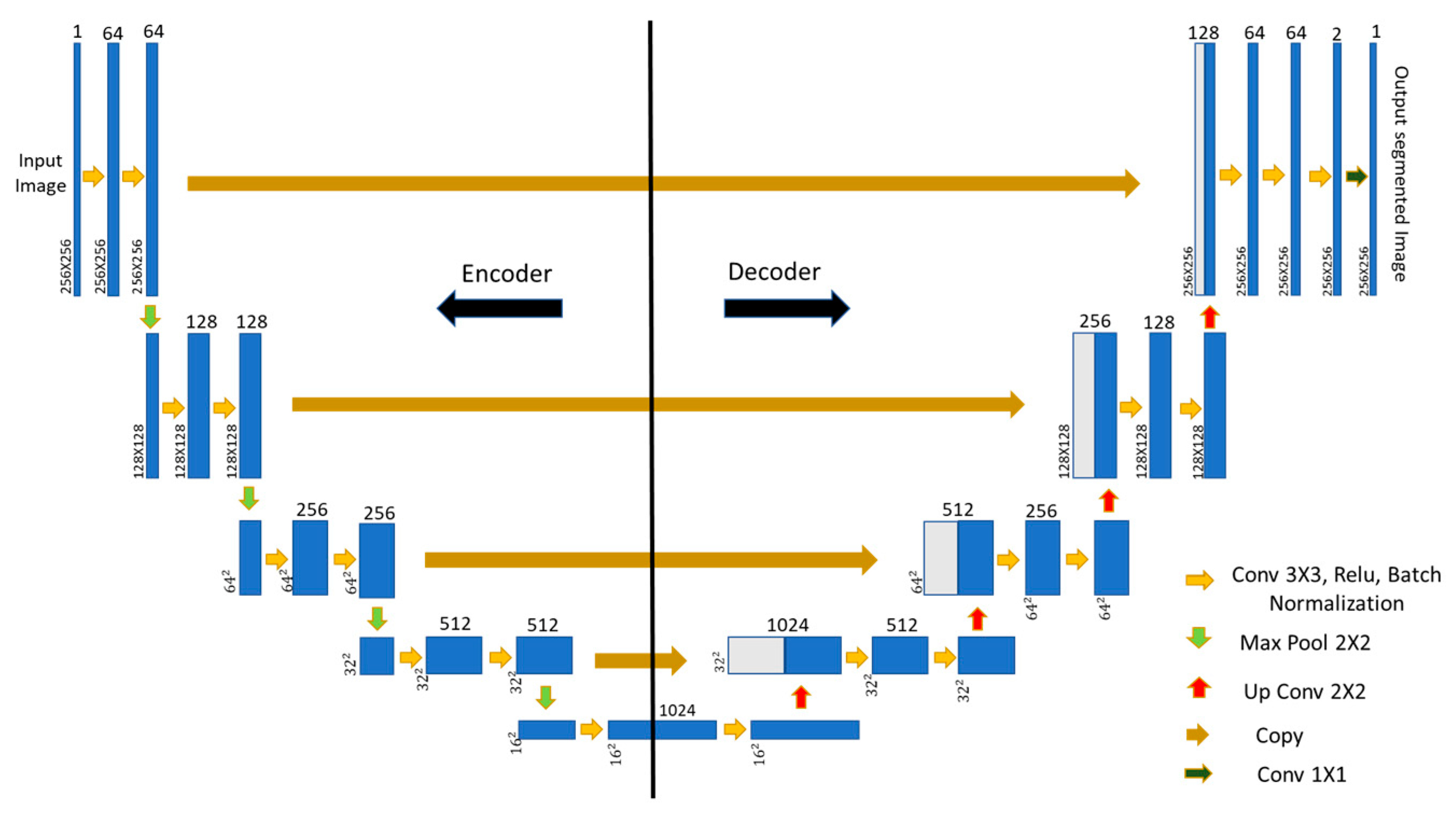
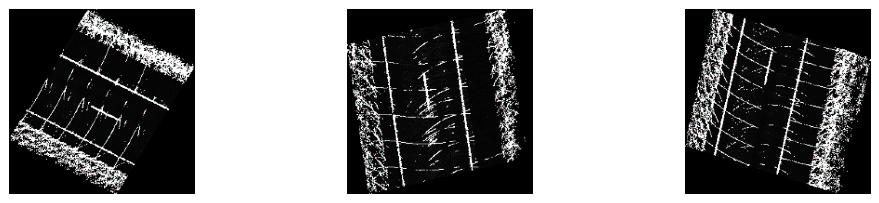
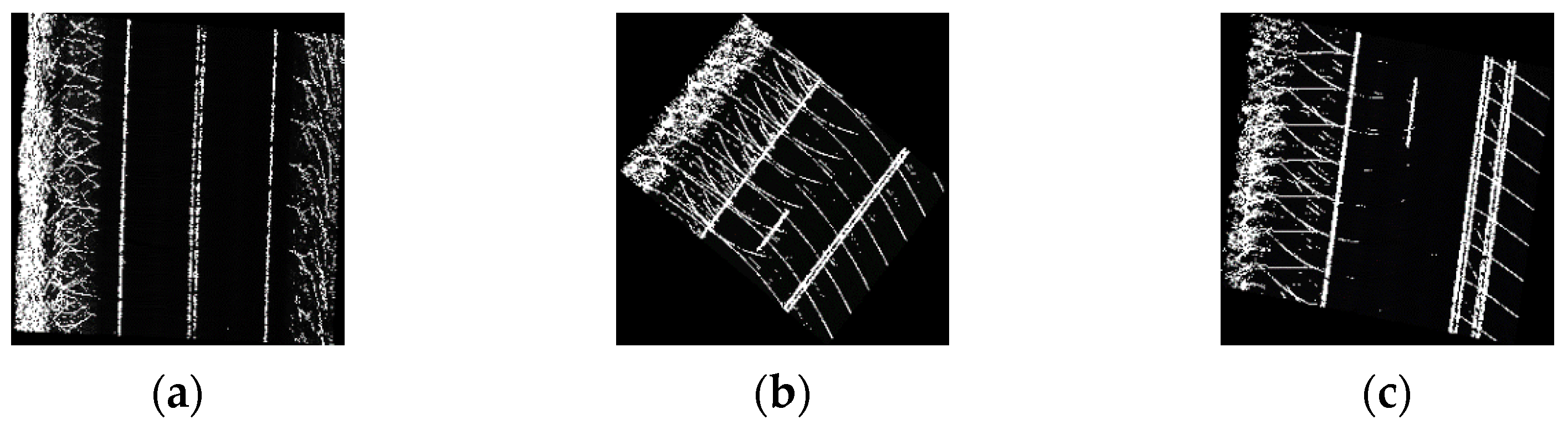
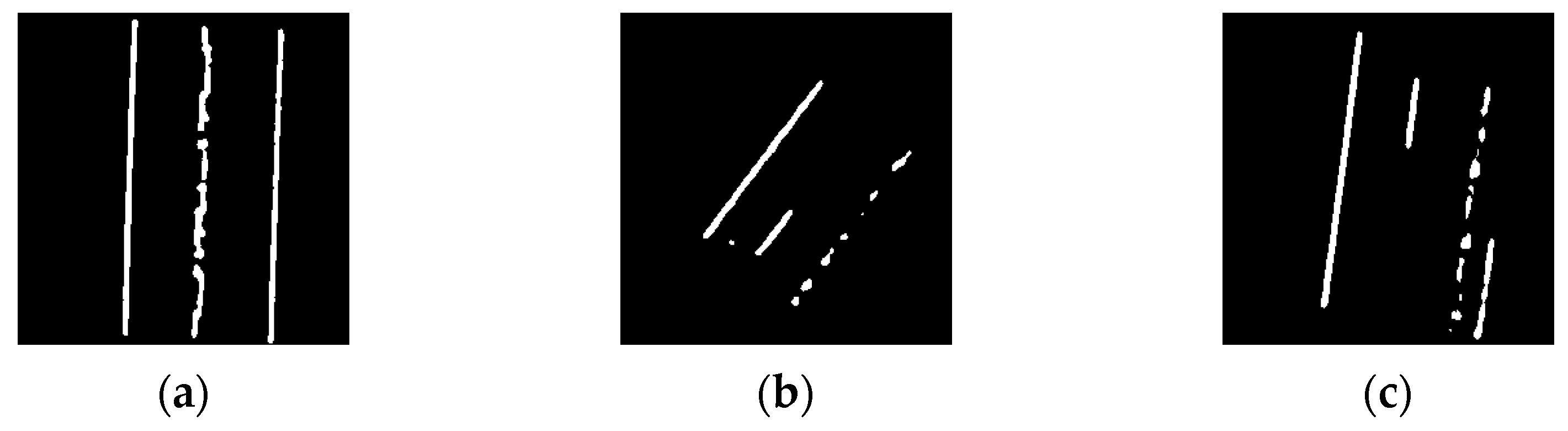
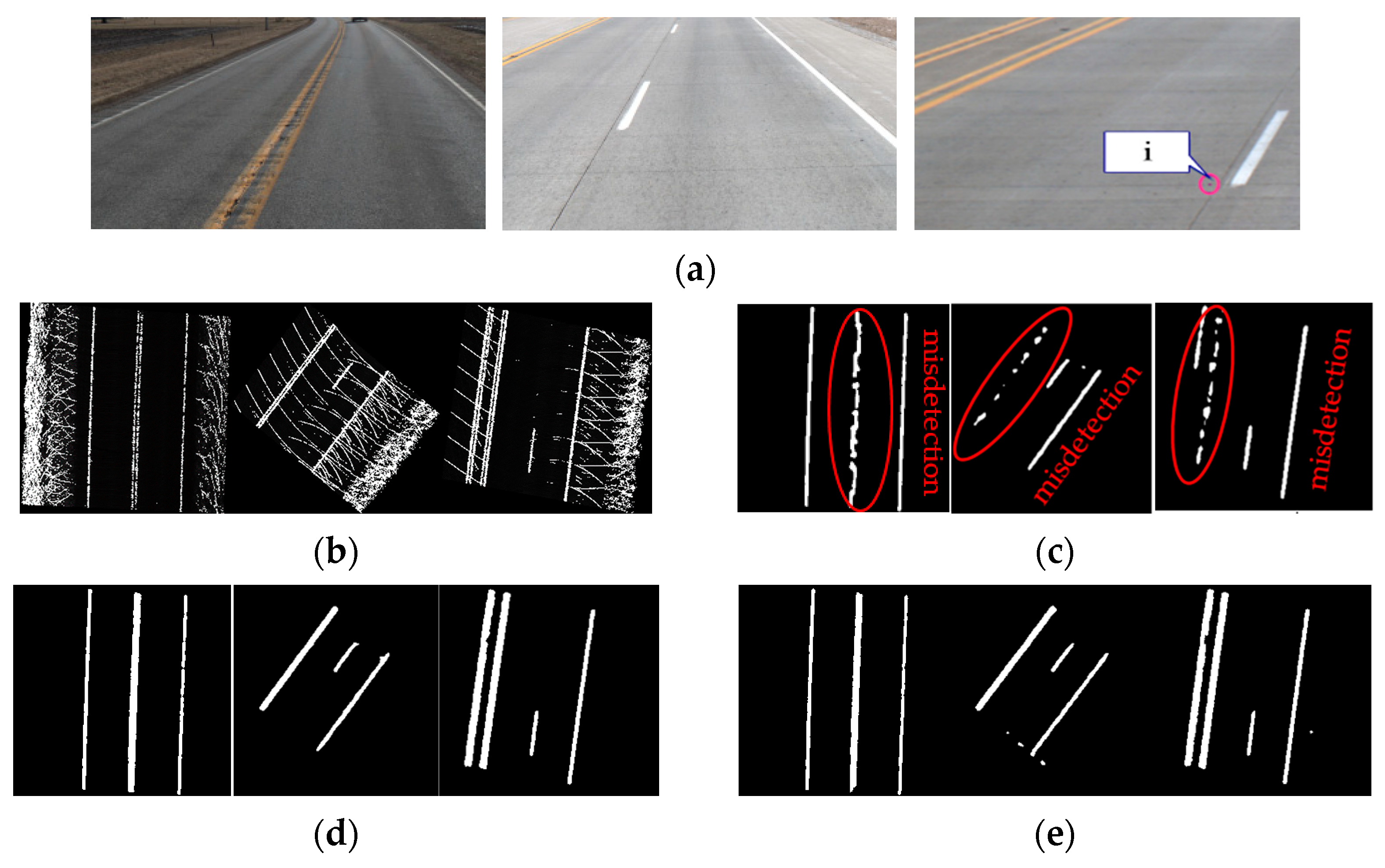
In the previous study [17], a fully convolutional neural network (FCNN), denoted as U-net, was trained for lane marking extraction on two-lane highways. Typical LiDAR intensity images for such regions are shown in Figure 8. The network architecture consisted of two salient paths, as shown in Figure 9—an encoder (on the left in Figure 9) and a decoder (on the right in Figure 9). In this paper, these two paths of the pretrained U-net model were fine-tuned separately to obtain better predictions for different lane marking patterns that were not encountered earlier. As mentioned previously, such new patterns included (a) a one-lane highway with dual lane marking at the center, (b) dual lane markings at the road edge, and (c) a pair of dual lane markings at the road edge; their corresponding LiDAR intensity images are shown in Figure 10. The results of the pretrained model on these new patterns showed significant misdetection, as illustrated in Figure 11.

As per the misdetections in Figure 11, the pretrained model needs to be fine-tuned. One could also argue for training a new model from scratch using LiDAR intensity images with the new lane marking patterns shown in Figure 10. However, since the target domain dataset is small and, thus, less representative of different possible variants of lane marking patterns, this would lead to significant overfitting [34], whereby the model would perform well on new lane marking patterns but obtain poor results in two-lane highway areas. Another overfitting case could also arise if the whole pretrained model was fine-tuned where all network parameters could change to perform well on a small training dataset [35]. Therefore, only the encoder or decoder part of the pre-trained U-net model was fine-tuned in this study.

4. Methodology for U-Net Fine-Tuning and Intensity Profile Generation

The proposed framework for lane marking detection through U-net models and intensity profile generation is illustrated in Figure 12. Road surface blocks were first extracted from LiDAR point clouds. Each block was then rasterized into an intensity image. Furthermore, the training labels are generated automatically [17]. One should note that, since intensity images were directly generated from point clouds, there was no registration error between the point-cloud data and generated intensity images. Encoder/decoder paths of the pretrained U-net were fine-tuned only one at a time to generate two trained models. Hereafter, they are respectively referred to as encoder and decoder-trained U-net models. The individual encoder and decoder training scheme ensured that the network parameters could be adequately adapted to perform well on a new training dataset without overfitting. The performance of fine-tuned models was evaluated on the ground truth generated from both previous and new datasets. Lastly, according to the prediction from the best-performing U-net model, intensity profiles along the road surface were generated and evaluated for discontinuities with the aid of RGB image visualization.

4.1. U-Net Fine-Tuning

For the input data of U-net fine-tuning, this study adopted the strategies proposed by Cheng et al. [17] to generate intensity images and corresponding lane marking labels from LiDAR point clouds. The first step in generating input intensity images was extraction of the road surface point cloud. The extracted point cloud was then tiled at a regular interval of 12.8 m along the driving direction. Hereafter, the 12.8 m long road surface segment is referred to as the “road surface block” (each block typically has 0.4 to 0.8 million points). Here, the width of each road surface block typically ranged between 12 and 16 m. Thus, the interval of 12.8 m ensured minimal resizing along the length and width of the block while generating an image size fixed at 256 × 256 pixels, with a 5 cm cell size. A larger image would increase computations without much improvement in the model, while, with a smaller image, the model would become insensitive to small lane markings that might be rejected as noise. On the other hand, the cell size was chosen on the basis of the average point density which ensured that it was neither too small to result in many empty pixels in the image nor too large such that the level of details in the image was diminished. Furthermore, the typical lane marking width was approximately 6 inches or 15 cm (for both single and dual lane markings) [36] and, thus, the chosen cell size was sufficient for lane marking detection in 3D space as per the masking procedure described in Section 4.2. Once the road surface point cloud was tiled, an intensity enhancement was applied to each road surface block, where intensity values greater than the fifth percentile threshold were set to 255 (LiDAR intensity is recorded as an integer between 0 to 255), while lower ones were maintained. Here, the fifth percentile threshold was based on the assumption that the points with intensity values greater than this threshold were hypothesized lane markings [17], as shown in Figure 13. After that, each road surface block was rasterized into an intensity image. In an intensity image, a pixel value was defined by taking an average of the intensity values of points falling in each cell. A second level of fifth percentile enhancement was then applied to the generated intensity images. The amplification of the high-intensity values, which were hypothesized to originate from lane markings, through the two-step enhancement (for road surface blocks and intensity images) facilitated easier learning for the U-net model.

Once the intensity images were curated for fine-tuning, the next step was to generate the corresponding input lane marking labels. Considering the intensity differences across the used LiDAR scanners on PWMMS-HA, intensity normalization was applied to each road surface block. Then, hypothesized lane marking points were identified from the normalized road surface block using the fifth percentile intensity threshold. The hypothesized lane marking point cloud was further processed for noise removal to extract lane marking points. Interested readers can refer to Cheng et al. [17] for more details about this step. Hereafter, similar to the previously discussed intensity image generation, the lane marking points were rasterized to generate a preliminary labeled image. Lastly, to ensure better spatial structure for the lane markings in the labeled images, a bounding box was defined around each lane marking segment in the preliminary labeled images, and all pixels within the box were labeled as lane marking pixels to generate the final labeled images [17]. Examples of an intensity image and its corresponding labels are shown in Figure 14.

In this study, all differently trained U-net models (including the models used for validating the fine-tuned ones) utilized a loss function based on the dice coefficient for training [37]. For all the models, early stopping criteria were used to stop training when the loss on validation data did not improve for 15 consecutive epochs. The training data were augmented during each epoch through (a) random rotation of the image in a clockwise direction in the range of 0° to 180°, (b) horizontal flipping, and (c) zoom in and out of the image by resizing. An Adam optimizer with a learning rate of $8\times {10}^{-4}$ was used, and it was decayed by a factor of 10 if validation loss did not improve for five consecutive epochs as the training progressed. The performance of all the U-net models was evaluated by reporting metrics such as precision, recall, and F1-score—represented by Equations (1)–(3), where TP, FP, and FN denote true positives, false positives, and false negatives, respectively. TP denotes correct lane marking pixel predictions, FP denotes non-lane marking pixels incorrectly classified as lane marking pixels, and FN denotes lane marking pixels incorrectly classified as non-lane marking pixels. Precision refers to the fraction of accurate lane marking predictions among total lane marking predictions, whereas recall indicates how well the true lane markings were detected. F1-score, which was used to quantify the overall performance, is a harmonic mean of precision and recall.

$$\mathrm{Precision}=\frac{TP}{TP+FP}.$$

(1)

$$\mathrm{Recall}=\frac{TP}{TP+FN}.$$

(2)

$$\mathrm{F}1\text{-}\mathrm{score}=\frac{2\times \mathrm{Precision}\times \mathrm{Recall}}{\mathrm{Precision}+\mathrm{Recall}}.$$

(3)

4.2. Intensity Profiling

Once various U-net models—pretrained, encoder-trained, decoder-trained, and one trained from scratch—were evaluated by the target domain dataset, all the intensity images from the target domain dataset were fed to the best-performing model. The predictions were then used to generate lane marking intensity profiles for reporting intensity information of detected lane markings, as well as investigate the cause behind missing lane markings along transportation corridors. For each intensity image representing a 12.8 m long road surface block, 2D lane marking pixels were predicted by the U-net model. They were then transformed back to 3D for intensity profile generation, whereby intensity values for predicted lane markings were reported along the road surface at regular intervals. The final output was in the form of a plot of intensity value against driving distance along the road.

The centroids derived from the predicted lane marking pixels, as shown in Figure 15a, in an intensity image were regularly spaced at a 5 cm distance, which was the pixel size of the used images. To obtain lane marking predictions with similar point density to the input LiDAR point clouds, we adopted a masking strategy whereby the centroids were utilized to create 2D masks. Around each centroid, a 5 cm square buffer was created along the XY-plane [17]. Neighboring buffer regions were merged to form 2D masks, and each of the merged masks was assigned a mask ID, as shown in Figure 15b.

After that, considering the intensity difference among the different LiDAR units, the hypothesized lane marking point cloud (as mentioned previously, derived from the normalized road surface block by the fifth percentile thresholding) corresponding to each predicted image was utilized. The points in the hypothesized lane marking point cloud falling inside the 2D masks were extracted as final 3D lane marking points and were assigned IDs according to the masks used to extract them, as shown in Figure 15c. There was, however, a caveat to the above-described masking strategy in the case of dual lane marking areas. Since the gap between dual lane markings was 15 cm, which was three times the intensity image resolution, the dual lane markings were predicted as a single marking through the U-net model, as shown in Figure 15d. Thus, only one mask was generated for dual lane markings instead of one mask for each, as displayed in Figure 15e. Through this single mask, the 3D points from both sides of the dual lane marking were grouped as one lane marking segment, as shown in Figure 15f. Only within the regions where the dual lane markings were temporarily separated by a crossing island could the dual lane markings be predicted as two isolated segments. After extracting lane marking segments using all the 2D masks created from intensity images, the derived segments needed to be clustered into the right, middle, and left edges on the basis of road delineation, as shown in Figure 16, for reporting intensity information.

The algorithm used for lane marking segment clustering is graphically depicted in Figure 17. Starting with the extracted lane marking segments within a block, least-squares fitting was applied to each segment for defining the best fitting line, as shown in the zoomed-in cyan rectangle in Figure 17b. Then, two endpoints were defined along the best fitting line of each lane marking segment within two consecutive blocks. Grouping the lane marking in successive blocks depended on the separation between the endpoints of lane marking segments. For endpoints which were more than 40 cm (determined on the basis of the minimum curvature for designing two-lane highways [38]) apart, a given segment would be grouped with another segment in the second block if the angle between a vector joining adjacent endpoints of the two segments (denoted as vector 1 in Figure 17b) and vector along the fitted straight line of the given segment (denoted as vector 2 in Figure 17b) was the smallest among all angles between such segment pairs and did not exceed 8°, which was determined on the basis of the minimum curvature and standard width for designing two-lane highways [38]. Lastly, segments in the two blocks were grouped.

On the other hand, for endpoints which were less than 40 cm apart, vectors 1 and 2 were first defined along the fitted straight line for each segment, as shown in Figure 17c. If the angle between the vectors was less than 8°, the two segments were grouped. These steps were repeated until the lane marking segments from all blocks were processed, as shown in Figure 17d. One should note that, for intersections, the lane marking segments along one direction would be grouped first. The remaining segments would then be grouped by repeating the above steps. Each group of segments was then divided by 2D rectangular buffers with a length of 20 cm along the driving direction and a width of 50 cm (slightly larger than the span of dual lane markings and the gap), as shown in Figure 17e. The final step was to calculate the centroid and average intensity value (from the hypothesized lane marking point clouds) within each buffer to generate intensity profiles along the road. Once the intensity profiles were derived, the locations with lane marking gaps could be identified and investigated further through RGB images to examine their causes, as shown in Figure 18.

5. Results and Discussion

For U-net fine-tuning, an original U-net model, which was trained on two-lane highways (source domain dataset), was fine-tuned to make predictions on datasets with new lane marking patterns such as one-lane highways and dual lane markings at the edge of the road (target domain dataset). Two experiments were conducted: (a) in the first, only encoder weights could change; (b) in the second, only decoder weights could change. Another experiment was also conducted where another U-net model was trained from scratch on both source and target domain datasets. The performance comparison of this model with fine-tuned models helped in analyzing the effectiveness of transfer learning for lane marking extraction in new patterns. Additionally, both encoder- and decoder-trained U-net models were also evaluated using the past test dataset to assess if fine-tuning negatively affected their performance on two-lane highways due to overfitting to new lane marking patterns. Furthermore, all four U-net models were evaluated on the independent test dataset (not belonging to either source or target domain dataset locations) to obtain another assessment of their generalization capability. Once the U-net models were evaluated on various test datasets, all the intensity images (4682 images) from the target domain dataset were fed to the best-performing model for intensity profile generation. The description of used datasets for training or fine-tuning, validation, testing, and intensity profile generation are summarized in

Table 1. Datasets used for training or fine-tuning, validation, testing, and intensity profile generation of various U-net models.

U-Net Model	Pairs of Intensity and Labeled Images (Training or Fine-Tuning)/(Validation)	Intensity Images for Testing
Pretrained	Source domain dataset 1: 1183/238 pairs	Source domain dataset 1: 174 intensity images Target domain dataset 2: 122 intensity images Independent dataset 3: 100 intensity images
Encoder-trained	Target domain dataset 2: 267/69 pairs
Decoder-trained	Target domain dataset 2: 267/69 pairs
Trained from scratch	Combined source and target dataset: 1450 (1183 1 + 267 2)/307 (238 1 + 69 2) pairs
U-Net Model	Intensity Images for Intensity Profile Generation
Encoder-trained (best-performing)	Whole target domain dataset 3: 4682 intensity images

¹ Two-lane highway patterns; ² one-lane highway patterns; ³ one- and two-lane highway patterns.

. The model fine-tuning/training was executed on the Google Collaboratory platform that provides free K-80 GPU access. The Keras deep learning framework was used to implement U-net.

Table 2. Time taken by various steps in the proposed strategy for intensity image generation, U-net training, and intensity profile generation.

Step	Time Taken (min)	Platform
Intensity image generation (per mile)	~5	32 GB RAM computer
Pretrained U-net model (1183 images)	~60	Google Collaboratory
Training fine-tuned U-net models (346 images) 1	~15	Google Collaboratory
Training U-net model from scratch (1450 images)	~75	Google Collaboratory
Intensity profiling (per mile)	~10	32 GB RAM computer

¹ Almost the same for encoder and decoder.

lists the time taken by each step in the adopted methodology.

In this study, 1421 pairs (1183 for training and 238 for validation) of intensity image and corresponding label from the source domain dataset were used, while, for the target domain dataset, a total of 336 such pairs were generated. Both encoder- and decoder-trained U-net models utilized 267 images for training and the remaining 69 images for validation. The model trained from scratch used 1450 (1183 + 267) and 307 (238 + 69) images for training and validation, respectively. For testing, lane marking extraction results from the target domain dataset (122 intensity images) for various U-net models—pretrained, encoder-trained, decoder-trained, and one trained from scratch—are presented in

Table 3. Performance metrics of various U-net models on new test dataset (target domain ¹).

Model	Precision (%)	Recall (%)	F1-Score (%)
Pretrained U-net	84.6	58.4	65.7
Encoder-trained U-net 2	86.4	88.1	86.9
Decoder-trained U-net	83.9	83.1	82.1
U-net model trained from scratch	83.9	72.2	75.2

¹ One-lane highway patterns (174 intensity images); ² the model with the best performance.

. Additionally, to gauge the generalization ability of newly trained models (fine-tuned and trained from scratch), they were also evaluated on source domain datasets (174 intensity images), and their performance was compared with the pretrained one, as listed in

Table 4. Performance metrics of various U-net models on past test dataset (source domain ¹).

Model	Precision (%)	Recall (%)	F1-Score (%)
Pretrained U-net	84.1	87.9	85.9
Encoder-trained U-net 2	81.8	87.9	84.7
Decoder-trained U-net	72.6	87.5	79.4
U-net model trained from scratch	79.0	87.2	82.9

¹ Two-lane highway patterns (122 intensity images); ² the model with the best performance.

. Lastly, performance measures on independent test data (100 intensity images) are provided in

Table 5. Performance metrics of various U-net models on independent test dataset ¹.

Model	Precision (%)	Recall (%)	F1-Score (%)
Pretrained U-net	89.8	83.9	86.3
Encoder-trained U-net 2	90.7	90.3	90.1
Decoder-trained U-net	82.5	85.8	83.2
U-net model trained from scratch	81.1	85.8	82.5

¹ One- and two-lane highway patterns (100 intensity images); ² the model with the best performance.

.

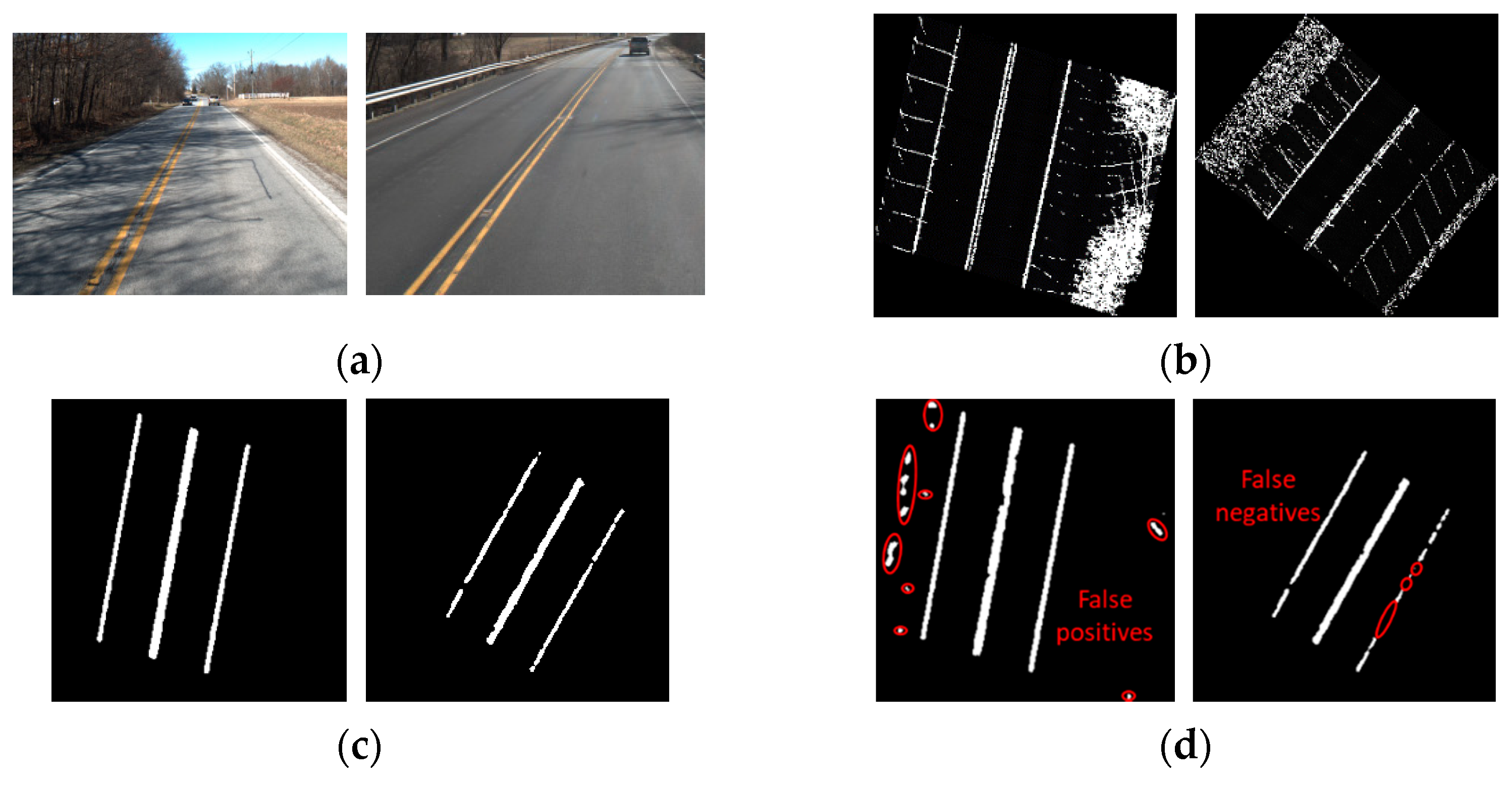
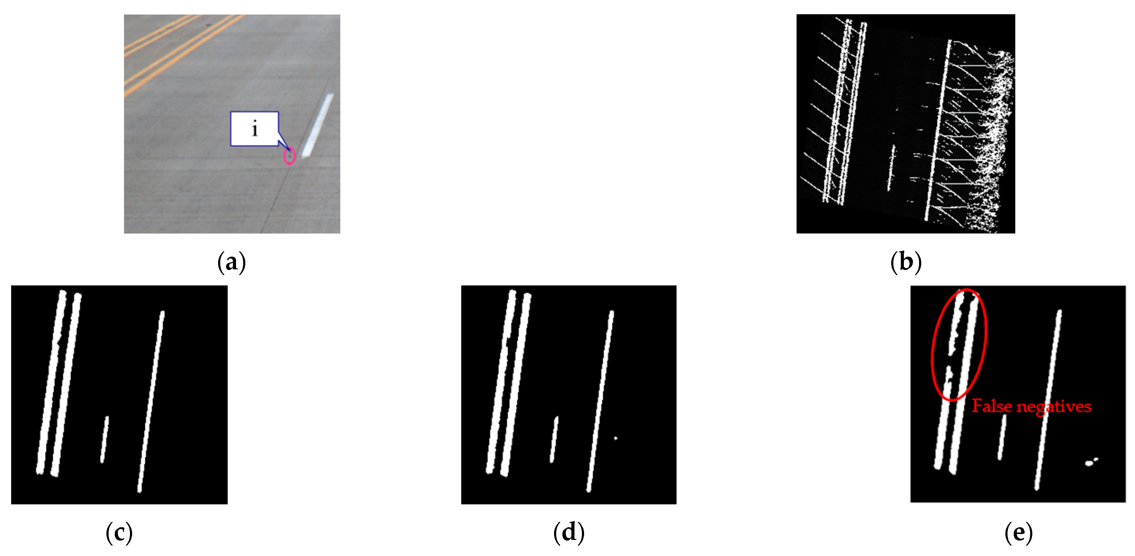
As evident from Table 3, the pretrained model showed substandard performance on the new test dataset with an F1-score of only 65.7%, which was due to poor predictions in new lane marking patterns. On the other hand, the encoder- and decoder-trained models obtained better F1-scores of 86.9% and 82.1%, respectively. Figure 19 shows the superior performance of fine-tuned models over the pretrained one, whereby the latter showed misdetection in areas with new lane marking patterns. Furthermore, the encoder-trained model performed better than the decoder-trained one as evident by the respective F1-score values. Specifically, the former was able to eliminate false positives and false negatives to a larger extent than the latter, as illustrated in Figure 20.

The better performance of the encoder-trained model is owed to the fact that, in deep learning models, the shallow layers (the encoder path) learn low-level features [27]. In the context of lane marking extraction, such features include speckle pattern and distribution of high-intensity non-lane marking points, which vary from dataset to dataset depending upon lane marking patterns and are critical for accurate prediction. While freezing the encoder and training decoder, we did not allow the network to learn such low-level features in the new training dataset leading to worse performance. Lastly, the model trained from scratch, while performing better than the pretrained model, was outperformed by both fine-tuned models, as evident by the F1-scores in Table 3. The inferior performance of the model trained from scratch compared to fine-tuned models was expected since the combined training dataset was still dominated by previous lane marking samples, and the number of new training samples was not enough to adapt network parameters for better performance in new lane marking patterns. This is visualized in Figure 21 where the model trained from scratch showed partial detections in areas with pair of dual lane markings at the edge. In addition, another demerit of the model trained from scratch was its fivefold longer training time compared to fine-tuning, as mentioned in Table 2. A large number of training samples and random initial weights (no prior knowledge embedded) increased the training time.

As far as the performance on the source domain dataset is concerned, the encoder-trained model with F1-score of 84.7% again outperformed the decoder trained one with an F1-score of just 79.4% and the model trained from scratch with an F1-score of 82.9%, as listed in Table 4. In addition, the encoder-trained model’s performance was comparable to the pretrained U-net model (F1-score 85.9%), which shows that the encoder-trained model generalized well on the source domain dataset in addition to robust predictions on the target domain dataset. Lastly, as can be seen from Table 5, once again, the encoder-trained model outperformed all other models with an F1-score of 90.1%. In summary, the encoder-trained U-net model obtained by fine-tuning a pretrained model with only a few hundred images not only performed better on the target domain test dataset but also generalized well to the source domain and independent test datasets.

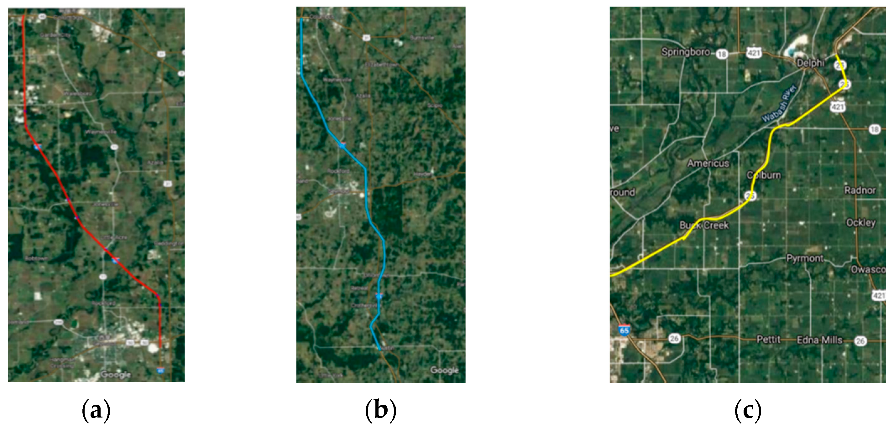
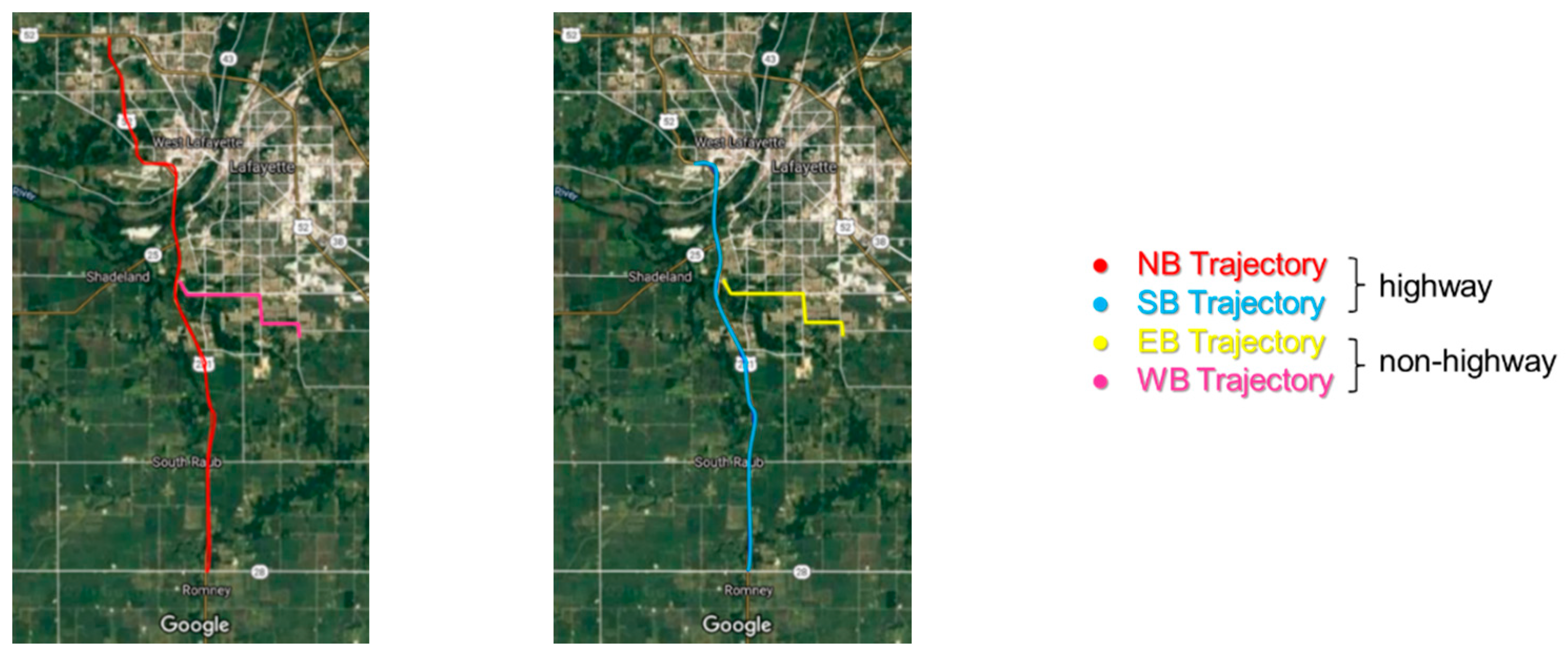
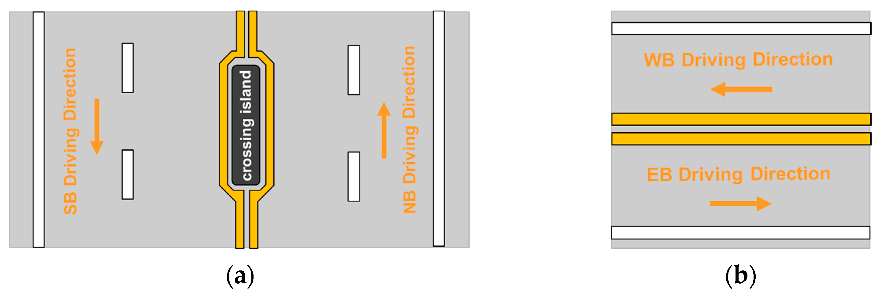
The intensity profiles for lane marking predictions by the encoder-trained U-net (the best-performing model) in the whole target domain dataset (a total of 4682 intensity images for NB, SB, WB, and EB segments) were derived for the right, middle, and left edges of the roadway. 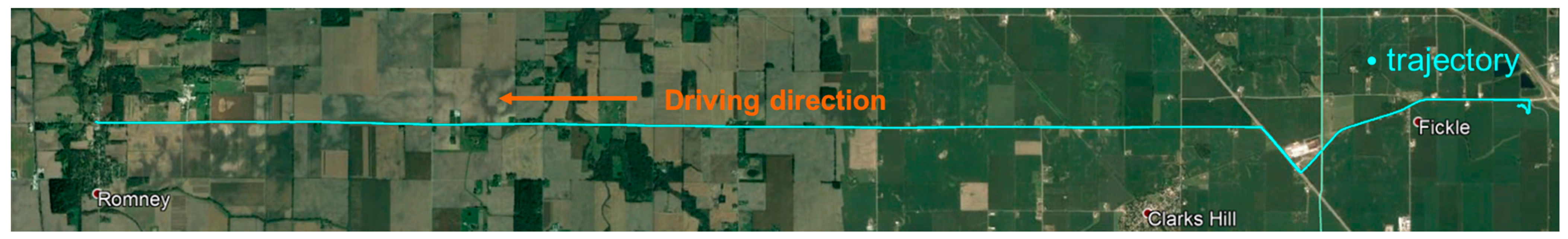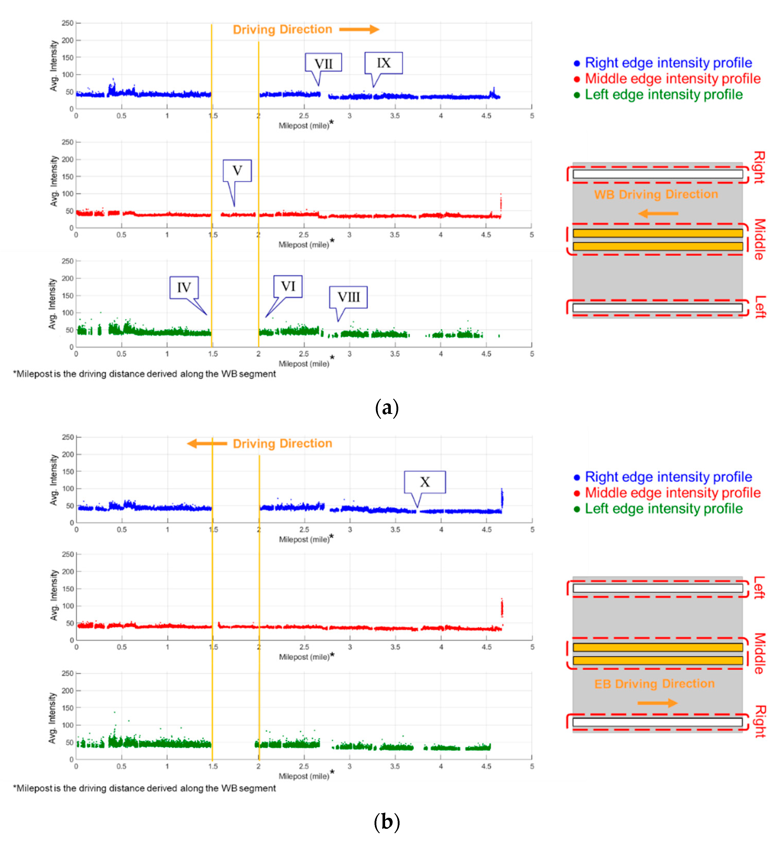The NB and SB segments were surveyed on the outer lane of a two-lane highway whose common lane markings were center dual yellow lines, as shown in Figure 22a. Hence, only the left-edge profiles from NB and SB segments corresponded (note: in some regions, the dual lane markings were temporarily separated by a crossing island). On the other hand, WB and EB segments were collected in opposite driving directions, as shown in Figure 22b, on the same rural road divided by the center dual yellow lines. The intensity profiles derived from the WB segment could be related to those from the EB segment. For example, the right-edge profile from the WB segment could correspond to the left-edge profile from EB segment. For NB and SB segments, the intensity profiles and the corresponding RGB images are visualized in Figure 23 and Figure 24, while those for WB and EB segments are displayed in Figure 25 and Figure 26.

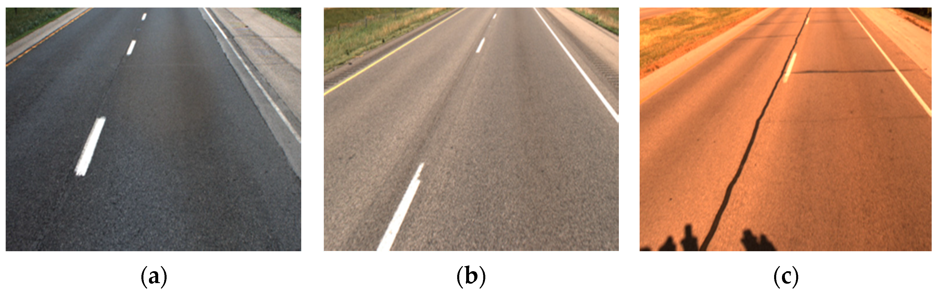
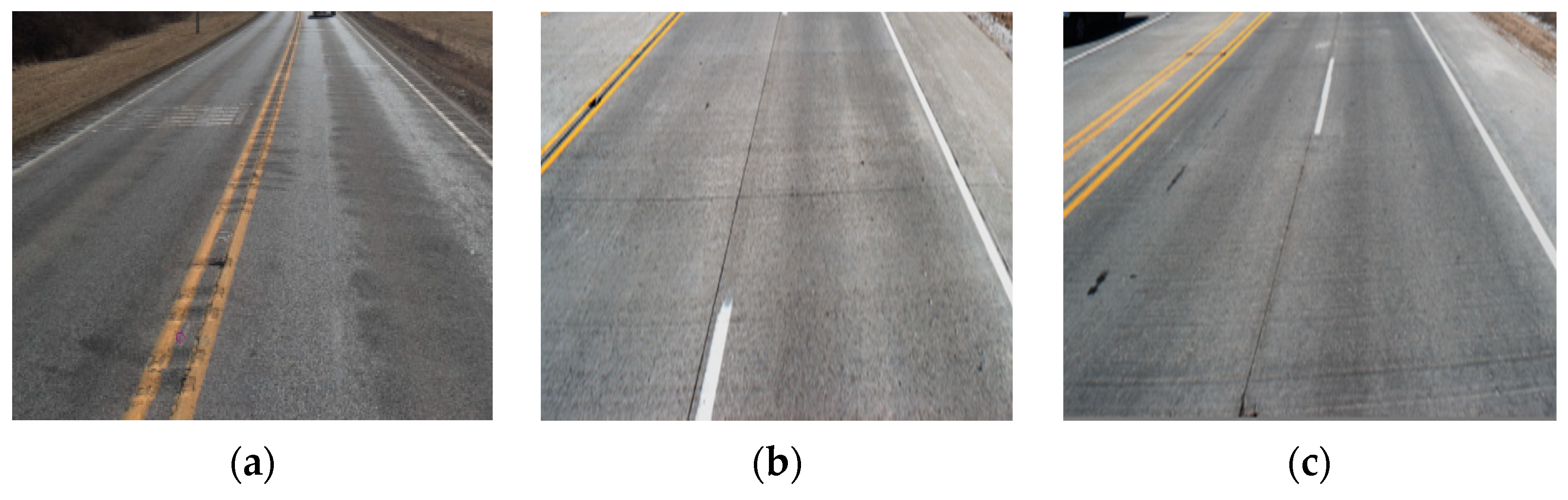
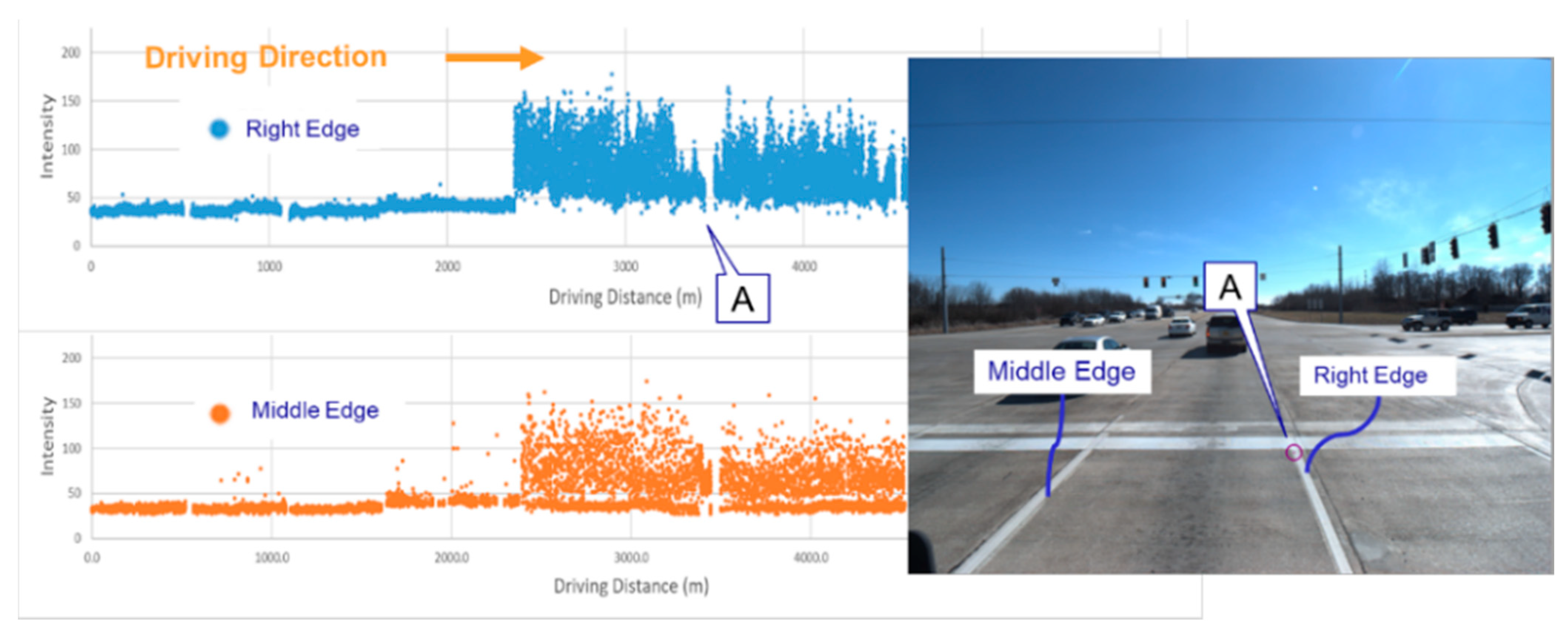
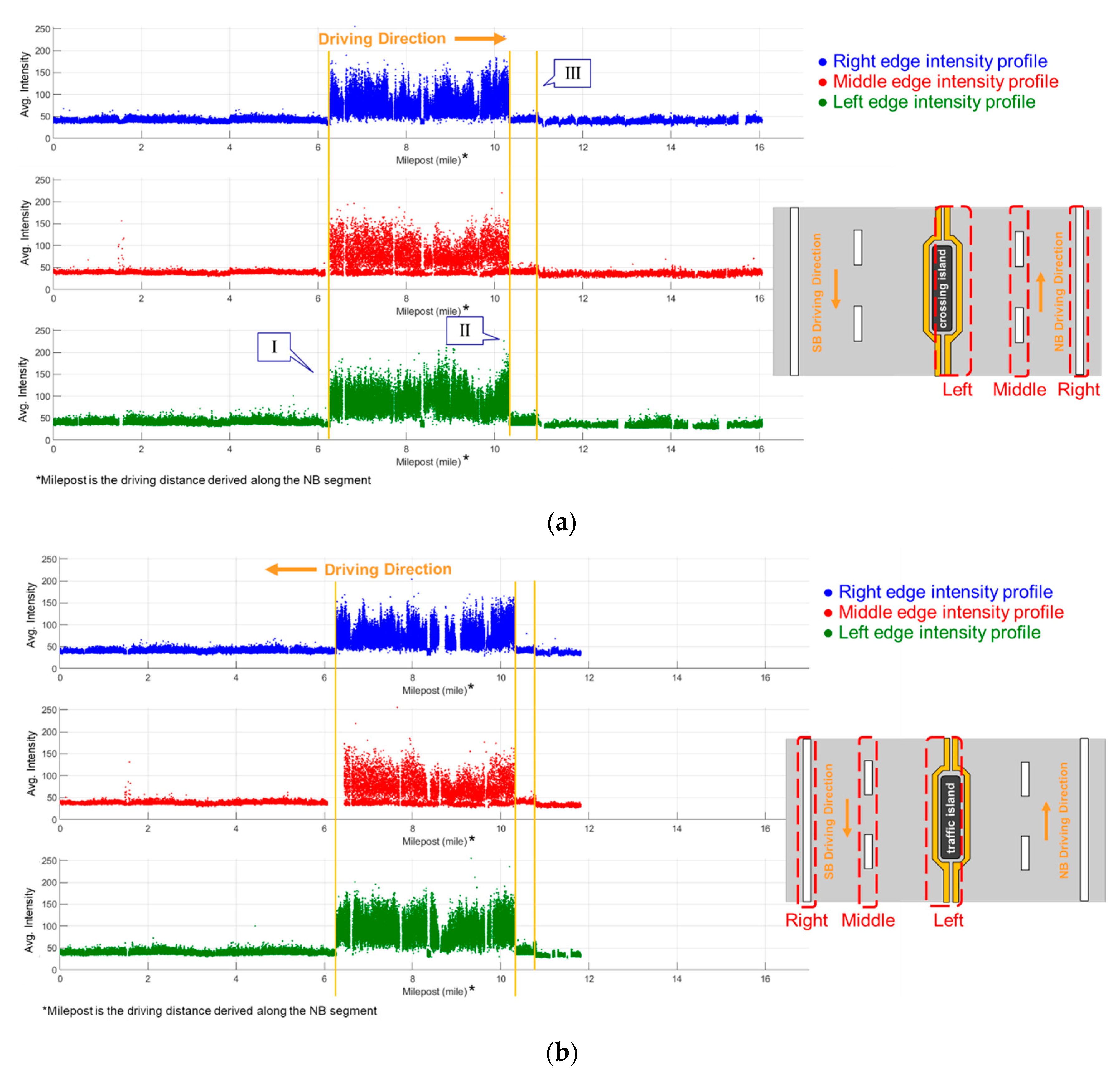
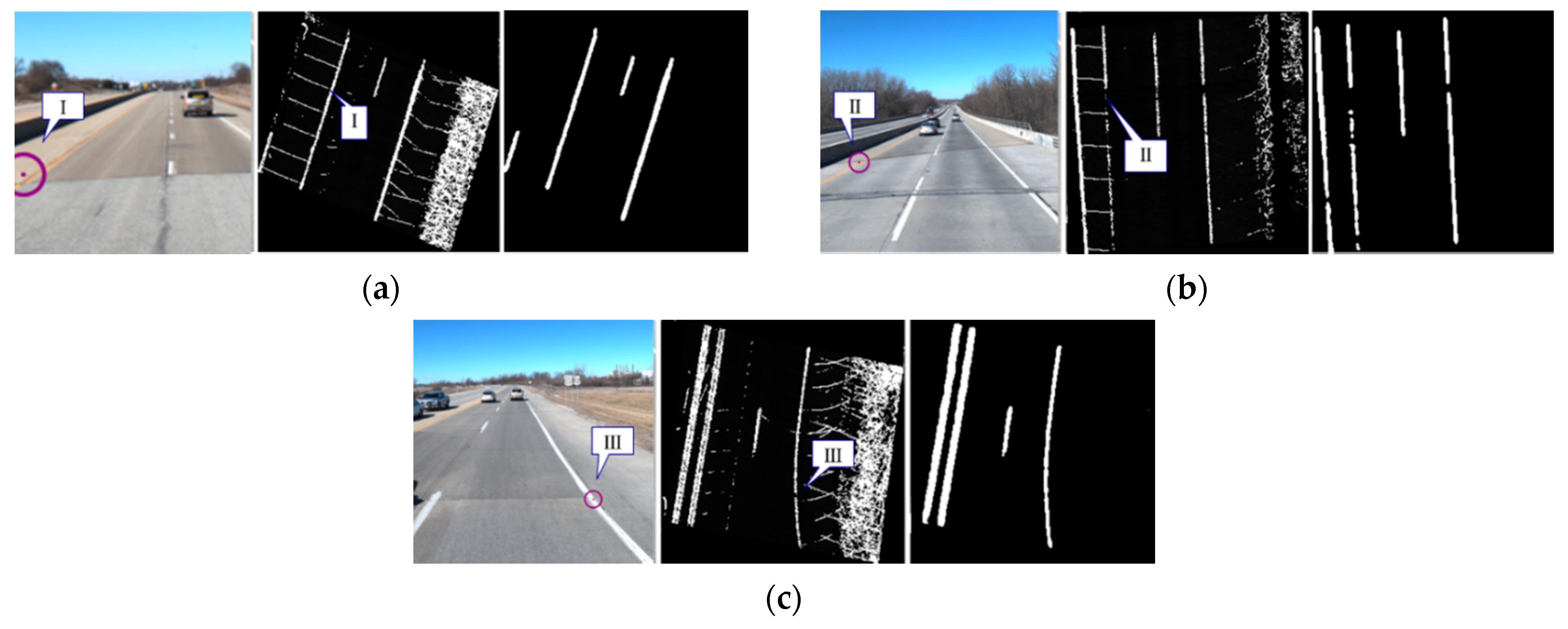
Using the corresponding nature of profiles in different dataset segments, the repeatability of the proposed strategies for detecting lane markings and generating intensity profiles could be demonstrated. As can be seen in Figure 23a,b, sudden intensity changes in the profiles for both NB and SB segments could be observed at locations I, II, and III within milepost range 6–10. The cause behind these sudden intensity changes was a transition of pavement from asphalt to concrete, shown in Figure 24a,b, where it is known that the average luminance of concrete pavements is 1.77 times that of asphalt pavements [39]. Another area with different asphalt pavements can be seen in Figure 24c. Next, as displayed in Figure 25, the right-, middle-, and left-edge intensity profiles from the WB segment were almost the same as the left, middle, and right ones, respectively, from the EB segment. At locations IV, V, and VI in Figure 25, the missing lane marking regions could be identified and visualized through the corresponding images, as shown in Figure 26a–c. A roundabout and its merging region led to the long gap for locations IV, V, and VI in Figure 25.

Furthermore, the agreement of intensity profiles derived from NB/SB and WB/EB segments was estimated by comparing the average intensity values at the same location.

Table 6. Intensity profile difference statistics for NB and SB segments (common lane markings, length: 9.7 miles).

Statistic	(SB_Left) − (NB_Left)
Mean	−0.95
STD	3.01
RMSE	3.16

and

Table 7. Intensity profile difference statistics for WB and EB segments (length: 4.6 miles).

Statistic	(EB_Left) − (WB_Right)	(EB_Mid) − (WB_Mid)	(EB_Right) − (WB_Left)
Mean	−0.24	0.23	0.81
STD	4.36	2.43	4.14
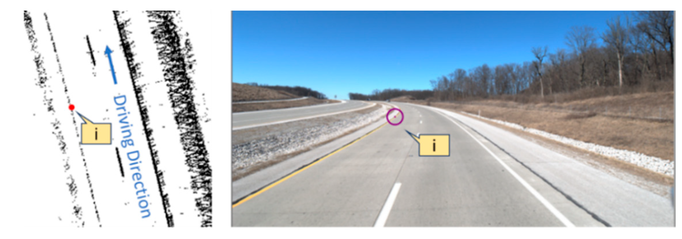
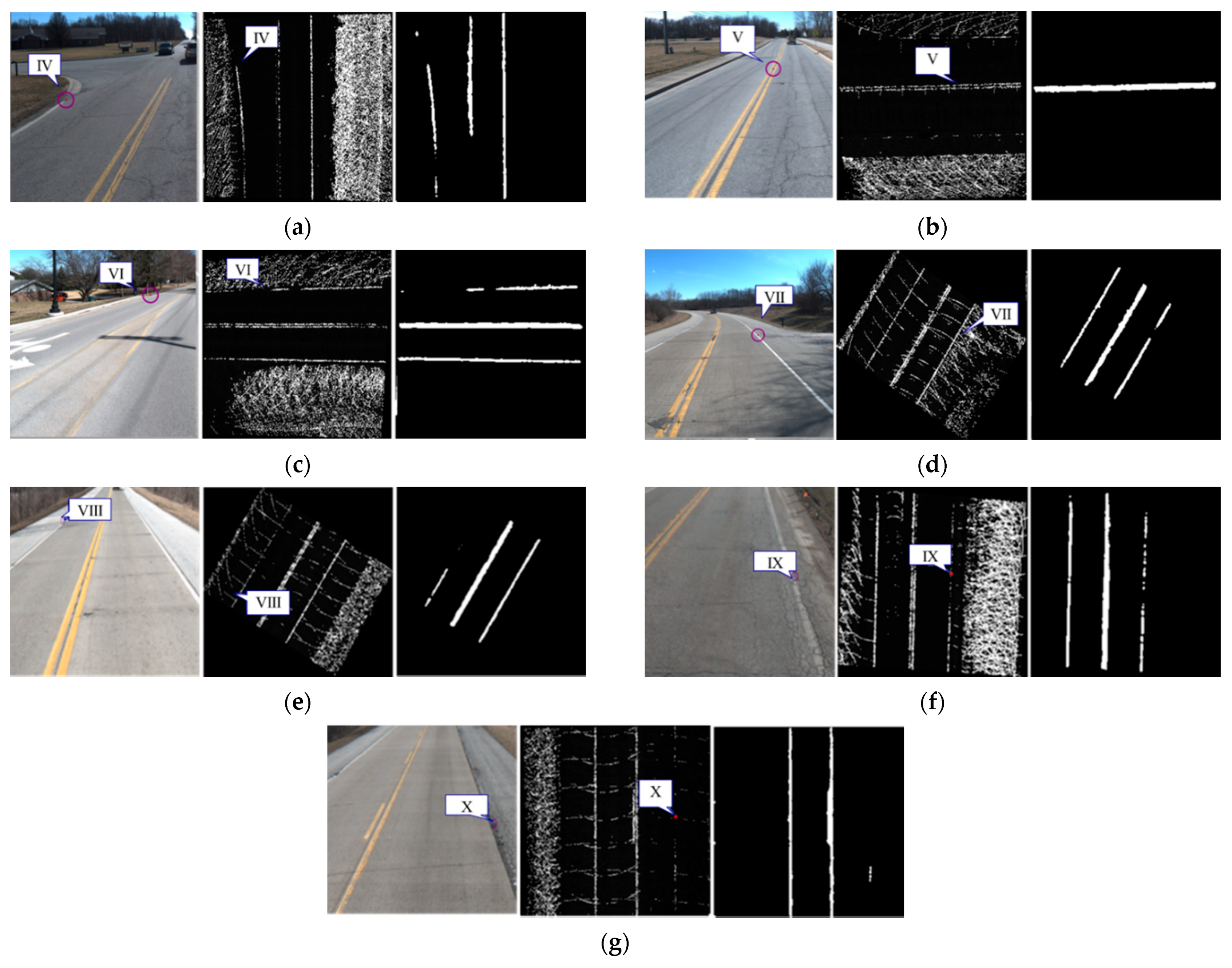
RMSE	4.37	2.44	4.22

list the difference statistics for the intensity profiles from NB/SB and WB/EB segments, respectively. The results show that the root-mean-squared error (RMSE) of the NB/SB intensity profiles (left-edge common lane markings) was around 3.2 (note: PWMMS-HA provided intensity as an integer number within 0–255). The average intensity values from WB and EB segments (three edges lane markings) were in agreement within the range of 4.2 to 4.4. Lastly, RGB image visualization identified the following four primary causes behind the intensity profile gaps: (a) misdetection by the U-net model in spite of high intensity of lane marking points, (b) adequately visible lane markings in RGB images but not reflective enough to be detected as high-intensity points in LiDAR point cloud, (c) worn-out lane markings leading to poor reflectivity, and (d) absence of lane markings. An example location for each of the above conditions is marked in the intensity profiles in Figure 25 (locations VII, VIII, IX, and X), and they are further illustrated in Figure 26c–f by the RGB images, intensity image, and lane marking predictions by the encoder-trained U-net model. One should note that the datasets used for intensity profile generation were collected on highway and non-highway regions at different speed limits (25–60 mph), which resulted in road surface blocks with varying point density (ranging from 2500 to 7500 points per m²). Accurate lane predictions, as shown in Figure 24 (highway region) and Figure 26 (non-highway region), prove that the lane marking extraction by the U-net model was agnostic to point density.

6. Conclusions and Recommendations for Future Research

Recently, lane marking extraction from LiDAR data using deep learning has gained impetus. However, the requirement of a large number of training samples, which are usually generated manually, is a major bottleneck. Efforts have been made to automate the labeling of intensity images for lane marking extraction; however, curating a new training dataset with many samples for every LiDAR data collection by a different scanner or at different locations with new lane marking patterns is not practical. Hence, this paper presented a transfer learning approach of domain adaptation whereby a U-net model trained on an earlier LiDAR dataset (source domain data collected on two-lane highways) was fine-tuned to make lane marking predictions on another dataset with new lane marking patterns (target domain data collected over one-lane highways, with dual lane markings at the center, and with a pair of dual lane markings at the edge). With this approach, a robust U-net model was trained using only a few training examples from the target domain dataset. To this end, two U-net models were established after fine-tuning either the encoder or decoder path of a pretrained U-net model referred to as encoder-trained and decoder-trained U-net, respectively. Additionally, another U-net model was trained from scratch on combined source and target domain datasets to analyze the benefits of fine-tuning.

On the target domain dataset, the encoder-trained U-net performed the best with an F1-score of 86.9%, while the decoder-trained U-net showed an F-score of 82.1%. Furthermore, the model trained on combined datasets achieved an F1-score of only 75.2% and took nearly fivefold longer to train than the fine-tuned models as a result of a larger training dataset and random initial weights. The fine-tuned models, on the other hand, were trained on a small dataset with initial weights derived from the pretrained model.

On the source dataset, the encoder-trained model obtained an F1-score of 84.7%, while the same metric for the decoder-trained model was 79.4%. The model trained from scratch obtained an F1-score of 82.9%, performing better than the decoder-trained model but not the encoder-trained one. Furthermore, the pretrained model had an F1-score of 85.9% on the same dataset, which was reasonably matched by the encoder-trained model. Additionally, an independent test dataset belonging to neither source nor domain dataset locations was curated to further evaluate the U-net models, where the encoder-trained model outperformed all the other ones with an F1-score of 90.1%. The aforementioned performance results on the target domain, source domain, and independent dataset lead to two conclusions. First, when the target domain dataset is small and different from the source domain dataset, it is preferable to fine-tune a pretrained model than train a model from scratch on combined source and target domain datasets. Secondly, it is preferable to fine-tune encoder weights than decoder ones in a U-net during domain adaptation.

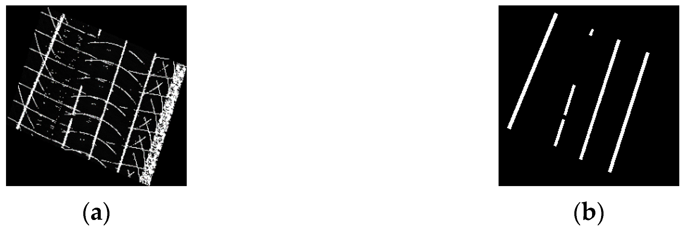
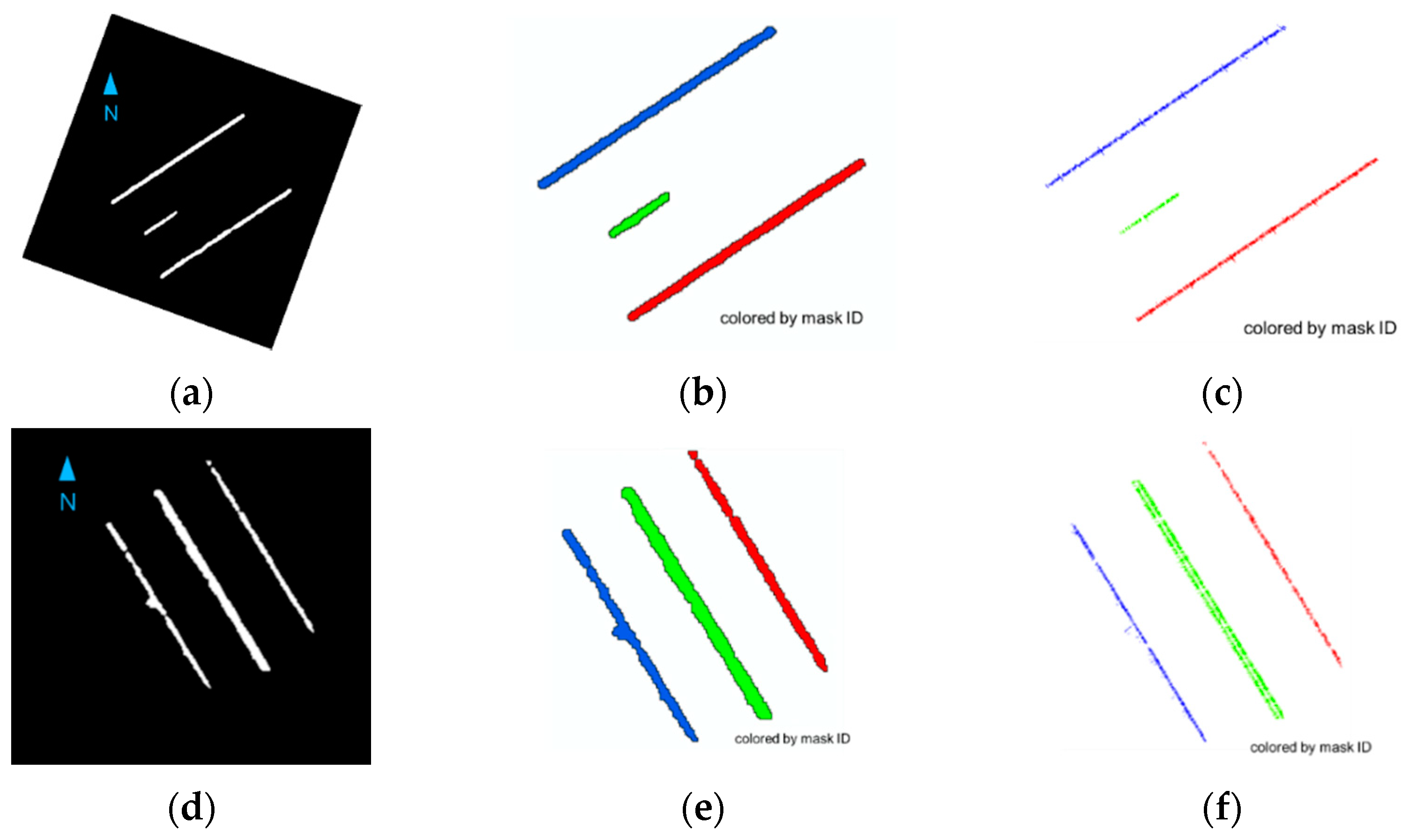
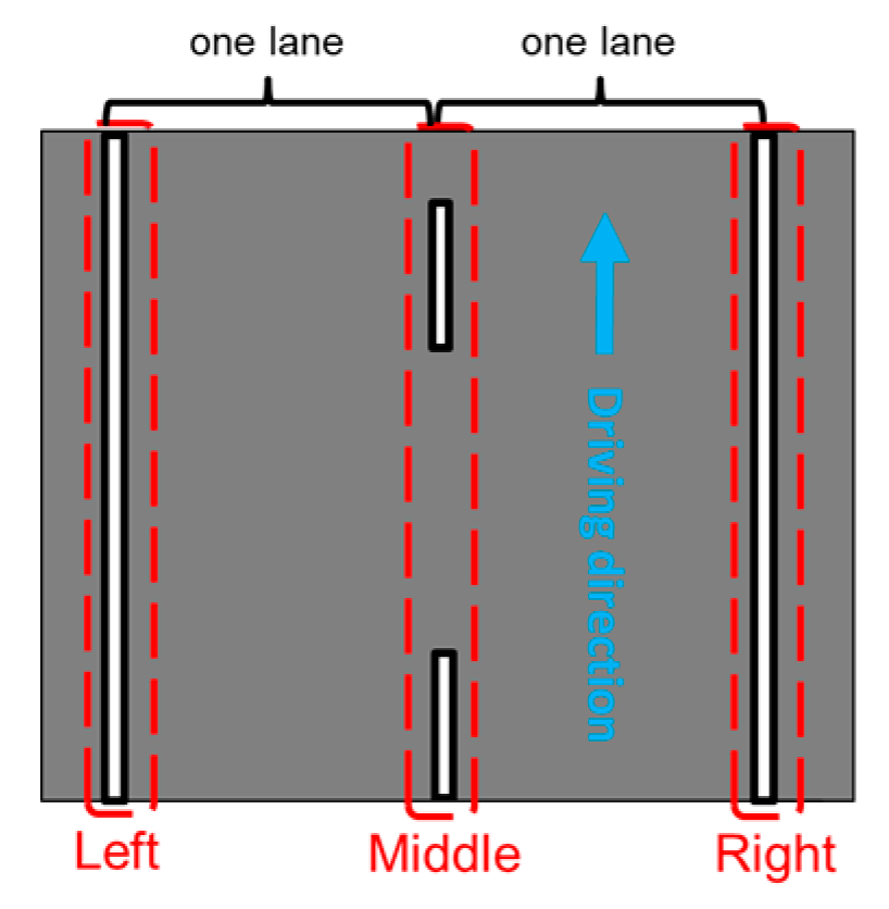
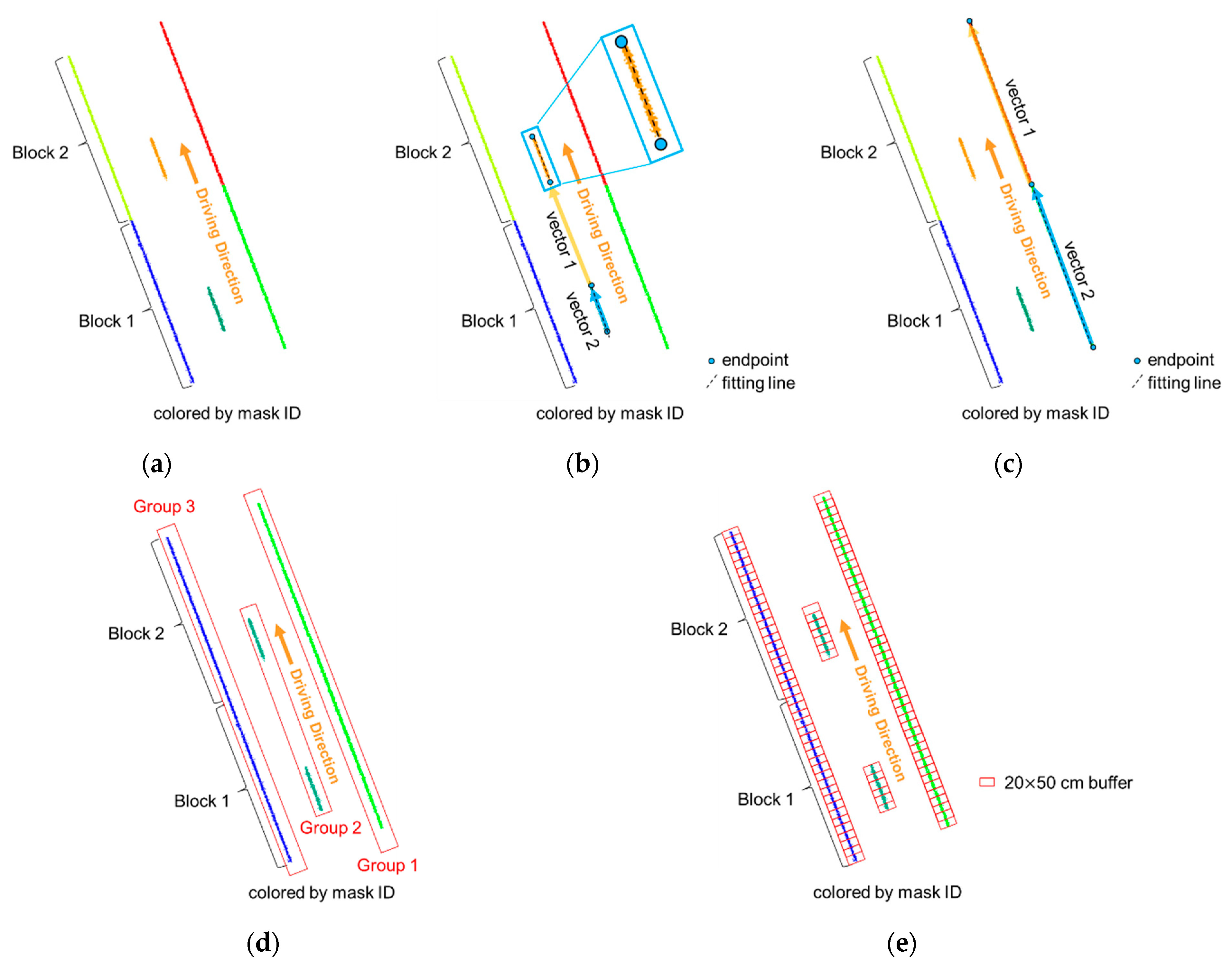
The second part of this paper proposed an intensity profile generation strategy, whereby lane marking intensity variation along the driving direction was reported at regular intervals. First, 3D LiDAR points were extracted by 2D masks generated using the lane marking pixels predicted from the best-performing U-net model (encoder-trained). The extracted lane markings were then clustered into right, middle, and left edges according to the road delineation. Along the driving direction, each group of extracted lane markings was divided by 2D rectangular buffers to estimate the average intensity of the points falling in each buffer. Lastly, the average intensity versus the driving distance (intensity profile) for each edge lane marking was depicted.

For the repeatedly surveyed lane markings, the intensity differences across the derived profiles were within the range of 4.2 to 4.4 (with intensity values registered as integer values within 0 to 255 range), which demonstrated the robustness of the proposed strategies for detecting lane markings and generating intensity profiles. Another benefit of the proposed strategy is the identification of regions with sudden intensity changes due to transition from one pavement type to another, verified by RGB imagery visualization. Moreover, intensity profiling coupled with RGB image visualization can assist departments of transportation in improving and maintaining lane markings while significantly reducing manual labor and mitigating risk associated with in-person inspection.

In the current approach, the proposed strategy cannot predict lane markings in real time. A major bottleneck is the sequential generation of intensity images from road surface point-cloud block, which will be addressed in the future by parallelizing this procedure. Another avenue for future work is testing the encoder-trained U-net model on datasets acquired by different LiDAR units of different models and gauging how well it can generalize. Moreover, in the misdetection regions where lane markings can be observed by the coacquired images, the color and texture information of these images can be utilized to identify undetected points from LiDAR datasets. Through this image-based refinement, the performance of lane marking extraction can be improved.

References

1. Seif, H.G.; Hu, X. Autonomous driving in the iCity—HD maps as a key challenge of the automotive industry. Engineering 2016, 2, 159–162. [Google Scholar] [CrossRef] [Green Version]
2. Smadi, O.; Souleyrette, R.R.; Ormand, D.J.; Hawkins, N. Pavement marking retroreflectivity: Analysis of safety effectiveness. Transp. Res. Rec. 2008, 2056, 17–24. [Google Scholar] [CrossRef]
3. Carnaby, B. Poor road markings contribute to crash rates. In Proceedings of the Australasian Road Safety Research Policing Education Conference, Wellington, New Zealand, 14–16 November 2005. [Google Scholar]
4. Ghallabi, F.; Nashashibi, F.; El-Haj-Shhade, G.; Mittet, M.-A. Lidar-based lane marking detection for vehicle positioning in an hd map. In Proceedings of the 2018 21st International Conference on Intelligent Transportation Systems (ITSC), Maui, HI, USA, 4–7 November 2018. [Google Scholar]
5. Guan, H.; Li, J.; Yu, Y.; Wang, C.; Chapman, M.; Yang, B. Using mobile laser scanning data for automated extraction of road markings. ISPRS J. Photogramm. Remote Sens. 2014, 87, 93–107. [Google Scholar] [CrossRef]
6. Jung, J.; Che, E.; Olsen, M.; Parrish, C. Efficient and robust lane marking extraction from mobile lidar point clouds. ISPRS J. Photogramm. Remote Sens. 2019, 147, 1–18. [Google Scholar] [CrossRef]
7. Yu, Y.; Li, J.; Guan, H.; Jia, F.; Wang, C. Learning hierarchical features for automated extraction of road markings from 3-D mobile LiDAR point clouds. IEEE J. Sel. Top. Appl. Earth Obs. Remote Sens. 2014, 8, 709–726. [Google Scholar] [CrossRef]
8. Yan, L.; Liu, H.; Tan, J.; Li, Z.; Xie, H.; Chen, C. Scan line based road marking extraction from mobile LiDAR point clouds. Sensors 2016, 16, 903. [Google Scholar] [CrossRef] [PubMed]
9. Kashani, A.G.; Olsen, M.J.; Parrish, C.E.; Wilson, N. A review of LiDAR radiometric processing: From ad hoc intensity correction to rigorous radiometric calibration. Sensors 2015, 15, 28099–28128. [Google Scholar] [CrossRef] [Green Version]
10. Höfle, B.; Pfeifer, N. Correction of laser scanning intensity data: Data and model-driven approaches. ISPRS J. Photogramm. Remote Sens. 2007, 62, 415–433. [Google Scholar] [CrossRef]
11. Tan, K.; Cheng, X.; Ding, X.; Zhang, Q. Intensity data correction for the distance effect in terrestrial laser scanners. IEEE J. Sel. Top. Appl. Earth Obs. Remote Sens. 2015, 9, 304–312. [Google Scholar] [CrossRef]
12. Krooks, A.; Kaasalainen, S.; Hakala, T.; Nevalainen, O. Correction of intensity incidence angle effect in terrestrial laser scanning. ISPRS Ann. Photogramm. Remote Sens. Spat. Inf. Sci. 2013, 2, 145–150. [Google Scholar] [CrossRef] [Green Version]
13. Bolkas, D. Terrestrial laser scanner intensity correction for the incidence angle effect on surfaces with different colours and sheens. Int. J. Remote Sens. 2019, 40, 7169–7189. [Google Scholar] [CrossRef]
14. Torrance, K.E.; Sparrow, E.M. Theory for off-specular reflection from roughened surfaces. J. Opt. Soc. Am. 1967, 57, 1105–1114. [Google Scholar] [CrossRef]
15. He, B.; Ai, R.; Yan, Y.; Lang, X. Lane marking detection based on convolution neural network from point clouds. In Proceedings of the 2016 IEEE 19th International Conference on Intelligent Transportation Systems (ITSC), Rio de Janeiro, Brazil, 1–4 November 2016. [Google Scholar]
16. Wen, C.; Sun, X.; Li, J.; Wang, C.; Guo, Y.; Habib, A. A deep learning framework for road marking extraction, classification and completion from mobile laser scanning point clouds. ISPRS J. Photogramm. Remote Sens. 2019, 147, 178–192. [Google Scholar] [CrossRef]
17. Cheng, Y.-T.; Patel, A.; Wen, C.; Bullock, D.; Habib, A. Intensity Thresholding and Deep Learning Based Lane Marking Extraction and Lane Width Estimation from Mobile Light Detection and Ranging (LiDAR) Point Clouds. Remote Sens. 2020, 12, 1379. [Google Scholar] [CrossRef]
18. Levinson, J.; Thrun, S. Unsupervised calibration for multi-beam lasers. In Experimental Robotics; Springer: Berlin, Germany, 2014. [Google Scholar]
19. Srivastava, N.; Hinton, G.; Krizhevsky, A.; Sutskever, I.; Salakhutdinov, R. Dropout: A simple way to prevent neural networks from overfitting. J. Mach. Learn. Res. 2014, 15, 1929–1958. [Google Scholar]
20. Kukačka, J.; Golkov, V.; Cremers, D. Regularization for deep learning: A taxonomy. arXiv 2017, arXiv:1710.10686. [Google Scholar]
21. Mikołajczyk, A.; Grochowski, M. Data augmentation for improving deep learning in image classification problem. In Proceedings of the 2018 International Interdisciplinary PhD Workshop (IIPhDW), Swinoujscie, Poland, 9–12 May 2018. [Google Scholar]
22. Pan, S.J.; Yang, Q. A survey on transfer learning. IEEE Trans. Knowl. Data Eng. 2009, 22, 1345–1359. [Google Scholar] [CrossRef]
23. Cheng, P.M.; Malhi, H.S. Transfer learning with convolutional neural networks for classification of abdominal ultrasound images. J. Digit. Imaging 2017, 30, 234–243. [Google Scholar] [CrossRef] [PubMed]
24. Yuan, Y.; Zheng, X.; Lu, X. Hyperspectral image superresolution by transfer learning. IEEE J. Sel. Top. Appl. Earth Obs. Remote Sens. 2017, 10, 1963–1974. [Google Scholar] [CrossRef]
25. Chen, Z.; Zhang, T.; Ouyang, C. End-to-end airplane detection using transfer learning in remote sensing images. Remote Sens. 2018, 10, 139. [Google Scholar] [CrossRef] [Green Version]
26. Nezafat, R.V.; Sahin, O.; Cetin, M. Transfer learning using deep neural networks for classification of truck body types based on side-fire lidar data. J. Big Data Anal. Transp. 2019, 1, 71–82. [Google Scholar] [CrossRef] [Green Version]
27. Amiri, M.; Brooks, R.; Rivaz, H. Fine tuning U-Net for ultrasound image segmentation: Which layers? In Domain Adaptation and Representation Transfer and Medical Image Learning with Less Labels and Imperfect Data; Springer: Berlin, Germany, 2019; pp. 235–242. [Google Scholar]
28. POS LV Datasheet. 2019. Available online: https://www.applanix.com/downloads/products/specs/POS-LV-Datasheet.pdf (accessed on 30 May 2021).
29. Velodyne. Puck Hi-Res Data Sheet. Available online: https://velodynelidar.com/products/puck-hi-res/ (accessed on 19 February 2020).
30. Velodyne. HDL32E Data Sheet. Available online: https://velodynelidar.com/products/hdl-32e/ (accessed on 19 February 2020).
31. Ravi, R.; Lin, Y.-J.; Elbahnasawy, M.; Shamseldin, T.; Habib, A. Bias impact analysis and calibration of terrestrial mobile lidar system with several spinning multibeam laser scanners. IEEE Trans. Geosci. Remote Sens. 2018, 56, 5261–5275. [Google Scholar] [CrossRef]
32. Ravi, R.; Lin, Y.-J.; Elbahnasawy, M.; Shamseldin, T. Simultaneous system calibration of a multi-lidar multicamera mobile mapping platform. IEEE J. Sel. Top. Appl. Earth Obs. Remote Sens. 2018, 11, 1694–1714. [Google Scholar] [CrossRef]
33. Ronneberger, O.; Fischer, P.; Brox, T. U-net: Convolutional networks for biomedical image segmentation. In Proceedings of the 18th International Conference Medical Image Computing and Computer-Assisted Intervention, Munich, Germany, 5–9 October 2015. [Google Scholar]
34. Ying, X. An overview of overfitting and its solutions. J. Phys. Conf. Ser. 2019, 1168, 022022. [Google Scholar] [CrossRef]
35. Yosinski, J.; Clune, J.; Bengio, Y.; Lipson, H. How transferable are features in deep neural networks? arXiv 2014, arXiv:1411.1792. [Google Scholar]
36. AASHTO. A Policy on Geometric Design of Highways and Streets; American Association of State Highway and Transportation Officials: Washington, DC, USA, 2018. [Google Scholar]
37. Dice, L.R. Measures of the amount of ecologic association between species. Ecology 1945, 26, 297–302. [Google Scholar] [CrossRef]
38. FHWA. Manual on Uniform Traffic Control Devices 2009; The Federal Highway Administration (FHWA): Washington, DC, USA, 2009.
39. Adrian, W.; Jobanputra, R. Influence of Pavement Reflectance on Lighting for Parking Lots; Portland Cement Association: Skokie, IL, USA, 2005. [Google Scholar]
Figure 1. Purdue Wheel-Based Mobile Mapping System, High Accuracy (PWMMS-HA) unit used in this study.
Geomatics 01 00016 g001
Figure 2. Projection of a location in (a) LiDAR point cloud (solid red dot) onto (b) corresponding RGB imagery (empty magenta circle) using the estimated LiDAR/camera/GNSS/IMU system calibration parameters.
Geomatics 01 00016 g002
Figure 3. Location and trajectory of source domain dataset segments used for the study in [17]: (a) dataset 1, (b) dataset 2, and (c) dataset 3.
Geomatics 01 00016 g003
Figure 4. RGB images for two-lane highways in the source domain datasets: (a) dataset 1, (b) dataset 2, and (c) dataset 3.
Geomatics 01 00016 g004
Figure 5. Location and trajectory of target domain dataset segments.
Geomatics 01 00016 g005
Figure 6. RGB images for new lane marking patterns in the target domain dataset: (a) one-lane highways with dual lane marking at the center, (b) dual lane markings at the edge, and (c) pair of dual lane markings at the edge.
Geomatics 01 00016 g006
Figure 7. Location and trajectory of independent dataset.
Geomatics 01 00016 g007
Figure 8. Typical LiDAR intensity images from source domain datasets belonging to two-lane highway areas.
Geomatics 01 00016 g008
Figure 9. U-net architecture [33].
Geomatics 01 00016 g009
Figure 10. LiDAR intensity images for different lane marking patterns in target domain datasets: (a) one-lane highways with dual lane markings at the center, (b) dual lane markings at the edge, and (c) pair of dual lane markings at the edge.
Geomatics 01 00016 g010
Figure 11. Lane marking misdetection by the pre-trained U-net model for the target domain datasets: (a) one-lane highways with dual lane marking at the center, (b) dual lane markings at the edge, and (c) pair of dual lane markings at the edge.
Geomatics 01 00016 g011
Figure 12. Flowchart of fine-tuning and testing for U-net models and intensity profile generation based on best-performing U-net prediction.
Geomatics 01 00016 g012
Figure 13. Illustrations of hypothesized lane markings (extracted by a fifth percentile intensity threshold) and corresponding RGB imagery.
Geomatics 01 00016 g013
Figure 14. Training data: (a) input intensity image and (b) corresponding label.
Geomatics 01 00016 g014
Figure 15. Illustrations of (a) predicted image, (b) 2D masks, and (c) derived 3D lane marking segments in two-lane highways with a dashed line at the center; (d) predicted image; (e) 2D masks; (f) derived 3D lane marking segments in one-lane highways with dual line at the center.
Geomatics 01 00016 g015
Figure 16. Desired left-, middle-, and right-edge clustering of extracted lane segments based on road delineation.
Geomatics 01 00016 g016
Figure 17. Graphical depiction of intensity profile generation algorithm: (a) lane marking segments in two consecutive blocks; (b) defining vectors 1 and 2 for grouping two segments in two blocks (endpoints > 40 cm apart); (c) defining vectors 1 and 2 for grouping two segments in two blocks (endpoints < 40 cm apart); (d) grouped segments; (e) partitioning of each grouped segment by 20 × 50 cm buffers.
Geomatics 01 00016 g017
Figure 18. Intensity profiles and corresponding RGB imagery for location A.
Geomatics 01 00016 g018
Figure 19. Improved prediction in fine-tuned models compared to pretrained model: (a) RGB images of new lane marking patterns in target domain dataset segments; (b) corresponding intensity images; (c) pretrained U-net predictions with highlighted misdetection; (d) encoder-trained U-net predictions; (e) decoder-trained U-net predictions.
Geomatics 01 00016 g019
Figure 20. Better performance of encoder trained model over decoder-trained one in new test dataset: (a) RGB images in different dataset segments; (b) corresponding input intensity images; (c) encoder-trained U-net predictions; (d) decoder-trained U-net predictions showing false positives and negatives.
Geomatics 01 00016 g020
Figure 21. Better performance of fine-tuned models over one trained from scratch on new test dataset: (a) RGB image for location i (same location i as in Figure 17); (b) corresponding intensity image; (c) encoder-trained U-net predictions; (d) decoder-trained U-net predictions; (e) predictions by the U-net trained from scratch showing false negatives.
Geomatics 01 00016 g021
Figure 22. Road delineation of (a) NB and SB segments and (b) WB and EB segments.
Geomatics 01 00016 g022
Figure 23. Intensity profiles (right, middle, and left edges) with similar changes (highlighted by yellow lines) for (a) NB and (b) SB segments.
Geomatics 01 00016 g023
Figure 24. Changes in intensity profiles at locations (a) I (asphalt-to-concrete), (b) II (concrete-to-asphalt), and (c) III (different asphalt pavements) in Figure 23 with RGB image (left), corresponding intensity image (center), and lane marking prediction image (right).
Geomatics 01 00016 g024
Figure 25. Intensity profiles (right, middle, and left edges) with similar changes (highlighted by yellow lines) for (a) WB and (b) EB segments.
Geomatics 01 00016 g025
Figure 26. (ac) Gaps in intensity profile caused by a roundabout and its merging region (same locations IV, V, and VI as in Figure 25); (d) U-net misdetection (same location VII as in Figure 25); (e) poor reflectivity of fresh lane markings (same location VIII as in Figure 25); (f) worn-out lane markings (same location IX as in Figure 25); (g) absence of lane markings (same location X as in Figure 25) with RGB image (left), corresponding intensity image (center), and lane marking prediction image (right).
Geomatics 01 00016 g026