Article

Entropy-Based Hybrid Integration of Random Forest and Support Vector Machine for Landslide Susceptibility Analysis

1
Department of Civil Engineering, National Institute of Technology, Hamirpur 177005, Himachal Pradesh, India
2
Amrita School of Agricultural Sciences, Amrita Vishwa Vidyapeetham, J. P. Nagar, Arasampalayam, Myleripalayam, Coimbatore 642109, Tamil Nadu, India
*
Author to whom correspondence should be addressed.
Submission received: 30 September 2021 / Revised: 22 October 2021 / Accepted: 22 October 2021 / Published: 26 October 2021

Abstract

:
Landslide susceptibility mapping is a crucial step in comprehensive landslide risk management. The purpose of the present study is to analyze the landslide susceptibility of Mandi district, Himachal Pradesh, India, based on optimum feature selection and hybrid integration of the Shannon entropy (SE) model with random forest (RF) and support vector machine (SVM) models. An inventory of 1723 rainfall-induced landslides was generated and randomly selected for training (1199; 70%) and validation (524; 30%) purposes. A set of 14 relevant factors was selected and checked for multicollinearity. These factors were first ranked using Information Gain and Chi-square feature ranking algorithms. Furthermore, Wilcoxon Signed Rank Test and One-Sample T-Test were applied to check their statistical significance. An optimum subset of 11 landslide causative factors was then used for generating landslide susceptibility maps (LSM) using hybrid SE-RF and SE-SVM models. These LSM’s were validated and compared using receiver operating characteristic (ROC) curves and performance matrices. The SE-RF performed better with training and validation accuracies of 96.93% and 88.94%, respectively, compared with the SE-SVM model with training and validation accuracies of 94.05% and 82.4%, respectively. The prediction matrices also confirmed that the SE-RF model is better and is recommended for the landslide susceptibility analysis of similar mountainous regions worldwide.

Graphical Abstract

1. Introduction

Landslides are one of the most devastating natural disasters inflicting death and destruction, especially in the mountainous regions, around the globe. Their occurrence can be attributed to the downward movement of soil mass or debris due to natural triggering factors like rainfall and earthquakes, or through anthropogenic activities like deforestation and road construction [1,2]. Landslides have affected 4.5 million people and have caused the death of 18,000 people worldwide [3]. The central Himalayan region of northern India also witnesses frequent landslides, especially in monsoon season. The state of Himachal Pradesh witnessed 18 major landslide incidences during the monsoon season of 2020. An estimated 20 buildings collapsed, and 44 people died due to these incidences, inflicting a revenue loss of $ $57.5 million to the state [4]. To reduce these losses, it is necessary to predict the potential landslide-prone areas in order to administer adequate response and emergency measures on time.
The landslide susceptibility analysis is considered a foremost tool for comprehensive landslide risk management [5,6]. The susceptibility analysis is considered a complex process. It is a readily perceived research area in recent times, and experts have proposed various techniques and methodologies in different geological and meteorological settings [7,8]. Using appropriate prediction models, the analysis involves zoning the area into potentially susceptible zones by generating landslide susceptibility maps (LSM) [9,10]. The predictive potential of these models depends on the accuracy of the landslide inventory, the relevance of the landslide thematic variables, and the type of landslide predictive models [11,12]. Any study related to landslides depends on the accuracy of the landslide inventory data collected and mapped [13,14]. This data can be prepared by satellite image processing, historical documentation and reports, and field surveys of landslide locations [15]. The occurrence of landslides in a region is influenced by various topographical, geological, hydrological, and anthropological factors. These factors are extracted and mapped using high-resolution remote sensing images and digital elevation models (DEM), and are characterized using geographical information system (GIS) [16,17,18]. Remote sensing benefits mapping landside areas according to the research demand using updated satellite images [19]. These satellite images and aerial photographs, being stereoscopic, provide three-dimensional perspectives for the characterization of landslides based on the spatial and temporal features of the region [13,20]. This spatial and temporal thematic dataset needs to be integrated with ground-based information. For this purpose, GIS is a widely accepted tool as it can store and analyze extensive data [21,22,23]. Landslide susceptibility mapping (LSM) is carried out using various statistical models to determine the frequency and probability of a landslide event [24]. Some commonly used models include frequency ratio (FR) [25,26,27], certainty factor (CF) [28,29,30], Shannon entropy (SE) [31,32,33,34], weight of index (WOI) [35,36], and evidential belief function (EBF) [37,38]. The disadvantages of statistical methods include lower predictive potential, simplifying complex relationships, and human interference during feature selection [8,39]. Machine learning (ML) techniques can minimize human interference and have the advantage of quantitatively analyzing factor dependence and continuous updating and reproducing datasets [40,41]. Some commonly applied ML techniques includes logistic regression (LR) [42,43,44], support vector machine (SVM) [45,46], decision trees (DT) [47,48], artificial neural network (ANN) [49,50,51], naïve Bayes (NB) [52,53], and random forest (RF) [54,55]. However, ML techniques also have limitations, including overfitting data and difficulty relating the results with existing scientific landslide theories. In recent times, several studies have been carried out using integrated statistical and ML techniques such as the SVM-IOE model [56], WOE and SVM technique [35], random subspace-based classification and regression tree (RSCART) [57], adaptive network-based fuzzy inference system with frequency ratio (FR-ANFIS) [12], and bivariate statistical-based kernel logistic regression (KLR) models with different kernel functions [58]. These studies suggested that the hybrid integration of models generally performed better than individual models. The present study aims to integrate the Shannon entropy (SE) statistical model with random forest (FR) and support vector machine (SVM) machine learning models using the optimum feature selection process for landslide susceptibility mapping. The next objective is to establish a systematic spatial relation between the selected features and landslide occurrences using landslide susceptibility maps. Finally, the accuracies of the SE-RF and SE-SVM models are analyzed using performance matrices and curves.

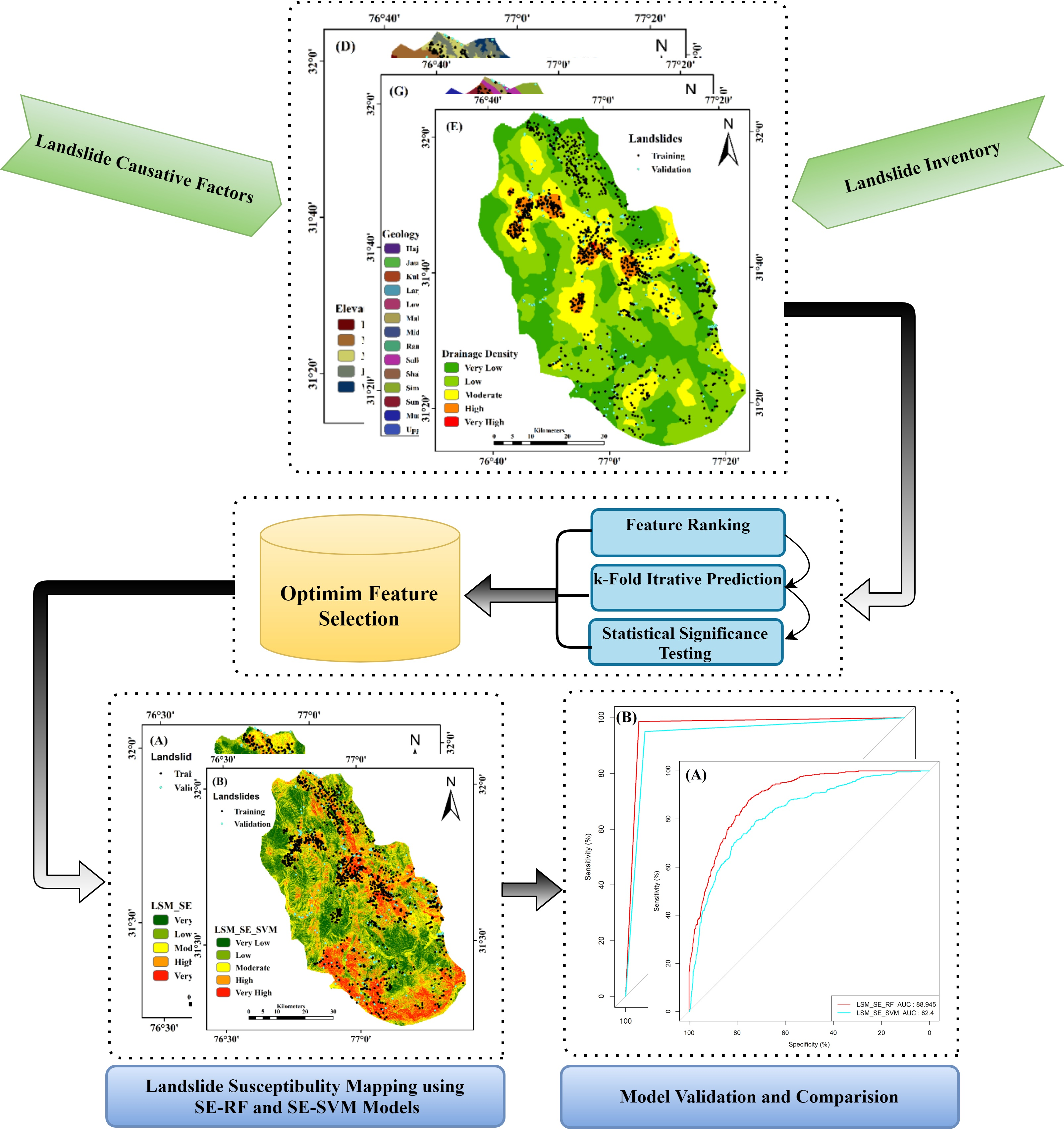
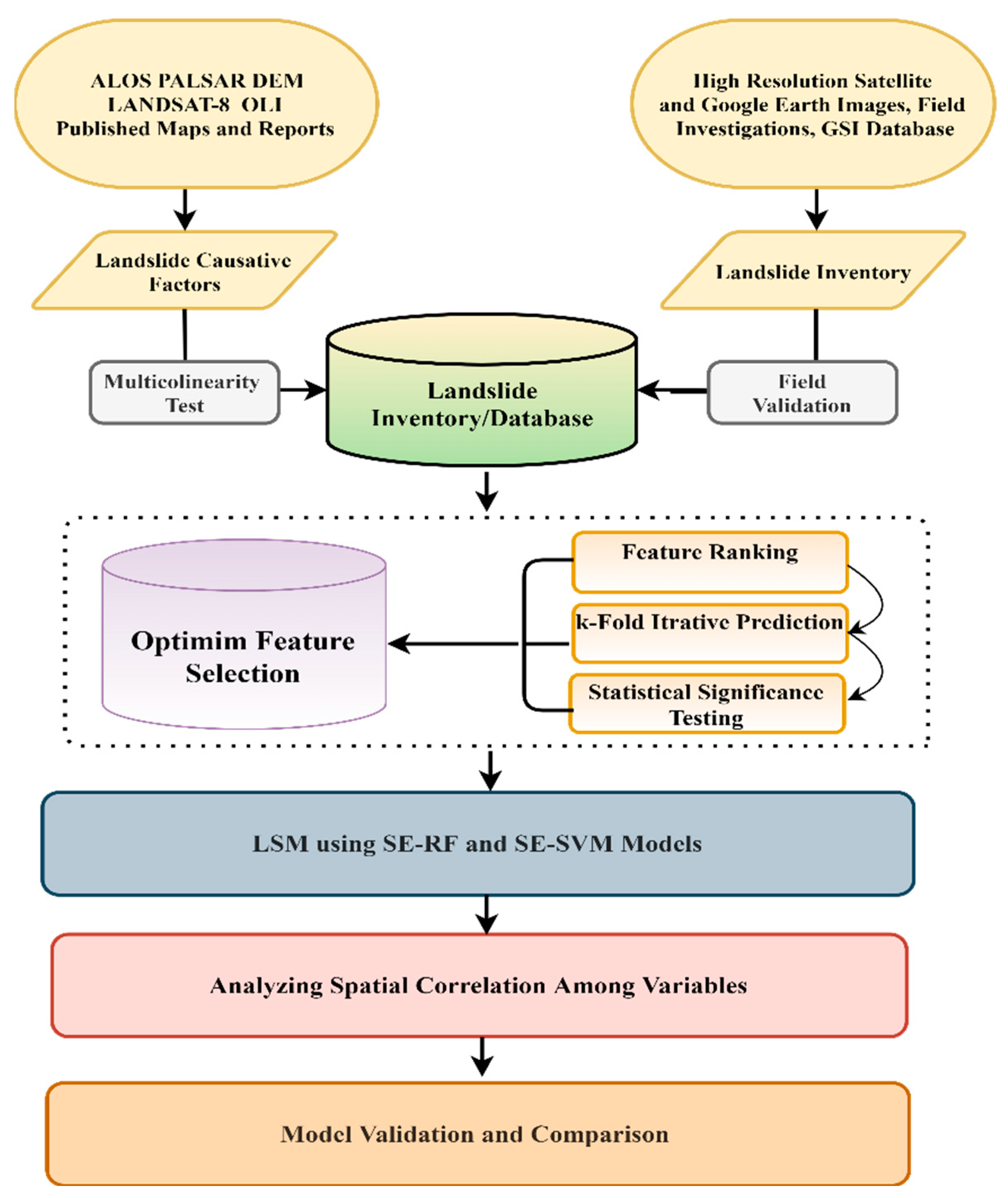
2. Materials and Methods

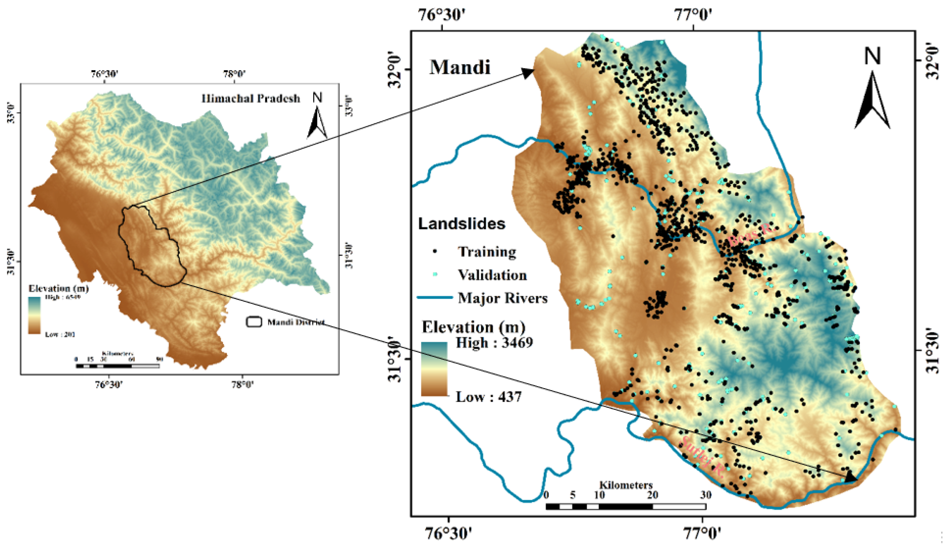
2.1. Study Area and Landslide Inventory

The Mandi district in the state of Himachal Pradesh, India, has geographic coordinates of 31°13’ and 32°05’ north latitudes and 76°37’ and 77°25’ east longitudes, and a 3951 km2 area (Figure 1). The area’s elevation increases from west to east and south to north, and ranges between 500 m to 3400 m. The area falls in the mid-hills-sub-humid zone and high hills temperate wet agro-climatic zone, which receives an annual average rainfall of 1240 mm and an annual temperature of 24 °C. The road density of the Mandi district is 155 km per 100 km2. The two major National Highways that run across the district’s length and breadth are NH-3 (Atari–Manali–Leh) and NH-154 (Pathankot–Sundernagar–Bilaspur). The Beas river runs through the northern part of the district whereas the southern part is drained by the Satluj river.
The landslide inventory map’s main elements include the geographical location of the landslide, its date and time of occurrence, triggering factors like heavy rainfall or earthquake, and damages incurred in terms of life and property [59]. The landslide inventory of the Mandi district was prepared by analyzing high-resolution satellite and Google Earth images, historical reports, and field surveys using handheld GPS (Figure 1). A total of 1723 rainfall-induced landslides and their location, type, and triggering factor, etc., were documented, with areas ranging from 26 m2 to 23,164 m2 and an average area of about 844 m2. Based on accepted terminology, the landslides were then categorized as shallow transitional slides with some deep rotational landslides [60]. Furthermore, it was found that a common triggering factor for all the landslides was rainfall during monsoon season and road construction activities in the region. The landslide inventory was further split into 1199 (70%) training and 524 (30%) validation datasets using a random sampling procedure in the ArcGIS environment.

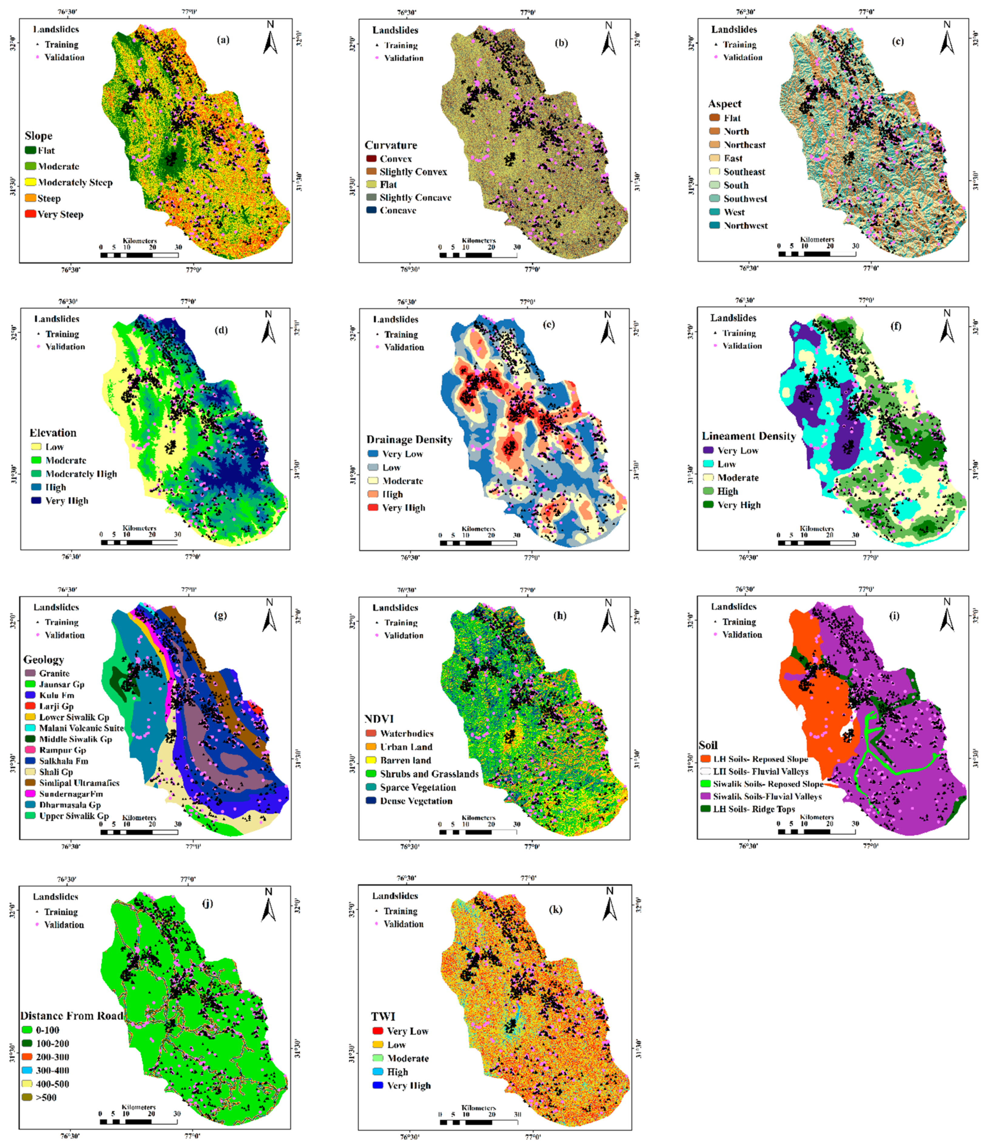
2.2. Landslide Causative Factors (LCF’s)

The interaction between geological, morphometric, topographical, and hydrological factors in a region influences landslides’ occurrence. Hence, the appropriate selection of these causative factors is a primary step in landslide susceptibility analysis [61]. In the present study, 14 landslide causative factors, namely, slope gradient, plan curvature, slope aspect, elevation, drainage density, lithology, geology, land use and landcover (LULC), normalized difference vegetation index (NDVI), soil characteristics, lineament density, stream power index (SPI), topographic wetness index (TWI), and distance from the roads, were identified using expert opinions and data availability. The list of various data sources is presented in Table 1. These factors were rasterized to a resolution of 30 m in the GIS environment.
An ALOS-PALSAR Digital Elevation Model (DEM) with a 12.5 m resolution was used to derive the elevation, slope gradient, slope aspect, curvature, topographical wetness index (TWI), stream power index, and drainage density of the study area using ArcGIS software. The slope gradient of an area is defined as the rate of change of elevation over a distance in the direction of the steepest fall that influences landslides in a particular area [62]. The slope gradient map was classified as flat (<15°), moderate (15–25°), moderately steep (25–35°), steep (35–45°), and very steep (>45°). The plan curvature of the slope represents the direction of the maximum slope and has an essential role in landslide occurrence as it controls the inflow and outflow of the drainage networks of an area [63]. The curvature map of the area was divided into five categories: convex, slight convex, flat, slightly concave, and concave. The slope’s aspect is the orientation of the slope, measured clockwise in degrees from 0 to 360, where 0 is north-facing, 90 is east-facing, 180 is south-facing, and 270 is west-facing. Aspect is again an essential parameter for better understanding the slope stability in a particular direction [64]. Elevation is extensively used in landslide susceptibility. Even though a direct relationship between landslide occurrences and elevation could not be established, it still affects other parameters like rainfall and seismicity [65]. The Beas river basin surrounds the northern part of the Mandi District. It is characterized by a lower elevation, including the Balh valley in the Mandi District. The southwestern part of the Mandi District is characterized by low to moderate elevation zones with elevations ranging from 600 to 1500 m. The drainage density of an area influences the surface runoff and slope erosion potential [52]. The Beas and Satluj rivers in the Mandi District, and their tributaries and distributaries, drain the area well. Although most of the study area has a very low drainage density, there is still a considerable area with a moderate to high drainage density and significant landslides. TWI is used to quantify the hydrological impact of the drainage networks on the wetness/saturation of the soils on the slopes. The greater the value of the TWI, greater is the soil’s water content, and the more significant is its hence tendency for erosion [66]. The TWI map was generated by the combined arithmetic applications of slope gradient and flow accumulation parameters, using TWI = (Ln (As)/Tan (β)), where Ln is the natural log, As is the flow accumulation, and β is the slope gradient in radians. The TWI of the area was classified into the following five categories: very low, low, moderate, high, and very high. Lineament density is defined as the total length of all of the lineaments divided by the area under study. Stream power index (SPI) describes the potential of flow erosion of a particular point on the topographic surface. In a given catchment area, the amount of water contributed by the upslope area increases with the increase in the slope gradient. This, in turn, increases the SPI and risk of erosion at a given point on the surface. An SPI map of the study area was also prepared by the combined arithmetic application of morphometric variables, which includes the slope gradient and flow accumulation parameters using SPI = As x Tan(β). The lineament density was computed using the line density tool in the GIS environment. The Operational Land Imager (OLI) and Thermal Infrared Sensor (TRIS) of the Landsat-8 satellite with 12-Band multispectral images with a 30-m resolution were procured from 2015 to 2020, from the first week of October to the last week of November, were considered adequate due to the availability of cloud-free data just after the monsoon season is over. The NDVI map is one of the most fundamental and widely accepted indexes to detect vegetation and landcover changes caused by infrastructural developmental activities [67]. NDVI provides information about landcover changes using the energy absorbed and emitted by the objects on the Earth’s surface, and is prepared by image analysis techniques on high-resolution Landsat-8 images using the following: NDVI = (NIR − RED)/(NIR + RED), where NIR (Near Infra-Red Band) and RED bands represent the spectral reflectance bands of the electromagnetic spectrum. The LULC characteristics of an area indicate the physical characteristics of the Earth’s surface and the change brought due to human interference. Deforestation, intensive agriculture, and new infrastructure development may lead to soil and slide degradation, which are the main causative factors for landslide occurrences [35]. The LULC map of the area was generated using Landsat-8 images by the maximum likelihood classification method in ERDAS Imagine software. An area’s geological and lithological boundaries are closely related to the slope and rock strength, and such boundaries may lead to increased landslide activity [61]. The study area lies within the lesser Himalayan region. The Jutog, Chail, Shah, and Tertiary group of rocks are predominant in the district. The oldest rocks belong to Jutog groups, whereas the youngest valley fills are of a recent age, comprising clay, sand, and gravel beds. The Jutog formation comprises slates, Schists, and Quartzite, with Hematite and magnetite bands included in Chail formation. The Granitic rocks are found to occur around the Karsog area. Thin bands of Slates are also found to occur. Salt grit, locally known as lokhan, is overlain by Mandi Darla volcanics [68]. The soil type is characterized by the percentage of sand, silt, and clay minerals present, configuring the soil’s texture and hydraulic properties. Even though it is not straightforward to define the complex relationship between the soil’s hydrological properties and the mechanics through which landslides occur, soils with a higher permeability still allow the water to flow through them, making them more susceptible to landslides. Additionally, different types of soils have different cohesion values. Therefore, the infiltrated water might erode the soils with lesser cohesion values [69]. Five soils were identified in the study area, along with their depth, drainage, and erosion properties. The road construction activities in mountainous regions result in loss of support and crack development due to an increased strain in the upper soil mass. In addition, road construction leads to a change in each area’s natural drainage corridor [70]. Hence, landslide occurrences are more common along the road alignment. The distance to the roads of the study area was divided into six classes: 0–100, 100–200, 200–300, 300–400, 400–500, and >500 m. The thematic layers of landslide causative factors were prepared using Arc GIS 10.4.1 and GEOMATICA. The mathematical calculations for statistical and machine learning methods were carried out in SPSS software and integrated R-ArcGIS bridge for spatial data analysis.
In the landslide susceptibility analysis, landslide causative factors are usually selected based on the area’s landslide categories, geological, and topographical characteristics [43]. As no definite guidelines are available for the optimum selection of these factors, many research studies selected these factors randomly or based on data availability. However, to avoid overfitting data and achieve the maximum predictive potential from the model, it is necessary to quantify and select the best-suited subset from the available factors and to remove non-essential factors with a low correlation to landslide occurrence [61]. Many researchers have used various techniques, like linear correlation, factor analysis, chi-square ranking, and multi-factor approach, to carry out feature selection process but encountered problems of excess time consumption and inability in order to decide the threshold for minimum factor inclusion in the model [71,72,73,74]. However, some studies have used a hybrid approach of combining feature ranking with a statistical significance test to select the optimum feature subset. The statistical significance indicates the level of confidence based on which a null hypothesis can be accepted or rejected. A hypothesis can only be accepted at a 95% significance level (p > 0.05) for the systematic pairwise difference between the different model performances. A k-fold cross-validation procedure is generally applied to split the dataset into subsets, allowing for different training samples for each process. In the present study, Chi-squared and information gain algorithms were used for feature ranking, logistic regression (LR) was used as the initial predictive model, and Wilcoxon’s Signed-Rank test and One-Sample T-Test were used to measure the statistical significance level to obtain the optimum feature subset. The detailed methodology of the study is depicted in Figure 2.

2.3. Shannon Entropy (SE) Model

The entropy of a system conceptually measures the degree of randomness, disorder, uncertainty, or instability of a system [6,33]. Claude Shannon, in 1948, developed the concept of entropy to analyze a fundamental communication problem of information theory, but later, this theory was found to be helpful in other areas. The concept of the entropy of landslides refers to the probability distribution of landslide occurrences concerning its frequency in each subclass of landslide causative factors [34,63]. Thus, entropy values can be used to calculate the relative weights of the data based on an index system using the following equations
E j = i = 1 N j P ij log 2 P ij ,   j = 1 , ,   n
E jmax =   log 2 N j ,   j = number   of   subclasses H j = ( E jmax E j E jmax ) ,   H = ( 0 , 1 ) ,   j = 1 , , n
W j = H j FR
where Ej and Ejmax are the entropy values, Hj is the information coefficient, and Nj is the number of classes in each landslide causative factor. Wj is the relative weight assigned to each landslide causative factor and FR is the frequency ratio value.

2.4. Random Forest (RF) Model

The RF model is a supervised learning algorithm that combines decision tree predictors. Each tree has randomly sampled independent data, and each tree fits independently in the data subset, achieved by splitting existing samples and regenerating random new samples using bootstrapping [75]. The RF model is a widely used model for regression and classification problems. It provides a high prediction accuracy, low errors, and can reduce the risk of overfitting [42,54]. To achieve good model performance and minimize the errors in the RF model, three hyperparameters are defined, namely: (i) the number of trees to be grown/combined (ntree), (iii) the maximum number of features to be considered at each split (mtree), and (iv) the size of the terminal nodes (nodesize).

2.5. Support Vector Machine (SVM) Model

SVM is a machine learning algorithm based on statistical learning and structural risk minimization theory [76]. The primary aim of SVM is to separate the non-linear dataset using an optimal hyperplane into two sample classes. The optimal classification hyperplane maximizes the margin of separation and splits the dataset points as ±1, where +1 refers to the presence and -1 refers to the absence of point on the classification hyperplane. The distance between the training points adjoining the classification hyperplane (support vectors) is known as the classification margin [77]. The activation kernel function transforms non-linear data into a higher dimensional feature space for linear classification. The kernel functions can be classified as linear, polynomial, radial, and sigmoid. Previous studies used these radial basis kernels, as well as polynomial kernel functions, the most in the landslide susceptibility analysis [78,79]. The optimum hyperplane is generated using the decision function f(x) = (ω.ϕ(x)) + b, where ω represents the coefficient vector defining the orientation of the classification hyperplane, ϕ(x) is the input sample x converted to high dimensional feature space, and b is the offset of hyperplane taken from origin.

3. Results

3.1. Multicollinearity Analysis

A multicollinearity test was conducted to identify the interdependence among the landslide causative factors. Any collinearity among variables can result in errors in output and decrease the model’s predictive potential [80]. Variance inflation factor (VIF) values > 10 or tolerance values < 0.1 suggest the problem of collinearity among the independent variables. Out of the 14 landslide causative factors initially selected for analysis, it was found that all factors have acceptable values of VIF and tolerance (Table 2). Hence, all 14 landslide causative factors were deemed suitable for further analysis of the optimum feature selection and landslide susceptibility analysis.

3.2. Optimum Selection of LCF’s

In the present study, landslide causative factors’ quality and usefulness were determined using information gain and Chi-square ranking algorithms. The logistic regression (LR) model was applied iteratively to access the prediction capabilities of feature datasets with an additional feature in each step.
A k-fold method was applied to split the landslide inventory dataset into 10 subsets to produce a new training dataset for each iterative step. It can be observed from Table 3 that both these methods produced different weights. In the next step, the Wilcoxon signed-rank test and One-Sample T-Test were applied as a statistical significance test for a pairwise comparison of the prediction models.
The results of all of the possible model scenarios are shown in Table 4. It was observed that Case-4 and Model-11 had relevant features, a high prediction performance, and a high confidence level, and were selected as the optimum feature subsets for further analyses. The selected features are shown in Figure 3.

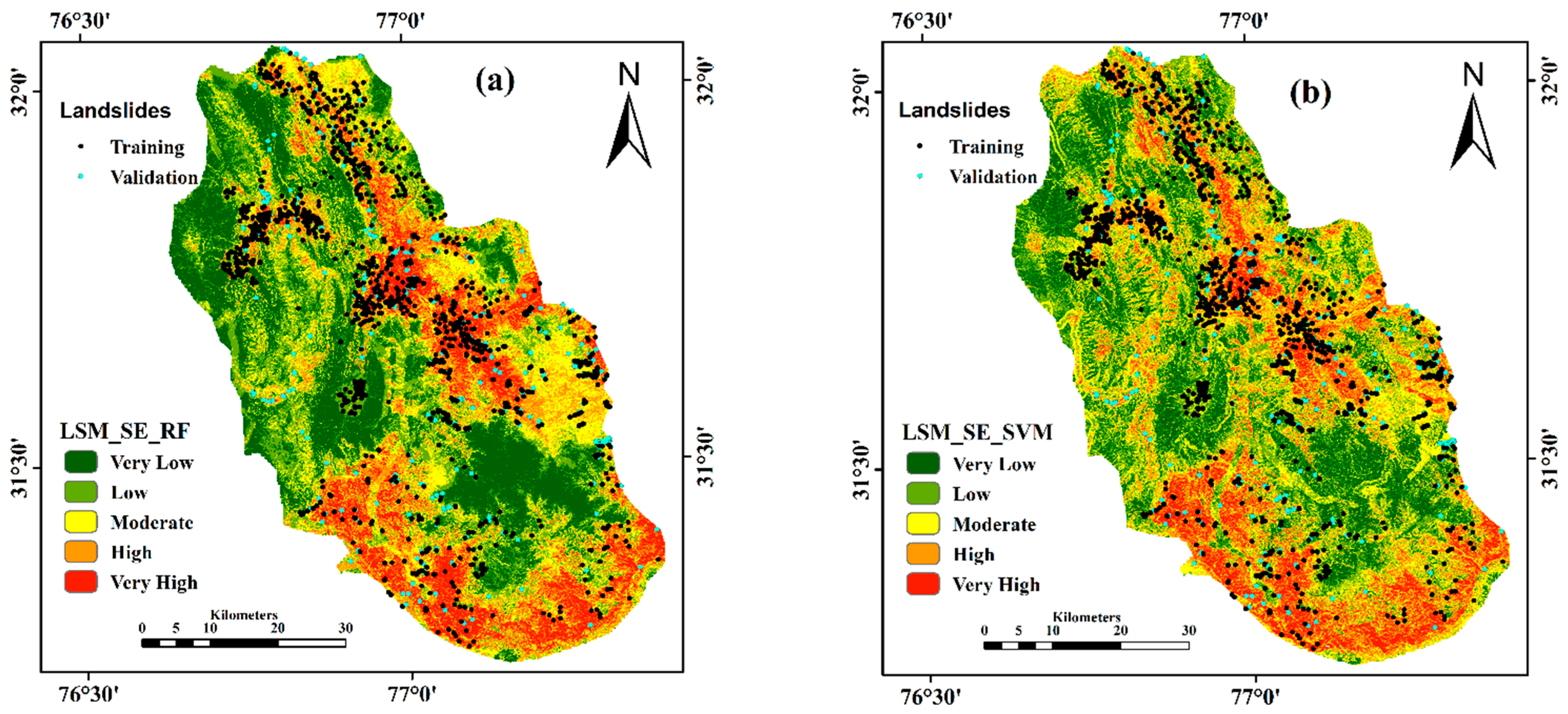
3.3. LSM Using SE-RF Model

The Ej values calculated for the Shannon entropy model were used to reclassify the subsets of landslide causative factors, and each factor was assigned a relative Wj value (Table 5). The landslide inventory data were split into 10-folds using the k-fold cross-validation method. These factors were then used as inputs for the FR model. The hyperparameters for the RF model were taken as ntree = 250, mtree = 5, and nodesize = 5. The LSM SE-RF produced was classified into five susceptibility classes, as follows: very low (0–0.196), low (0.196–0.372), moderate (0.372–0.552), high (0.552–0.745), and very high (0.745–1). The percentage of area in each susceptibility class was calculated as very low (22.47%), low (23.72%), moderate (22.12%), high (17.51%), and very high (14.17%; Figure 4a).

3.4. LSM Using SE-SVM Model

The 10 k-fold cross-validation dataset and landslide causative factors reclassified using SE model factors were considered as an input in the radial kernel-based SVM algorithm for calculating the LSMSE-SVM values. These values ranged from 0 to 1, where values closer to 0 indicated a lower probability of landslide occurrence and values closer to 1 indicated a higher probability of landslide occurrence. The LSM produced using the SE-SVM model was classified into five categories, namely very low (0–0.349), low (0.349–0.450), moderate (0.450–0.556), high (0.556–0.674), and very high (0.674–1) (Figure 4b), using the natural breaks classification method in a GIS environment. The LSMSE-SVM map analysis indicated that the study area percentage was very low, low, moderate, high, and very high, with 17.76%, 24.35%, 26.12%, 19.28%, and 12.49%, respectively (Figure 4b).
It was observed that the Wj values were the highest for the drainage density (0.269), TWI (0.140), and NDVI (0.121), and the ranking algorithms also suggested that these features had high ranking coefficients. Hence, these were identified as the primary factors responsible for higher landslide susceptibility in the study area.

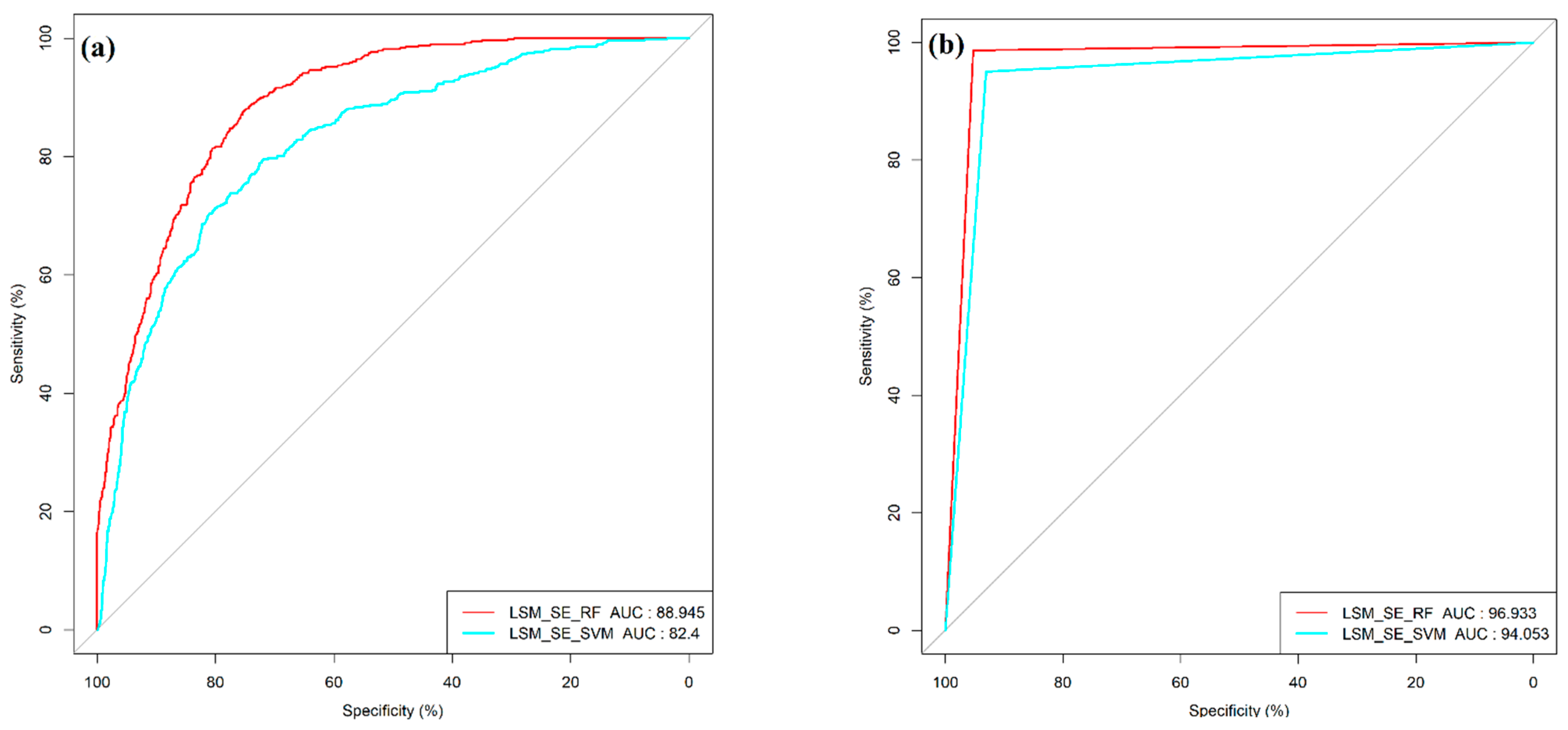
3.5. Performance and Validation of Models

In the present study, the predictive performance of the hybrid LSM models was evaluated using various statistical and visual performance metrics. The confusion matrix is generally used in classification problems. It represents the counts from actual and predicted values using true positive (TP), true negative (TN), false positive (FP), and false-negative (FN) values, where TP indicates the number of actual landslide pixels classified accurately, TN indicates the number of non-landslide pixels classified accurately, FP indicates the number of non-landslide pixels classified as landslides pixels, and FN indicates the number of actual landslide pixels classified as non-landslides pixels. The confusion matrix accuracy, precision, recall, root mean square error (RMSE), and mean absolute error (MAE) values were calculated. Receiver operating characteristic (ROC) curves with area under curve (AUC) values are generally used to access the classification performance. The higher the AUC’s value, the better the model is for accurately predicting the landslide and non-landslide pixels. The landslide inventory training dataset was used to generate the AUC prediction curve, while the validation dataset was used to generate the AUC validation curve and performance matrices. It was found that the SE-FR and SE-SVM models had training accuracies with AUC = 96.933 and AUC = 94.053, respectively. In contrast, the prediction capability of the models had AUC = 88.945 and AUC = 82.4 values, respectively (Figure 5). In terms of the results obtained from the confusion matrices, the SE-FR and SE-SVM models had values for accuracy of 0.896 and 0.854, precision of 0.958 and 0.931, respectively, and recall of 0.814 and 0.790, respectively. The MAE and RMSE values of the SE-FR and SE-SVM models were 0.135 and 0.174, and 0.295 and 0.347, respectively as shown in Table 6. The results of the prediction matrices indicate that both models have good accuracies, prediction, and recall values, and the MAE and RMSE errors generated in both models are under acceptable limits. Based on these statistical and visual performance metrics, it can be found that both models have a good predictive potential and acceptable values of errors.

4. Discussion

Statistical and ML modeling is an essential component for determining the landslide susceptibility of an area. The accuracy of statistical models depends on the data quality, appropriate landslide causative factors, and model structure. The process of the generation of landslide susceptibility maps is complex and requires a multistep analysis. The present study focusses on three main issues: (a) the optimum selection of landslide causative factors using feature selection process, (b) the mapping of landslide susceptibility of Mandi District using hybrid SE-RF and SE-SVM models, and (c) the comparison of these two hybrid models based on performance matrices. In the present study, 14 LCFs were evaluated to find the optimum subset. It was found that the feature selection process, which used a hybrid approach, resulted in the selection of 11 optimum feature subsets.
The analysis of the LSMs produced using SE-RF and SE-SVM models indicated that areas with high TWI values, particularly in the 0–100 m distance to roads, are highly prone to landslides. In mountainous regions like the study area, the continuous excavation of slopes for road construction activities and the infiltration of water, especially during monsoon season, results in an increased burden on slopes. The soil mass in such areas becomes unstable and often results in sliding. Lower elevation regions have seen such anthropological activities on a larger scale than the higher elevation regions of the study area. In addition, higher-elevation regions have less accessibility, and few landslides are reported.
Similarly, the analysis of the geology map confirms that the Middle Siwalik Group was highly prone to landslides due to the presence of sedimentary rocks like medium- to coarse-grained sandstone and conglomerate. The rest of the causative factors, such as curvature, aspect, and lineaments, have a lower influence on the landslide susceptibility of the region. Such a combination of LCF’s is seen in similar studies of mountainous regions [5,11,12,36,48,70,81].
RF and SVM are two highly efficient machine learning models that can tackle complex non-linear relationships among variables, and are readily used by researchers in classification problems. FR is a combined tree-based model that can handle high dimensional spaces and categorical features with a high accuracy and is easily interpretable. A disadvantage of the RF model is its incapacity to calculate the relative importance of each subclass of the landslide causative factors. SVM uses “support vectors” and performs better when data are sparce and non-linearly separable. SVM has the advantage of having non-linear kernel functions but has a higher tendency of overfitting. SE is a statistical bivariate model that can calculate the factors’ relative weights and subclasses with relative ease and minimal time consumption. The analysis of the results of this study indicated that the integration of SE-RF and SE-SVM models resulted in increased accuracy and efficiency for both models.
In comparison with each other, the SE-RF model performed better than the SE-SVM model. The SE-SVM model has a +2.88% higher AUC for model validation and +6.54% higher AUC for model prediction. The performance matrices also indicated an increase in +4.2% accuracy and +2.7% precision, with a 3.9% decrease in MAE and 5.2% decrease in RMSE errors. This may be attributed to the overdependence of the SVM model on data pre-processing and kernel functions. Such results are consistent with the findings of [80] who combined LR and SVM with the IOE method, who combined EBF method with RF to obtain landslide susceptibility, who used an ensemble of WOE with different kernel functions of SVM, and who used various DEM’s and an integrated FR-RF model for assessment of the landslide susceptibility. Thus, using a hybrid approach to integrate statistical and ML models helps eliminate the disadvantages of individual models and increases the overall efficiency prediction capabilities of the models.

5. Conclusions

The analysis of landslide susceptibility is the primary step in managing and mitigating landslide risk in a mountainous region. Many statistical and ML algorithms have been used in recent years, but no definitive method is considered best for preparing the LSM of a region. The hybrid integration of these methods has the advantage of a better prediction potential compared with individual models. In the present study, a statistical SE model is integrated with RF and SVM models to overcome the shortcomings of the individual method. A total of 14 LCFs (slope gradient, plan curvature, slope aspect, elevation, drainage density, lithology, geology, land use and landcover (LULC), normalized difference vegetation index (NDVI), soil characteristics, lineament density, stream power index (SPI), topographic wetness index (TWI), and distance from the roads) were identified. A feature selection process was carried out using two feature ranking algorithms, i.e., information gain and Chi-square, which were used to determine the individual scores of the LCFs, and Wilcoxon signed-rank test and One-Sample T-Test were used to determine the statistical significance of the factors. The results of both hybrid models indicated TWI and distance from roads to be the two primary factors responsible for landslide occurrences in the study area. The results also indicated that although both models performed satisfactorily, the SE-RF model had +2.88% and +6.54% higher AUC values than the SE-SVM model. The main advantage of such an approach is that only relevant LCFs were used to generate the LSM. The integration of models helps establish an effective spatial relationship between landslide occurrences and LCFs, while reducing overfitting problems. This study will help regional planners and stakeholders in effective landslide risk management and sustainable developmental activities.

Author Contributions

Conceptualization, A.S. and C.P.; methodology, A.S. and C.P.; software, A.S.; formal analysis, A.S.; investigation, A.S., C.P. and V.S.M.; resources, A.S.; data curation, A.S.; validation, A.S.; visualization, A.S., C.P. and V.S.M.; writing—original draft preparation, A.S.; writing—review and editing, A.S., C.P. and V.S.M.; supervision, C.P. and V.S.M. All authors have read and agreed to the published version of the manuscript.

Funding

This research received no external funding.

Conflicts of Interest

The authors declared no conflict of interest.

References

  1. Ali, S.A.; Parvin, F.; Vojteková, J.; Costache, R.; Linh, N.T.T.; Pham, Q.B.; Vojtek, M.; Gigović, L.; Ahmad, A.; Ghorbani, M.A. GIS-based landslide susceptibility modeling: A comparison between fuzzy multi-criteria and machine learning algorithms. Geosci. Front. 2020, 12, 857–876. [Google Scholar] [CrossRef]
  2. Wang, G.; Lei, X.; Chen, W.; Shahabi, H.; Shirzadi, A. Hybrid Computational Intelligence Methods for Landslide Susceptibility Mapping. Symmetry 2020, 12, 325. [Google Scholar] [CrossRef] [Green Version]
  3. Landslides. Available online: https://www.who.int/health-topics/landslides#tab=tab_1 (accessed on 15 September 2021).
  4. Revenue Department, Government of Himachal Pradesh. Memorandum of Damages Due to Flash Floods, Cloudbursts and Landslides during Monsoon Season-2020; HPSDMA: Shimla, India, 2020; pp. 14–26.
  5. Zhao, X.; Chen, W. Optimization of Computational Intelligence Models for Landslide Susceptibility Evaluation. Remote Sens. 2020, 12, 2180. [Google Scholar] [CrossRef]
  6. Nohani, E.; Moharrami, M.; Sharafi, S.; Khosravi, K.; Pradhan, B.; Pham, B.T.; Lee, S.; Melesse, A.M. Landslide Susceptibility Mapping Using Different GIS-Based Bivariate Models. Water 2019, 11, 1402. [Google Scholar] [CrossRef] [Green Version]
  7. Nayak, J.; Westen, C.V.; Das, I.C.; Nayak, J. Landslide Risk Assessment along a Major Road Corridor Based on Historical Landslide Inventory and Traffic Analysis; University of Twente Faculty of Geo-Information and Earth Observation (ITC): Enschede, The Netherlands, 2010; p. 104. [Google Scholar]
  8. Reichenbach, P.; Rossi, M.; Malamud, B.; Mihir, M.; Guzzetti, F. A review of statistically-based landslide susceptibility models. Earth-Sci. Rev. 2018, 180, 60–91. [Google Scholar] [CrossRef]
  9. Feizizadeh, B.; Jankowski, P.; Blaschke, T. A GIS based spatially-explicit sensitivity and uncertainty analysis approach for multi-criteria decision analysis. Comput. Geosci. 2013, 64, 81–95. [Google Scholar] [CrossRef] [Green Version]
  10. Saha, A.; Saha, S. Comparing the efficiency of weight of evidence, support vector machine and their ensemble approaches in landslide susceptibility modelling: A study on Kurseong region of Darjeeling Himalaya, India. Remote Sens. Appl. Soc. Environ. 2020, 19, 100323. [Google Scholar] [CrossRef]
  11. Arabameri, A.; Karimi-Sangchini, E.; Pal, S.; Saha, A.; Chowdhuri, I.; Lee, S.; Bui, D.T. Novel Credal Decision Tree-Based Ensemble Approaches for Predicting the Landslide Susceptibility. Remote Sens. 2020, 12, 3389. [Google Scholar] [CrossRef]
  12. Chen, W.; Pourghasemi, H.R.; Panahi, M.; Kornejady, A.; Wang, J.; Xie, X.; Cao, S. Spatial prediction of landslide susceptibility using an adaptive neuro-fuzzy inference system combined with frequency ratio, generalized additive model, and support vector machine techniques. Geomorphology 2017, 297, 69–85. [Google Scholar] [CrossRef]
  13. Shahabi, H.; Khezri, S.; Bin Ahmad, B.; Hashim, M. RETRACTED: Landslide susceptibility mapping at central Zab basin, Iran: A comparison between analytical hierarchy process, frequency ratio and logistic regression models. CATENA 2014, 115, 55–70. [Google Scholar] [CrossRef]
  14. Galli, M.; Ardizzone, F.; Cardinali, M.; Guzzetti, F.; Reichenbach, P. Comparing landslide inventory maps. Geomorphology 2008, 94, 268–289. [Google Scholar] [CrossRef]
  15. Ngadisih; Bhandary, N.P.; Yatabe, R.; Dahal, R.K. Logistic regression and artificial neural network models for mapping of regional-scale landslide susceptibility in volcanic mountains of West Java (Indonesia). AIP 2016, 1730, 60001. [Google Scholar] [CrossRef]
  16. Sharma, R.K.; Mehta, B.S. Macro-zonation of landslide susceptibility in Garamaura-Swarghat-Gambhar section of national highway 21, Bilaspur District, Himachal Pradesh (India). Nat. Hazards 2011, 60, 671–688. [Google Scholar] [CrossRef]
  17. Banshtu, R.S.; Prakash, C. Application of Remote Sensing and GIS Techniques in Landslide Hazard Zonation of Hilly Terrain; Springer: Cham, Switzerland, 2014; pp. 313–317. [Google Scholar] [CrossRef]
  18. Lee, S.; Lee, M.-J.; Jung, H.-S.; Lee, S. Landslide Susceptibility Mapping Using Naïve Bayes and Bayesian Network Models in Umyeonsan, Korea. Geocarto Int. 2019, 35, 1665–1679. [Google Scholar] [CrossRef]
  19. Bui, D.T.; Shahabi, H.; Shirzadi, A.; Chapi, K.; Alizadeh, M.; Chen, W.; Mohammadi, A.; Bin Ahmad, B.; Panahi, M.; Hong, H.; et al. Landslide Detection and Susceptibility Mapping by AIRSAR Data Using Support Vector Machine and Index of Entropy Models in Cameron Highlands, Malaysia. Remote Sens. 2018, 10, 1527. [Google Scholar] [CrossRef] [Green Version]
  20. Alvioli, M.; Mondini, A.; Fiorucci, F.; Cardinali, M.; Marchesini, I. Automatic Landslide Mapping from Satellite Imagery with a Topography-Driven Thresholding Algorithm. PeerJ Prepr. 2018, 1–4. [Google Scholar] [CrossRef] [Green Version]
  21. Nagarajan, R.; Mukherjee, A.; Roy, A.; Khire, M.V. Technical note Temporal remote sensing data and GIS application in landslide hazard zonation of part of Western ghat, India. Int. J. Remote Sens. 1998, 19, 573–585. [Google Scholar] [CrossRef]
  22. Bui, D.T.; Pradhan, B.; Lofman, O.; Revhaug, I.; Dick, O.B. Spatial prediction of landslide hazards in Hoa Binh province (Vietnam): A comparative assessment of the efficacy of evidential belief functions and fuzzy logic models. CATENA 2012, 96, 28–40. [Google Scholar] [CrossRef]
  23. Shahri, A.A.; Spross, J.; Johansson, F.; Larsson, S. Landslide susceptibility hazard map in southwest Sweden using artificial neural network. CATENA 2019, 183, 104225. [Google Scholar] [CrossRef]
  24. Frangov, G.; Petkova, V.; Stoyanov, V.; Kadiyski, M.; Kostov, V.; Papaliangas, T. Landslide Risk Assessment and Mitigation Along a Road in Sw Bulgaria. Fresenius Environ. Bull. 2017, 26, 244–253. [Google Scholar]
  25. Pradhan, B.; Abokharima, M.H.; Jebur, M.N.; Tehrany, M.S. Land subsidence susceptibility mapping at Kinta Valley (Malaysia) using the evidential belief function model in GIS. Nat. Hazards 2014, 73, 1019–1042. [Google Scholar] [CrossRef]
  26. Mandal, S.; Mondal, S. Statistical Approaches for Landslide Susceptibility Assessment and Prediction; Springer International Publishing: Cham, Switzerland, 2019; Available online: https://0-doi-org.brum.beds.ac.uk/10.1007/978-3-319-93897-4 (accessed on 25 September 2020).
  27. Ozdemir, A.; Altural, T. A comparative study of frequency ratio, weights of evidence and logistic regression methods for landslide susceptibility mapping: Sultan Mountains, SW Turkey. J. Asian Earth Sci. 2013, 64, 180–197. [Google Scholar] [CrossRef]
  28. Zare, M.; Jouri, M.H.; Salarian, T.; Askarizadeh, D. Comparing of Bivariate Statistic, AHP and Combination Methods to Predict the Landslide Hazard in Northern Aspect of Alborz Mt (Iran). Int. J. Agric. Crop Sci. 2014, 7, 543–554. [Google Scholar]
  29. Chen, W.; Xie, X.; Peng, J.; Shahabi, H.; Hong, H.; Bui, D.T.; Duan, Z.; Li, S.; Zhu, A.-X. GIS-based landslide susceptibility evaluation using a novel hybrid integration approach of bivariate statistical based random forest method. CATENA 2018, 164, 135–149. [Google Scholar] [CrossRef]
  30. Devkota, K.C.; Regmi, A.D.; Pourghasemi, H.R.; Yoshida, K.; Pradhan, B.; Ryu, I.C.; Dhital, M.R.; Althuwaynee, O.F. Landslide susceptibility mapping using certainty factor, index of entropy and logistic regression models in GIS and their comparison at Mugling–Narayanghat road section in Nepal Himalaya. Nat. Hazards 2012, 65, 135–165. [Google Scholar] [CrossRef]
  31. Liu, W.; Song, Z. Review of studies on the resilience of urban critical infrastructure networks. Reliab. Eng. Syst. Saf. 2019, 193, 106617. [Google Scholar] [CrossRef]
  32. Pourghasemi, H.R.; Pradhan, B.; Gokceoglu, C. Remote Sensing Data Derived Parameters and its Use in Landslide Susceptibility Assessment Using Shannon’s Entropy and GIS. Appl. Mech. Mater. 2012, 225, 486–491. [Google Scholar] [CrossRef]
  33. Milaghardan, A.H.; Abbaspour, R.A.; Khalesian, M. Evaluation of the effects of uncertainty on the predictions of landslide occurrences using the Shannon entropy theory and Dempster–Shafer theory. Nat. Hazards 2019, 100, 49–67. [Google Scholar] [CrossRef]
  34. Roodposhti, M.S.; Aryal, J.; Shahabi, H.; Safarrad, T. Fuzzy Shannon Entropy: A Hybrid GIS-Based Landslide Susceptibility Mapping Method. Entropy 2016, 18, 343. [Google Scholar] [CrossRef]
  35. Roy, J.; Saha, S.; Arabameri, A.; Blaschke, T.; Bui, D.T. A Novel Ensemble Approach for Landslide Susceptibility Mapping (LSM) in Darjeeling and Kalimpong Districts, West Bengal, India. Remote Sens. 2019, 11, 2866. [Google Scholar] [CrossRef] [Green Version]
  36. Yusof, N.M.; Pradhan, B.; Shafri, H.Z.M.; Jebur, M.N.; Yusoff, Z.M. Spatial landslide hazard assessment along the Jelapang Corridor of the North-South Expressway in Malaysia using high resolution airborne LiDAR data. Arab. J. Geosci. 2015, 8, 9789–9800. [Google Scholar] [CrossRef]
  37. Pradhan, A.M.S.; Kim, Y.-T. Spatial data analysis and application of evidential belief functions to shallow landslide susceptibility mapping at Mt. Umyeon, Seoul, Korea. Bull. Int. Assoc. Eng. Geol. 2016, 76, 1263–1279. [Google Scholar] [CrossRef]
  38. Budimir, M.E.A.; Atkinson, P.M.; Lewis, H.G. A systematic review of landslide probability mapping using logistic regression. Landslides 2015, 12, 419–436. [Google Scholar] [CrossRef] [Green Version]
  39. Yousefi, S.; Pourghasemi, H.R.; Emami, S.N.; Pouyan, S.; Eskandari, S.; Tiefenbacher, J.P. A machine learning framework for multi-hazards modeling and mapping in a mountainous area. Sci. Rep. 2020, 10, 1–14. [Google Scholar] [CrossRef]
  40. Saha, S.; Paul, G.C.; Pradhan, B.; Maulud, K.N.A.; Alamri, A.M. Integrating multilayer perceptron neural nets with hybrid ensemble classifiers for deforestation probability assessment in Eastern India. Geomat. Nat. Hazards Risk 2020, 12, 29–62. [Google Scholar] [CrossRef]
  41. Chang, K.-T.; Merghadi, A.; Yunus, A.P.; Pham, B.T.; Dou, J. Evaluating scale effects of topographic variables in landslide susceptibility models using GIS-based machine learning techniques. Sci. Rep. 2019, 9, 1–21. [Google Scholar] [CrossRef] [Green Version]
  42. Sahin, E.K.; Colkesen, I.; Acmali, S.S.; Akgun, A.; Aydinoglu, A.C. Developing comprehensive geocomputation tools for landslide susceptibility mapping: LSM tool pack. Comput. Geosci. 2020, 144, 104592. [Google Scholar] [CrossRef]
  43. Dou, J.; Bui, D.T.; Yunus, A.P.; Jia, K.; Song, X.; Revhaug, I.; Xia, H.; Zhu, Z. Optimization of Causative Factors for Landslide Susceptibility Evaluation Using Remote Sensing and GIS Data in Parts of Niigata, Japan. PLoS ONE 2015, 10, e0133262. [Google Scholar] [CrossRef] [Green Version]
  44. Hong, H.; Liu, J.; Zhu, A.-X. Modeling landslide susceptibility using LogitBoost alternating decision trees and forest by penalizing attributes with the bagging ensemble. Sci. Total Environ. 2020, 718, 137231. [Google Scholar] [CrossRef]
  45. Pham, B.T.; Bui, D.T.; Prakash, I.; Dholakia, M.B. Rotation forest fuzzy rule-based classifier ensemble for spatial prediction of landslides using GIS. Nat. Hazards 2016, 83, 97–127. [Google Scholar] [CrossRef]
  46. Duch, W.; Wieczorek, T.; Biesiada, J.; Blachnik, M. Comparison of feature ranking methods based on information entropy. In Proceedings of the 2004 IEEE International Joint Conference on Neural Networks, Budapest, Hungary, 25–29 July 2004; Volume 2, pp. 1415–1419. [Google Scholar] [CrossRef]
  47. Nguyen, V.V.; Pham, B.T.; Vu, B.T.; Prakash, I.; Jha, S.; Shahabi, H.; Shirzadi, A.; Ba, D.N.; Kumar, R.; Chatterjee, J.M.; et al. Hybrid Machine Learning Approaches for Landslide Susceptibility Modeling. Forests 2019, 10, 157. [Google Scholar] [CrossRef] [Green Version]
  48. Pradhan, B.; Lee, S. Landslide susceptibility assessment and factor effect analysis: Backpropagation artificial neural networks and their comparison with frequency ratio and bivariate logistic regression modelling. Environ. Model. Softw. 2010, 25, 747–759. [Google Scholar] [CrossRef]
  49. Youssef, A.M.; Pourghasemi, H.R. Landslide susceptibility mapping using machine learning algorithms and comparison of their performance at Abha Basin, Asir Region, Saudi Arabia. Geosci. Front. 2020, 12, 639–655. [Google Scholar] [CrossRef]
  50. Polykretis, C.; Chalkias, C. Comparison and evaluation of landslide susceptibility maps obtained from weight of evidence, logistic regression, and artificial neural network models. Nat. Hazards 2018, 93, 249–274. [Google Scholar] [CrossRef]
  51. Dou, J.; Yunus, A.P.; Bui, D.T.; Merghadi, A.; Sahana, M.; Zhu, Z.; Chen, C.-W.; Khosravi, K.; Yang, Y.; Pham, B.T. Assessment of advanced random forest and decision tree algorithms for modeling rainfall-induced landslide susceptibility in the Izu-Oshima Volcanic Island, Japan. Sci. Total Environ. 2019, 662, 332–346. [Google Scholar] [CrossRef] [PubMed]
  52. Chen, W.; Xie, X.; Peng, J.; Wang, J.; Duan, Z.; Hong, H. GIS-based landslide susceptibility modelling: A comparative assessment of kernel logistic regression, Naïve-Bayes tree, and alternating decision tree models. Geomat. Nat. Hazards Risk 2017, 8, 950–973. [Google Scholar] [CrossRef] [Green Version]
  53. Huang, Y.; Zhao, L. Review on landslide susceptibility mapping using support vector machines. CATENA 2018, 165, 520–529. [Google Scholar] [CrossRef]
  54. Merghadi, A.; Yunus, A.P.; Dou, J.; Whiteley, J.; ThaiPham, B.; Bui, D.T.; Avtar, R.; Abderrahmane, B. Machine learning methods for landslide susceptibility studies: A comparative overview of algorithm performance. Earth-Sci. Rev. 2020, 207, 103225. [Google Scholar] [CrossRef]
  55. Chen, W.; Zhang, S.; Li, R.; Shahabi, H. Performance evaluation of the GIS-based data mining techniques of best-first decision tree, random forest, and naïve Bayes tree for landslide susceptibility modeling. Sci. Total Environ. 2018, 644, 1006–1018. [Google Scholar] [CrossRef] [PubMed]
  56. Li, Y.; Chen, W. Landslide Susceptibility Evaluation Using Hybrid Integration of Evidential Belief Function and Machine Learning Techniques. Water 2019, 12, 113. [Google Scholar] [CrossRef] [Green Version]
  57. Chen, X.; Chen, W. GIS-based landslide susceptibility assessment using optimized hybrid machine learning methods. CATENA 2020, 196, 104833. [Google Scholar] [CrossRef]
  58. Survey, C.G.; Paper, C.; John, C.; California, W.; Survey, G.; Ca, S.; Calif, B.S.; Survey, G. Landslide Inventory Maps of Highway Corridors in California. In Proceedings of the 3rd North American Symposium on Landslides, Roanoke, VA, USA, 4–8 June 2017; pp. 529–540. [Google Scholar]
  59. Varnes, D.J. Landslide Hazard Zonation A Review of Principles and Practice, Natural Hazards; UNESCO: Paris, France, 1984; Available online: https://www.scirp.org/(S(351jmbntvnsjt1aadkposzje))/reference/ReferencesPapers.aspx?ReferenceID=1768332 (accessed on 6 August 2021).
  60. Fell, R. Landslide risk assessment and acceptable risk. Can. Geotech. J. 1994, 31, 261–272. [Google Scholar] [CrossRef]
  61. Arca, D.; Citiroglu, H.K.; Tasoglu, I.K. A comparison of GIS-based landslide susceptibility assessment of the Satuk village (Yenice, NW Turkey) by frequency ratio and multi-criteria decision methods. Environ. Earth Sci. 2019, 78, 81. [Google Scholar] [CrossRef]
  62. Jiménez-Perálvarez, J.D.; Irigaray, C.; El Hamdouni, R.; Chacón, J. Landslide-susceptibility mapping in a semi-arid mountain environment: An example from the southern slopes of Sierra Nevada (Granada, Spain). Bull. Int. Assoc. Eng. Geol. 2010, 70, 265–277. [Google Scholar] [CrossRef]
  63. Chen, W.; Fan, L.; Li, C.; Pham, B.T. Spatial Prediction of Landslides Using Hybrid Integration of Artificial Intelligence Algorithms with Frequency Ratio and Index of Entropy in Nanzheng County, China. Appl. Sci. 2019, 10, 29. [Google Scholar] [CrossRef] [Green Version]
  64. Pradhan, B. Remote sensing and GIS-based landslide hazard analysis and cross-validation using multivariate logistic regression model on three test areas in Malaysia. Adv. Space Res. 2010, 45, 1244–1256. [Google Scholar] [CrossRef]
  65. Choubey, V.M.; Mukherjee, P.K.; Bajwa, B.J.S.; Walia, V. Geological and tectonic influence on water–soil–radon relationship in Mandi–Manali area, Himachal Himalaya. Environ. Earth Sci. 2006, 52, 1163–1171. [Google Scholar] [CrossRef]
  66. Baum, R.L.; Godt, J. Early warning of rainfall-induced shallow landslides and debris flows in the USA. Landslides 2009, 7, 259–272. [Google Scholar] [CrossRef]
  67. Chen, W.; Li, Y. GIS-based evaluation of landslide susceptibility using hybrid computational intelligence models. CATENA 2020, 195, 104777. [Google Scholar] [CrossRef]
  68. Lee, S.; Talib, J.A. Probabilistic landslide susceptibility and factor effect analysis. Environ. Earth Sci. 2005, 47, 982–990. [Google Scholar] [CrossRef]
  69. Tsangaratos, P.; Ilia, I. Comparison of a logistic regression and Naïve Bayes classifier in landslide susceptibility assessments: The influence of models complexity and training dataset size. CATENA 2016, 145, 164–179. [Google Scholar] [CrossRef]
  70. Liu, L.-L.; Yang, C.; Wang, X.-M. Landslide Susceptibility Assessment Using Feature Selection-Based Machine Learning Models. Geomech. Eng. 2020, 25, 1–16. [Google Scholar]
  71. Laborda, J.; Ryoo, S. Feature Selection in a Credit Scoring Model. Mathematics 2021, 9, 746. [Google Scholar] [CrossRef]
  72. Breiman, L. Random Forests. Mach. Learn. 2001, 45, 5–32. [Google Scholar] [CrossRef] [Green Version]
  73. Cortes, C.; Vapnik, V. Support-vector networks. Mach. Learn. 1995, 20, 273–297. [Google Scholar] [CrossRef]
  74. Micheletti, N.; Foresti, L.; Robert, S.; Leuenberger, M.; Pedrazzini, A.; Jaboyedoff, M.; Kanevski, M. Machine Learning Feature Selection Methods for Landslide Susceptibility Mapping. Math. Geol. 2013, 46, 33–57. [Google Scholar] [CrossRef] [Green Version]
  75. Dou, J.; Yunus, A.P.; Bui, D.T.; Merghadi, A.; Sahana, M.; Zhu, Z.; Chen, C.-W.; Han, Z.; Pham, B.T. Improved landslide assessment using support vector machine with bagging, boosting, and stacking ensemble machine learning framework in a mountainous watershed, Japan. Landslides 2019, 17, 641–658. [Google Scholar] [CrossRef]
  76. Cigdem, O.; Demirel, H. Performance analysis of different classification algorithms using different feature selection methods on Parkinson’s disease detection. J. Neurosci. Methods 2018, 309, 81–90. [Google Scholar] [CrossRef]
  77. Zhang, T.; Han, L.; Chen, W.; Shahabi, H. Hybrid Integration Approach of Entropy with Logistic Regression and Support Vector Machine for Landslide Susceptibility Modeling. Entropy 2018, 20, 884. [Google Scholar] [CrossRef] [Green Version]
  78. Dou, J.; Yunus, A.P.; Bui, D.T.; Sahana, M.; Chen, C.-W.; Zhu, Z.; Wang, W.; Pham, B.T. Evaluating GIS-Based Multiple Statistical Models and Data Mining for Earthquake and Rainfall-Induced Landslide Susceptibility Using the LiDAR DEM. Remote Sens. 2019, 11, 638. [Google Scholar] [CrossRef] [Green Version]
  79. Pourghasemi, H.R.; Kerle, N. Random forests and evidential belief function-based landslide susceptibility assessment in Western Mazandaran Province, Iran. Environ. Earth Sci. 2016, 75, 1–17. [Google Scholar] [CrossRef]
  80. Arabameri, A.; Saha, S.; Roy, J.; Chen, W.; Blaschke, T.; Bui, D.T. Landslide Susceptibility Evaluation and Management Using Different Machine Learning Methods in The Gallicash River Watershed, Iran. Remote Sens. 2020, 12, 475. [Google Scholar] [CrossRef] [Green Version]
  81. Arabameri, A.; Pradhan, B.; Rezaei, K.; Lee, C.-W. Assessment of Landslide Susceptibility Using Statistical- and Artificial Intelligence-based FR–RF Integrated Model and Multiresolution DEMs. Remote Sens. 2019, 11, 999. [Google Scholar] [CrossRef] [Green Version]
Figure 1. Study area: Mandi District, Himachal Pradesh, with landslide training and validation datasets.
Geomatics 01 00023 g001
Figure 2. Flowchart depicting the methodology used in the study.
Geomatics 01 00023 g002
Figure 3. Landslide causative factors: (a) slope gradient, (b) curvature, (c) slope aspect, (d) elevation, (e) drainage density, (f) lineament density, (g) geology, (h) NDVI, (i) soil, (j) distance from roads, and (k) TWI.
Geomatics 01 00023 g003
Figure 4. Landslide susceptibility maps: (a) SE-RF model and (b) SE-SVM model.
Geomatics 01 00023 g004
Figure 5. ROC curves with AUC values: (a) AUC prediction and (b) AUC validation.
Geomatics 01 00023 g005
Table 1. Data purpose and sources for landslide susceptibility mapping.
DataData PurposeData SourceScale/Resolution
District Administration Mandi, Himachal PradeshAdministrative boundary of Mandihttps://hpmandi.nic.in/map-of-district/
(accessed on 20 September 2020)
1:50,000
H.P. Disaster Revenue Reports (2015–2019), Google Earth, GSI-BHUKOSH, Handheld GPSLandslide inventoryhttps://hpsdma.nic.in/
https://bhukosh.gsi.gov.in/
(accessed on 25 September 2020
1:50,000
ALOS-PALSAR DEMSlope, curvature, aspect, elevation, drainage density, and TWIhttps://search.asf.alaska.edu
(accessed on 12 October 2020)
12.5 m
Landsat-8 OLINDVI and lineamentshttp://earthexplored.usgs.gov
(accessed on 7 October 2020)
30 m
Geological Survey of India (GSI), BHUKOSHGeology and lithologyhttps://bhukosh.gsi.gov.in/
(accessed on 17 July 2020)
1:50,000
Ministry of Road Transport and Highways (MoRTH)Major roads of Mandi districthttps://morth.nic.in/
(accessed on 22 July 2020)
1:50,000
National Bureau of Soil Survey and Land Use Planning (ICAR-NBSS and LUP)Soil-Type, depth, and drainage of Mandi Districthttps://www.nbsslup.in/
(accessed on 19 July 2020)
1:50,000
Table 2. Multicollinearity coefficients for landslide causative factors.
ModelCollinearity Statistics
ToleranceVIF
Slope0.7983.658
Aspect0.5572.784
Curvature0.2175.633
Elevation0.4512.741
Drainage Density0.7515.214
Lineament Density3667.212
Geology0.4211.322
NDVI0.2576.369
Soil0.7854.321
Roads0.7412.357
TWI0.6794.212
Table 3. Feature weights and order using feature ranking algorithms.
Information GainChi-Squared
TWI0.301Distance to Roads0.579
Drainage Density0.247TWI0.447
Distance to Roads0.158Slope Gradient0.438
NDVI0.147Drainage Density0.301
Plan Curvature0.121Soil0.295
Slope Gradient0.123Geology0.278
Geology0.097Elevation0.199
Elevation0.082Slope Aspect0.154
Slope Aspect0.065NDVI0.125
Soil0.047Plan Curvature0.081
Lineament Density0.031Lineament Density0.065
SPI0.020LULC0.042
Lithology0.012Lithology0.015
LULC0.010SPI0.008
Table 4. Optimum feature subset using the feature selection process.
Feature Ranking MethodsCase No.Statistical TestsModel and Subset SizeFeatures in the Optimum Subset
Information GainCase-1One Sample T-TestModel-12Slope; Aspect; Curvature; Elevation; Drainage Density; Lithology; NDVI; LULC; Soil; SPI; TWI Distance to Roads
Case-2Wilcoxon Signed-Rank TestModel-11Slope; Aspect; Curvature; Elevation; Drainage Density; Geology; NDVI; Lineament Density; SPI; TWI; Distance from Roads
Chi-SquaredCase-3One Sample T-TestModel-9Slope; Curvature; Drainage Density; Geology; LULC; Soil; Lineament Density; SPI; Distance to Roads
Case-4Wilcoxon Signed-Rank TestModel-11Slope; Aspect; Curvature; Elevation; Drainage Density; Geology; NDVI; Soil; Lineament Density; TWI; Distance from Roads
Table 5. Spatial correlation between landslide occurrence and landslide causative factors.
Class PixelsPercent of PixelsLandslide PixelsPercent of PixelsFrequency RatioShanon Entropy
FR ValuesPijWj
Landslide Causative Factors
Slope Gradient (Degree)
Flat (<15°)435,0140.10290.0080.0790.0160.093
Moderate (15–25°)948,2590.222850.0760.3410.069
Moderately Steep (25–35°)1,374,2720.3223040.2710.8420.170
Steep (35–45°)1,047,8130.2454900.4371.7800.359
Very Steep (>45°)466,4700.1092340.2091.9100.386
Plan Curvature
Convex (−45–−25)94,6100.022550.0492.2130.2990.033
Slight Convex (−25–−5)711,5480.1674070.3632.1780.294
Flat (−5–5)1,953,1890.4572540.2260.4950.093
Slight Concave (5–25)1,346,1040.3152330.2080.6590.089
Concave (25–50)166,3770.039730.0651.6710.225
Slope Aspect
Flat33,6600.00840.0040.4520.0540.013
North484,6570.1131260.1120.9900.119
Northeast515,4220.1211150.1020.8490.102
East497,8210.117810.0720.6190.074
Southeast503,9930.1181080.0960.8160.098
South545,0670.1281750.1561.2220.147
Southwest647,0980.1512380.2121.4000.168
West546,9640.1281950.1741.3570.163
Northwest497,1460.116800.0710.6130.074
Elevation (m)
Low (400–1000)995,8240.2332120.1890.8110.1880.066
Moderate (1000–1500)1,624,3090.3802660.2370.6230.144
Moderately High (1500–2000)1,028,1560.2415390.4801.9960.462
High (2000–2500)537,4650.1261010.0900.7150.166
Very High (2500–3500)86,0740.02040.0040.1770.041
Drainage Density
Very Low (0–0.6)1,299,8310.3051500.1340.4390.0170.269
Low (0.6–1.2)1,908,4870.4482290.2040.4560.018
Moderate (1.2–1.8)877,7820.2063370.3001.4590.058
High (1.8–2.4)179,8200.0423930.3508.3070.321
Very High (2.4–3.0)59080.001230.02014.7970.586
Lineament Density
Very Low (−0.1–0.3)585,9930.138670.0600.4340.0810.048
Low (0.3–0.6)1,093,9250.2571130.1010.3920.073
Moderate (0.6–0.9)1,109,2040.2603290.2931.1260.211
High (0.9–1.2)1,085,9180.2554070.3631.4230.266
Very High (1.2–1.6)396,7880.0932060.1841.9710.369
Geology
Larji Group17,1120.00460.0051.3350.1150.060
Shali Group480,8710.113990.0880.7840.068
Jaunsar Group90,8190.02160.0050.2520.022
Middle Siwalik Group77,9360.018370.0331.8080.156
Salkhala Group1,020,0100.2393260.2911.2170.105
Hajaribagh Granite and Pegmatite481,7190.113770.0690.6090.052
Dharmasala Group, Dagshai and Kasauli Formations761,1090.1781860.0701.6790.145
Upper Siwalik Group258,4080.06040.0040.0590.005
Rampur Group27790.00100.0000.0000.000
Lower Siwalik Group61,3380.01430.0030.1860.016
Sundernagar Formation100,1920.023330.1190.6500.056
Malani Volcanic Suite15,8130.00410.0070.1120.010
Simlipal Ultramafics368,9750.0861440.1281.4860.128
Kulu Formation534,7470.1252000.1781.4240.123
NDVI
Waterbodies (−0.15–0.015)16,2420.004330.0297.7360.5740.121
Urban (0.015–0.14)492,0120.1152860.2552.2130.164
Barren Land (0.14–0.18)470,7060.1101520.1351.2300.091
Shrubs and Grassland (0.18–0.27)1,933,3180.4533990.3560.7860.058
Sparse Vegetation (0.27–0.36)1,204,9170.282219.0000.1950.6920.051
Dense Vegetation (0.36–0.74)154,6330.036330.0290.8130.060
Soil
Lesser Himalayan Soils of Side/Reposed Slopes2,736,4530.6418990.8011.2510.2890.075
Lesser Himalayan Soils of Fluvial Valleys280,7500.0661240.1111.6820.389
Siwaliks Soils of Side/Reposed Slopes1,083,9020.254790.0700.2780.064
Siwaliks Soils of Fluvial Valleys62,7130.015160.0140.9710.225
Lesser Himalayas Soils of Summits and Ridge Tops108,0100.02540.0040.1410.033
TWI
Very Low (0.00–4.00)3,192,5860.7473490.3110.4160.0040.140
Low (4.00–10.00)1,031,3300.2414360.3891.6100.014
Moderate (10.00–16.00)37,0360.0092080.18521.3830.182
High (16.00–22.00)90380.0021050.09444.2320.377
Very High (22.00–28.00)18380.000240.02149.7150.424
Distance from Road (m)
0–100240,7210.0564060.3626.4210.3590.082
100–200196,7400.0462970.2655.7470.321
200–300172,0300.0401110.0992.4560.137
300–400156,8050.037800.0711.9420.109
400–500145,9180.034430.0381.1220.063
>5003,359,6140.7871850.1650.2100.012
Table 6. Performance metrics for the model comparison.
ModelAccuracyAUC PredictionAUC ValidationMAERMSEPrecisionRecall
SE-RF0.896388.9496.930.13540.29560.95890.8144
SE-SVM0.854182.4094.050.17470.34790.93140.7902
Publisher’s Note: MDPI stays neutral with regard to jurisdictional claims in published maps and institutional affiliations.

