Article

A Geospatial Approach for Mapping the Earthquake-Induced Liquefaction Risk at the European Scale

1
European Centre for Training and Research in Earthquake Engineering, Eucentre, 27100 Pavia, PV, Italy
2
Department of Earth and Environmental Sciences, University of Pavia, 27100 Pavia, PV, Italy
3
Department of Civil and Architectural Engineering, University of Pavia, Eucentre, 27100 Pavia, PV, Italy
*
Authors to whom correspondence should be addressed.
Submission received: 18 December 2020 / Revised: 31 December 2020 / Accepted: 5 January 2021 / Published: 8 January 2021
(This article belongs to the Special Issue Numerical Modeling in Geotechnical Engineering)

Abstract

:
This paper presents a geospatial methodology for zoning the earthquake-induced soil liquefaction risk at a continental scale and set-up in a Geographic Information System (GIS) environment by coupling data-driven and knowledge-driven approaches. It is worth mentioning that liquefaction is a phenomenon of soil instability occurring at a very local spatial scale; thus, the mega-zonation of liquefaction risk at a continental scale is a hard facing challenge. Since the risk from natural disasters is the convolution of hazard, vulnerability, and exposure, the liquefaction risk mapping is based on the combination of geospatial explanatory variables, available at the continental scale, of the previously listed three assumed independent random variables. First, by applying a prediction model calibrated for Europe, the probability of liquefaction is mapped for the whole continent. Then, the Analytical Hierarchy Process (AHP) is adopted to identify areas that have a high risk of liquefaction, taking into account proxy data for exposure. The maps are computed for different levels of severity of ground shaking specified by three return periods (i.e., 475, 975, and 2475 years). A broad variety of stakeholders would benefit from the outcomes of this study, such as civil protection organizations, insurance and re-insurance companies, and infrastructure operators.

1. Introduction

In saturated coarse-grained soil deposits, earthquakes may trigger liquefaction, a well-known phenomenon of ground fluidization and instability caused by a severe loss of shear strength and stiffness due to cyclic loading. Recent experiences of soil liquefaction manifestations both in Europe, e.g., 2012 Emilia, Italy; 2014 Kefalonia, Greece, and worldwide, e.g., 2011 Canterbury-Christchurch, New Zealand; and 2018 Sulawesi, Indonesia, have highlighted this phenomenon that previously had a relatively low public profile [1].
Earthquake-induced soil liquefaction is a local phenomenon, and several methods are available in the literature to assess at a specific site the susceptibility of a soil deposit to liquefaction [1]. Laboratory testing is rarely used in everyday practice; instead, in situ testing of soils to assess their resistance to earthquake-induced liquefaction is commonly adopted, despite the limitations of this approach [1]. Within this framework, it clearly turns out that the assessment of liquefaction risk at a continental scale faces an “intrinsic” challenge. As such, few attempts at charting the risk of occurrence of this phenomenon at a large geographic scale have been documented in the scientific literature.
A data-driven model to predict the probability of liquefaction after an earthquake at a regional scale was calibrated by Zhu et al. [2], starting from a selected number of geospatial explanatory variables adopted as proxies for ground motion intensity, soil density, and degree of saturation. A similar approach was implemented by Matsuoka et al. [3] based on a Japanese liquefaction dataset. Recently, Zhu et al. [4] updated their previous model delivered in 2015 [2], expanding both the liquefaction database and the set of geospatial candidate explanatory variables. The effectiveness of the global geospatial liquefaction model proposed by Zhu et al. [4] was further improved by Rashidian and Baise [5]. Yilmaz et al. [6] performed a large-scale liquefaction risk assessment of Portugal, based on Zhu et al. [2] approach, for estimating damage and economic losses within a probabilistic framework. A data-driven prediction model for liquefaction occurrence was developed by Bozzoni et al. [7] with specific reference to continental Europe by using a set of optimal geospatial predictors. It is worth remarking that a data-driven approach requires the implementation of an algorithm based upon existing geospatial databases of liquefaction manifestations. The algorithm is trained to predict the occurrence (or non-occurrence) of soil liquefaction if certain conditions are met by a specified set of explanatory variables.
An alternative to a data-driven method is the knowledge-driven approach. An example is represented by the Analytical Hierarchy Process (AHP), a multi-criteria decision analysis technique introduced by Saaty [8] and applied for mapping natural hazards and the associated risk, e.g., [9,10,11,12]. With the AHP, the explanatory variables are ranked, and their relative importance is computed by assigning weights via the calculation of a pairwise comparison matrix. A shortcoming of the method is represented by the subjectivity of the assigned rank which is therefore expert-based.
The ambitious aim of the work herein presented is to map, for the first time, the earthquake-induced liquefaction risk at the European scale. The basic concepts applied in this study come from one of the most accredited quantitative definitions of risk from natural disasters associated with a given system (e.g., a structure, slope, or soil deposit), which is the one originally proposed by UNESCO [13]. The latter establishes that risk is the convolution of hazard, vulnerability, and exposure, where the latter element is viewed as independent random variables. When applied to a geotechnical system—for example, a saturated, loose, sandy soil deposit subjected to earthquake loading—the hazard is represented by the value of a certain parameter of ground motion (for instance the peak ground acceleration) that has a prescribed probability of being exceeded at a given location in a specified time period. Instead, the “vulnerability” describes the susceptibility of the soil deposit to undergo a certain level of “damage” (measured for instance by the induced settlement) due to a ground motion of a prescribed hazard intensity. Exposure is related to the social and economic value of the soil deposit and thus of the possible land use. The losses in the exposed assets correspond to the level of damage that is estimated for different intensity levels. This damage represents the economic loss relative to the total exposed value of the asset in the case of buildings, infrastructure, and critical facilities, whereas population loss metrics are related to the number of people affected by different levels of hazard intensity.
In this paper, data-driven and knowledge-driven approaches were originally coupled within a Geographic Information System (GIS) environment for mapping the earthquake-induced soil liquefaction risk at the European scale (i.e., megazonation). A geospatial innovative methodology is herein proposed and then applied as illustrated in Section 2 and Section 3, respectively. First, the probability of liquefaction was computed across Europe by applying the European data-driven model calibrated by Bozzoni et al. [7]. Then, a knowledge-driven approach was applied to map the risk of liquefaction at a continental scale, taking into account proxies for exposure data. The work was carried out within the Work Package 2 of the European LIQUEFACT project (Assessment and mitigation of liquefaction potential across Europe: a holistic approach to protect structures/infrastructures for improved resilience to earthquake-induced liquefaction disasters), which addressed the zonation of territories for earthquake-induced liquefaction risk at different geographical scales [14]. In the proposed mega-zonation charts, the European territory is subdivided into an appropriate number of homogeneous zones defined using a sequential colour scale, ranging from low to high-risk values associated with earthquake-induced liquefaction phenomena according to a specified chromatic scale. The spatial resolution of the charts is on the order of ~1 km. Despite the low level of accuracy and reliability of the presented maps considering the extremely local nature of the liquefaction phenomenon, such charts may offer support for decision-makers in prioritizing further investigations and more detailed studies to assess the liquefaction-associated risk for the built environment for instance at regional or municipal scales.

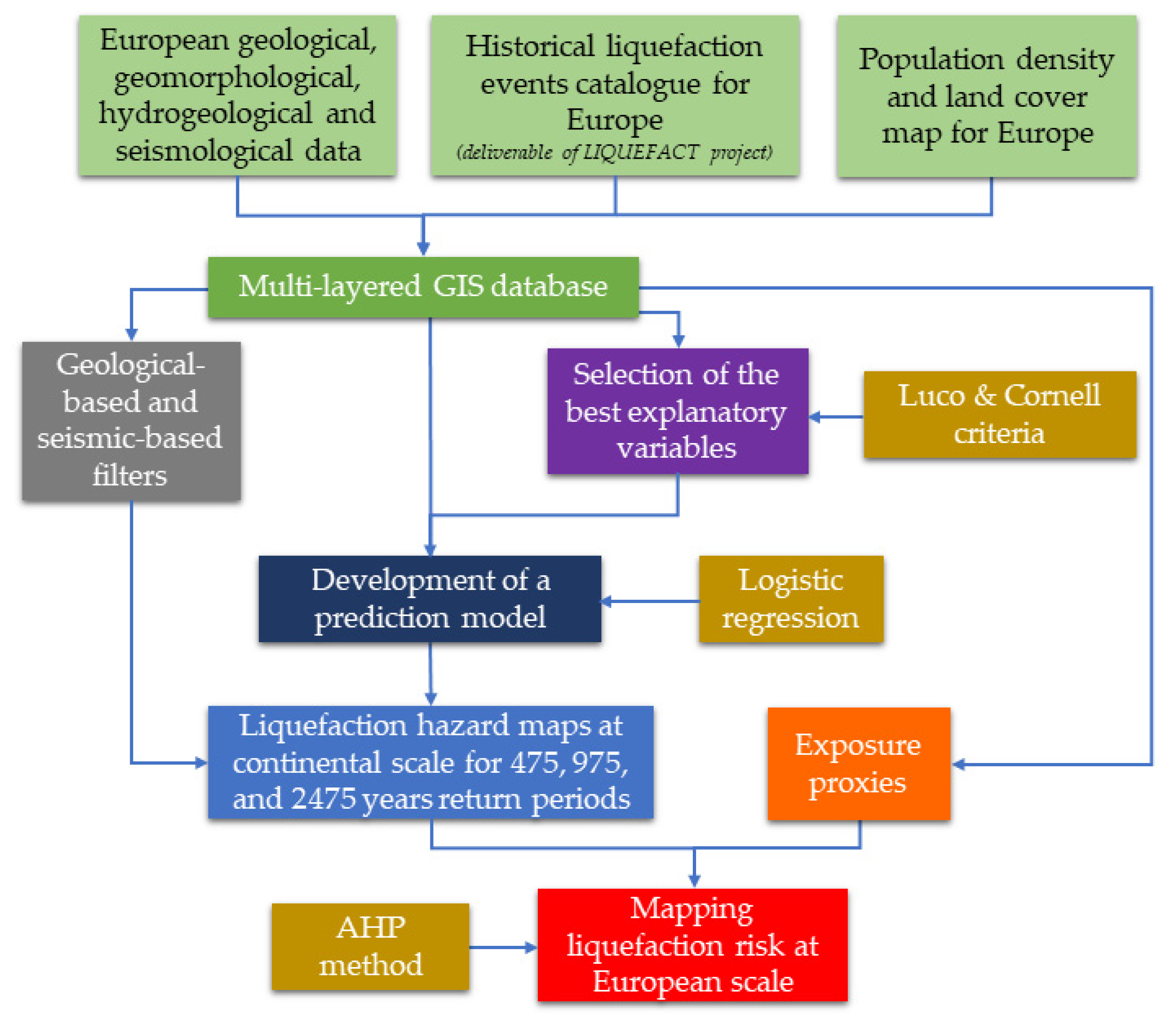
2. Overview of the Methodology

A geospatial methodology for zoning the earthquake-induced soil liquefaction risk at a continental scale was set-up in a GIS environment by coupling data-driven and knowledge-driven approaches. Figure 1 shows the flowchart including the main steps of the developed geospatial approach.
First, a multi-layered GIS database was built by harmonizing datasets available for the whole European territory, including the expected seismic hazard. European territories may not be susceptible to earthquake-induced liquefaction due to the geological setting and/or geotechnical characteristics [15] and/or they may be affected by a very low seismic hazard. Therefore, the liquefaction potential is a priori assumed negligible in these areas and a filter was applied in the mapping.
Moreover, a population density and land cover map from the CORINE initiative (https://land.copernicus.eu/pan-european/corine-land-cover) was adopted as proxy data for exposure at the European scale. The GIS database is fully accessible via the web through the Zenodo platform (https://zenodo.org/).
A data-driven prediction model based on a logistic regression was purposely developed for liquefaction occurrence in Europe using a set of optimal geospatial predictors, hereinafter also denoted as explanatory variables. The optimal explanatory variables were identified based on a well-established protocol proposed by Luco and Cornell [16,17,18]. To calibrate and successively validate the logistic regression, a database of liquefaction manifestations that occurred in continental Europe was used. These first steps of the methodology, herein briefly summarized, are fully described in Bozzoni et al. [7].
By applying the geospatial prediction model calibrated for Europe, the probability of liquefaction was mapped for the whole continent. Then, the AHP technique was used to identify areas that have a high risk of liquefaction by convolving seismic hazard, the susceptibility of soils to liquefaction, and exposure data. Indeed, the population density, a reasonable and well-established exposure indicator in urbanized territories, was combined with additional open-access exposure represented by the CORINE dataset, in order to provide the georeferenced distribution of strategic infrastructures in Europe.
Finally, the maps displaying the earthquake-related liquefaction risk were computed for different levels of severity of ground shaking specified by three return periods (i.e., 475, 975, and 2475 years).

3. Mega-Zonation of the Earthquake-Induced Liquefaction Risk in Continental Europe

The geospatial methodology presented in Section 2 was applied hereinafter for megazoning the earthquake-induced soil liquefaction risk in Europe. First, a European data-driven prediction model for liquefaction occurrence [7] was adopted for mapping the probability of liquefaction in the European territory (Section 3.1). Then, liquefaction potential charts were convolved with the exposure model adopted for Europe (Section 3.2) to assess the liquefaction risk at the continental scale. A knowledge-driven method was adopted at this stage. Indeed, the AHP technique was applied with the aim of mapping the liquefaction risk at the European scale, as illustrated in Section 3.3.

3.1. Mapping the Probability of Liquefaction by Applying A European Prediction Model

Geological, geomorphological, hydrogeological, and seismological information in addition to digital terrain and shallow lithology data available at the European scale were collected and processed in a GIS database with the final aim of mapping the liquefaction potential in Europe.
A prediction model was calibrated after constructing a dataset of liquefaction occurrences from four recent European earthquakes whose main characteristics (e.g., ground shaking maps, liquefaction manifestations) are well documented [7]. This dataset was adopted to identify the optimal explanatory variables best correlated with liquefaction occurrences. The last step was the calibration of the logistic regression model to predict liquefaction manifestations in both historical (for the validation of the model) and future earthquakes.
The optimal explanatory variables that, at a given point of the territory, are best correlated with liquefaction occurrence were identified according to the criteria of practicality, efficiency, and proficiency characterizing the Luco and Cornell methodology [16,17,18,19], which was originally developed for applications in structural earthquake engineering. Different explanatory variables were considered (e.g., the distance to the nearest river, to the nearest coast, and to the nearest water; the Terrain Roughness Index (TRI); and the Topographic Position Index (TPI). Three out of the nine explanatory variables were selected as optimal geospatial predictors of liquefaction occurrence [7]. They are listed as follows:
  • The weighted-mean shear-wave velocity in the top 30 m (VS30), which was adopted as a proxy of soil stiffness since soft sandy soils are more susceptible to liquefaction (they are looser). The US Geological Survey (https://earthquake.usgs.gov/data/vs30/) provided the global topographic-slope based VS30 map and such a map was adopted for Europe;
  • The Compound Topographic Index (CTI). The Digital Elevation Model (DEM) obtained from Shuttle Radar Topography Mission (SRTM) dataset [20] was processed to obtain the CTI [21];
  • The weighted-magnitude peak ground acceleration (PGAm), which was computed as
PGAm = PGA · MWF
where PGA are the values of peak ground acceleration (horizontal component), referred to three different return periods (475, 975, and 2475 years), for standard ground conditions (outcropping bedrock and level site), extracted from the deliverables of the SHARE project (Seismic hazard harmonization in Europe; http://www.share-eu.org/). These values of PGA were then multiplied by the soil factor defined in Eurocode 8 Part 1 [22] (hereinafter, EC8) to take into account the possible side effects. Ground categories of EC8 were assigned by exploiting the global topographic-slope-based VS30 map. In doing so, only 1D lithostratigraphic amplification was explicitly considered. MWF stands for Magnitude-Weighting Factor, which is defined by the following equation:
MWF =   Mw 2.56 10 2.24
where Mw was defined by using the European seismogenic zoning proposed in the SHARE project. The MWF [23] is the inverse of the Magnitude-Scaling Factor (MSF). Indeed, MSF is typically used as a proxy for earthquake duration, which plays a key role in liquefaction occurrence. Different models are available in the literature to define the MSF. In this study, the model adopted is that proposed by Youd et al. (2001) [24].
As mentioned above, the optimal geospatial explanatory variables were used to calibrate a data-driven model to predict liquefaction occurrence. For this purpose, logistic regression was applied to model the liquefaction occurrence in Europe based on recent studies in the literature [2,3,4]. Logistic regression is a machine learning procedure that is effective when analyzing a dataset in which several independent (explanatory) variables determine a binary outcome. In this case, the outcome is represented by a liquefaction label: 1 stands for liquefaction, 0 stands for no liquefaction. The independent variables are the geospatial explanatory proxies selected with the Luco and Cornell methodology, namely CTI, ln(PGAm) and ln(VS30). In the logistic regression, the probability of liquefaction is therefore calculated using the following equation:
P ( X )   =   1 1   +   e X
where X was computed as
X   =   γ 0   +   γ 1 x 1   +   γ 2 x 2   +     +   γ k x k
where the xk are the explanatory variables and γk the coefficients of the regression. By integrating the optimal geospatial predictors into Equation (4), the latter can be rewritten as follows:
X   =   A   +   B   ·   ln ( PGAm )   +   C   ·   CTI   +   D   ·   ln ( V S 30 )
The calibration of the coefficients A, B, C, and D of the regression was carried out using the previously mentioned dataset of liquefaction occurrences associated with the four European earthquakes, balanced after applying different sampling techniques. Indeed, three alternative re-sampling algorithms were adopted to correct the disproportion in the dataset of the size of the classes 1 and 0 of the cells. They are the under-sampling technique [25], the Synthetic Minority Over-Sampling Technique (SMOTE) [26], and the Adaptive Synthetic (ADASYN) [27] algorithms.
Each of these three re-sampling techniques was used to construct a different logistic prediction model for Europe. To calibrate the coefficients of the logistic regression the balanced dataset was split into two subsets: a training dataset and a testing dataset. In each of these two data groups, one out of two ratios between classes was maintained. The training dataset, including 75% of the balanced dataset, contained the cells upon which the coefficients of the prediction model were calibrated. On the other hand, the testing dataset contained data that were used to test the performance of the model in predicting liquefaction occurrence in historical earthquakes.
The goodness of the predictions of the alternative models was assessed quantitatively through a Receiver Operating Characteristics (ROC) analysis and expressed in terms of the parameter Area Under the Curve (AUC). The latter represents a useful procedure for organizing classifiers and visualize their performance, e.g., in Fawcett [28]. From ROC analysis applied to the training set, it turned out that the best prediction model of liquefaction occurrence is that associated with the ADASYN algorithm although the under-sampling and the SMOTE algorithms showed good performance as well [7].
After calibration of the coefficients, Equation (5) can be rewritten as follows:
X   =   11.489   +   3.864 ·   ln ( PGAm )   +   2.328 ·   CTI   +   0.091 ·   ln ( V S 30 )
Further details on the prediction model adopted for mapping the probability of liquefaction in Europe are discussed in the article by Bozzoni et al. [7]. The latter also computed liquefaction potential charts for continental Europe with reference to three levels of severity of the expected ground motion, namely for a seismic hazard with return periods of 475, 975, and 2475 years. The outcomes of this work were validated by superimposing on the charts the historical liquefaction cases from the European catalogue, delivered in the LIQUEFACT project. The charts of Figure 2a,b show the mega-zonation of European territory for liquefaction potential with reference to a return period of 475 years, superimposed on the locations of historical liquefaction occurrences associated with the same return period increased and decreased by +/− 10% [7]. It is important to remark that the latter are independent data with respect to the ones used to calibrate the prediction model. In the map, almost all the historical liquefaction manifestations are located in areas characterized by liquefaction potential (red areas in Figure 2a). This is particularly evident in Italy and the Balkan region. The results are also displayed in Figure 2b according to a chromatic scale based on the following five different classes of probability of liquefaction PL defined by Zhu et al. [2]: PL < 0.01 very low, 0.01 < PL < 0.03 low, 0.03 < PL < 0.08 medium, 0.08 < PL < 0.2 high, 0.2 < PL < 1 very high. It is worth noting that the historical liquefaction occurrences are mainly located in areas characterized by a very high probability of liquefaction.
It is important to remark that the liquefaction potential maps were computed in Bozzoni et al. [7] by pre-filtering the datasets in order to exclude from the analysis the territories that were either geologically incompatible with the phenomenon of earthquake-induced liquefaction (e.g., rocky formations) or characterized by an expected severity of ground shaking too low for liquefaction triggering (a value of horizontal peak ground acceleration equal to 0.1 g was arbitrarily assumed as a threshold in this regard).

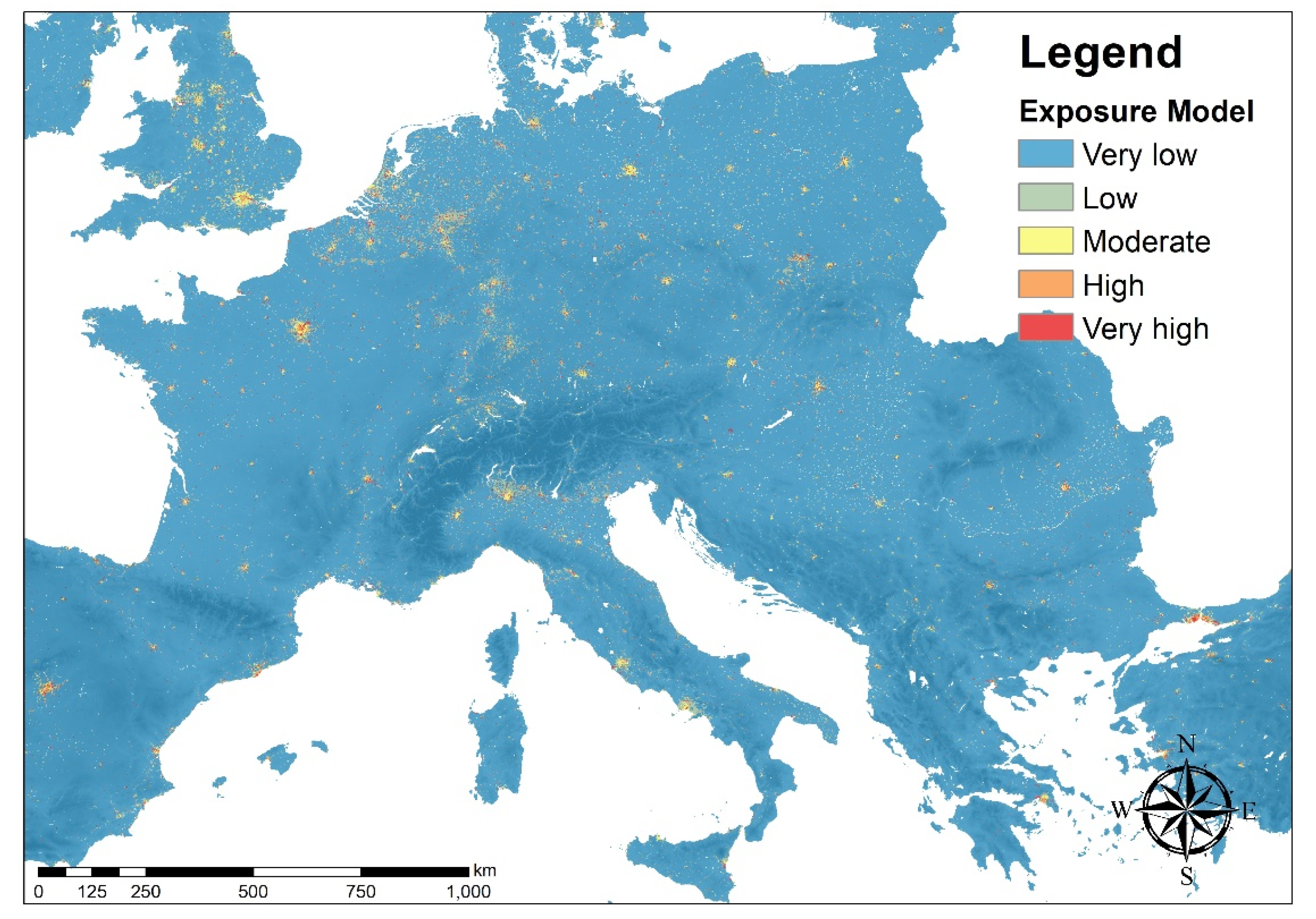
3.2. Exposure Model for Europe

Two indicators were used to account for the exposure in the computation of the risk maps. The population density, which is a well-established proxy in the case of urbanized territories [29], was combined with the CORINE land cover map for Europe which provides the geo-referenced distribution of non-residential, strategic areas in Europe.
The population density data for Europe was obtained from the European Global Human Settlement Layer (GHSL; https://ghsl.jrc.ec.europa.eu/index.php). The census data refer to the year 2015, and two different resolutions are available, 250 m and 1 km. The data are provided in a raster format, in which each cell contains the estimated number of inhabitants in that cell. The resolution adopted for this study was 1 km to be consistent with the resolution of the previously presented hazard charts. The raster map represents the population density in terms of inhabitants/km2 unit, which is the most common format to express the population density. The data were grouped into five classes of exposure, as done for the probability of liquefaction in Section 3.1. In particular, the following classes for the population density (Pd) were adopted:
  • very low: Pd < 400 inhab./km2;
  • low: 400 ≤ Pd 800 inhab./km2;
  • medium: 800 ≤ Pd < 2000 inhab./km2;
  • high: 2000 ≤ Pd < 5000 inhab./km2;
  • very high: Pd ≥ 5000 inhab./km2.
An additional proxy for exposure was found in the CORINE European map (http://land.copernicus.eu/pan-european/corine-land-cover/clc-2012/view), which provides the geo-referenced inventory on land cover areas in Europe. The data that referred to the land use was particularly helpful in order to identify strategic areas that population density could not identify.
Thus, the population density and the CORINE land cover were jointly adopted as exposure proxies. In particular, areas where airports, ports, roads, and railways are located across Europe were assigned to the highest exposure class (very high). The final exposure model is shown in Figure 3.

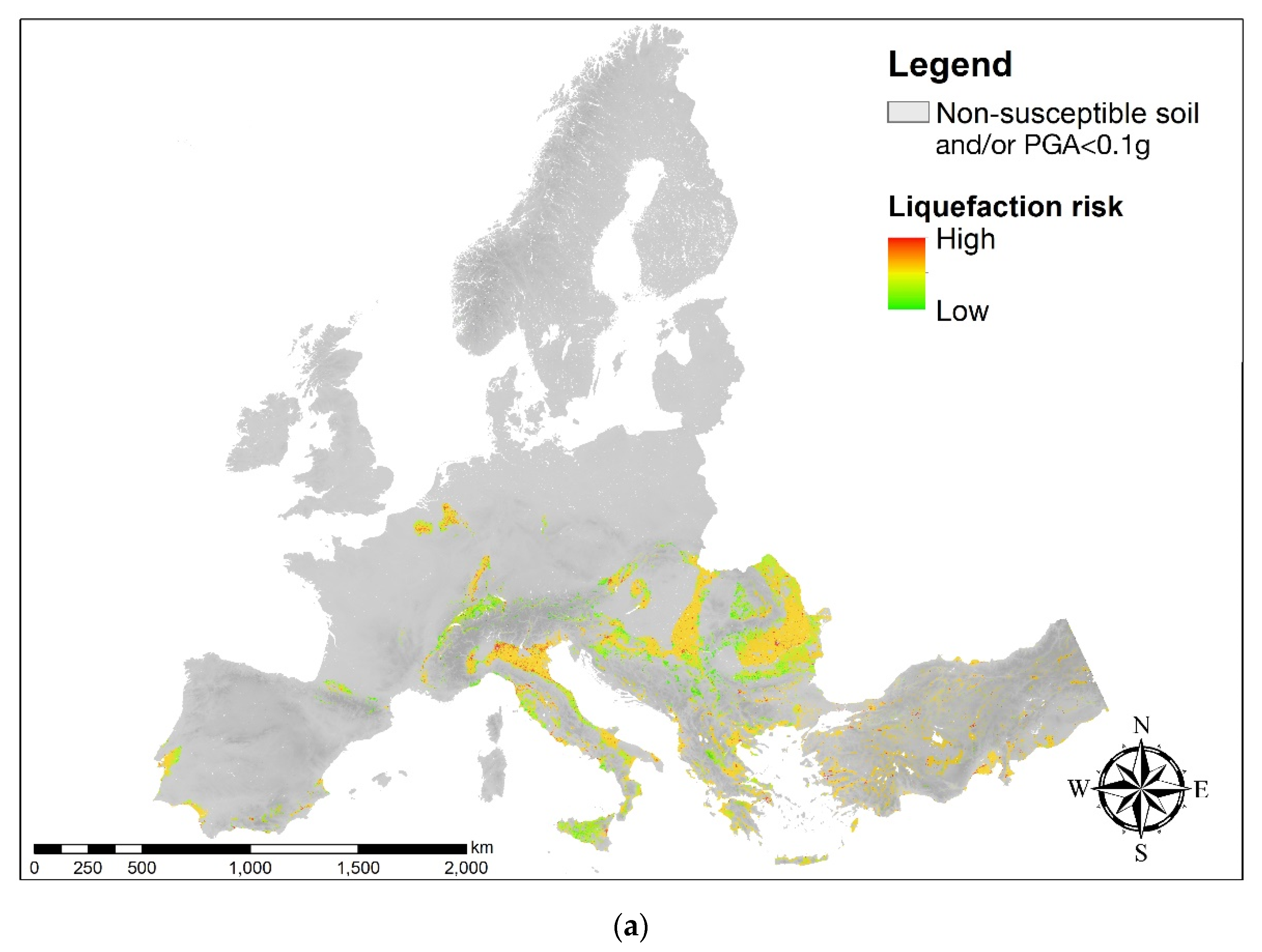
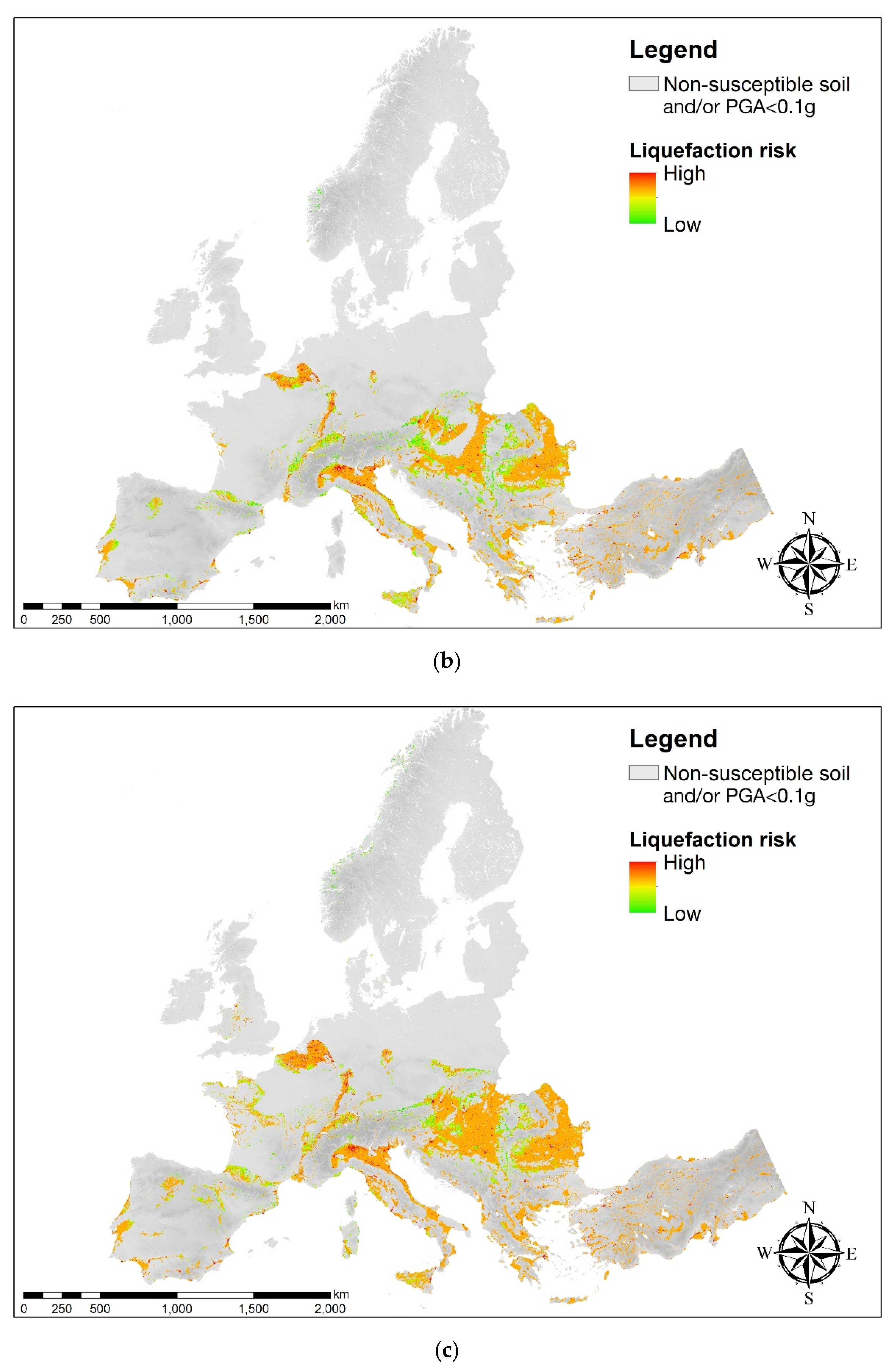
3.3. Assessment of the Liquefaction Risk at the European Scale by Using the AHP Technique

Since the risk of occurrence of earthquake-induced liquefaction is the convolution of seismic hazard, vulnerability, and exposure, the charts of liquefaction risk for Europe have been calculated by convolving these three variables represented as geospatial data at a continental scale. The risk assessment was carried out using the Analytical Hierarchy Process (AHP), a multi-criteria decision method introduced by Saaty [8] and then successfully applied for mapping natural hazards by [9,10,11]. The AHP technique belongs to the category of knowledge-driven methods. Indeed, a set of explanatory variables were ranked. Next, their relative importance was assessed with respect to the goal of the mapping by assigning weights via a pairwise comparison matrix. The final risk map was calculated based on weighted sums and rating assignments through a sequence of overlay operations. The assigned ranking was based on expert-judgment. The geospatial explanatory variables representing hazard, vulnerability, and exposure were combined, and the goal, with respect to which the variables were compared, was the liquefaction risk map. The more a variable influences the risk, the higher will be its weight in the calculation of the final chart. The main steps of AHP method procedure are explained hereinafter.
In Step 1, the alternatives were arranged in a GIS environment and their values were classified into different classes. The classes were ranked, from the highest class (i.e., the value that has the greatest importance for the goal of the map) to the lowest. Step 2 of the procedure involved organizing the data in a matrix. The pairwise comparison of the alternatives was carried out on a qualitative scale. Experts rated the comparison as equal, marginally strong, strong, very strong, and extremely strong, as shown in Table 1. As an example, the row corresponding to alternative A in the column corresponding to alternative B shows the value 9, indicating that A is “extremely strong” compared to B in light of the objective. In general terms, the alternatives in the ith row are stronger than those in the jth column if the value of the matrix (i, j) is greater than 1; otherwise, the alternatives in the jth column are stronger than those in the ith row. Consequently, the [j, i] element of the comparison matrix is the reciprocal of the [i, j] element.
Step 3 focused on the computation of the principal eigenvalue and the corresponding normalized right eigenvector of the comparison matrix built in Step 2. The elements of the normalized eigenvector were termed weights with respect to the goal of the map and the comparison of the alternatives. Step 4 involved an assessment of the consistency of the comparison matrix. Indeed, the AHP incorporates an effective technique for checking the consistency of the evaluations made by the decision-maker when building each of the pairwise comparison matrices involved in the process. A consistency index needed to be computed and, if it turned out that it was lower than a pre-defined threshold, the comparisons may have to be re-examined. The Consistency Index (CI) was then calculated by adopting the following relation:
CI = (λmax − n)⁄(n − 1)
where λmax is the maximum eigenvalue of the judgement matrix and n is the rank of the matrix. CI is then compared with that of a Random Matrix (RI). The corresponding ratio, i.e., CI/RI, is termed the Consistency Ratio (CR). Saaty [8] suggested that the upper threshold value of CR should be 0.1.
In the final step, namely, Step 5, the value of each alternative was multiplied by its own weight. Subsequently, the values obtained were summed up and the final rank calculated. This last step is developed in a GIS environment. The alternatives were represented by overlapped raster files: every pixel of each raster contains a value calculated in the first step. The final raster file consists of a map representing in each pixel the sum of the value contained in the pixels of the alternatives.

3.4. European Charts for Earthquake-Induced Liquefaction Risk

The AHP technique was applied following the steps of the procedure discussed in Section 3.3 with the aim of mapping the liquefaction risk at the European scale. Indeed, the probability of liquefaction computed for continental Europe (Section 3.2), was combined with the exposure model presented in Section 3.3. It is important to remark that a weight of 0.75 was assigned to the liquefaction potential, while a weight of 0.25 was assigned to exposure.
The earthquake-induced liquefaction risk charts computed for continental Europe with reference to three return periods (i.e., 475, 975, and 2475 years), are shown in Figure 4 (i.e., a, b, and c, respectively). The risk level is displayed by means of a chromatic scale, ranging from green (low level) to red (high level). The grey areas are a priori excluded because of the geological-based and seismic-hazard based filters applied.

4. Discussion and Concluding Remarks

In this article, a geospatial approach has been adopted for zoning the earthquake-induced soil liquefaction risk at the European scale (mega-zonation) for various return periods and taking into account exposure data. To the best of the authors’ knowledge, these are the first-ever produced maps of this kind. The few megazonation maps that exist in the literature on this subject address the susceptibility of soils to liquefaction and not the liquefaction risk using a probabilistic approach. In the procedure adopted in this study, geospatial data, machine learning, and knowledge-based algorithms were used to combine susceptibility of soil deposits to earthquake-induced liquefaction, seismic hazard, and exposure data so to yield probabilistic liquefaction risk maps of Europe.
The probability of liquefaction across this continent was mapped using logistic regression [7]. The analytical hierarchy process was then adopted to combine the liquefaction potential with an exposure model for Europe. The calculated maps referred to different levels of severity of ground shaking defined according to the European seismic hazard model delivered in 2013 within the SHARE project. An updated seismic hazard model for Europe is scheduled to be released at the beginning of 2021. When this happens or when other geospatial datasets such as the Vs30 or the exposure models are upgraded, the charts presented in this article will be recalculated—at least, this is the intention of the co-authors.
Liquefaction is an extremely local phenomenon of ground instability and mapping the liquefaction risk over a very large territory may sound like an oxymoron. In fact, the spatial resolution of the proposed charts is on the order of ~1 km, and as such, their level of accuracy is low. Yet, the availability of European charts of earthquake-induced liquefaction risk may still be valuable despite all their limitations. Indeed, they may be used to support decision-makers, civil protection agencies, insurance, and re-insurance companies to fund macro- (national scale), meso- (regional scale), and micro- (urban/sub-urban scale) zonation projects for detailed studies aimed to characterize a territory of smaller extension for liquefaction risk and the intrinsic vulnerability of the exposed assets.

Author Contributions

Methodology, F.B.; Formal analysis, D.C.; Supervision, C.G.L.; Data curation, R.B. and C.M.; Writing—original draft, F.B.; Writing—review & editing, R.B., Claudia Meisina, C.G.L. and E.Z.; Funding acquisition, F.B., C.M. and C.G.L. All authors have read and agreed to the published version of the manuscript.

Funding

This research has been carried out within the framework of the European LIQUEFACT project. The LIQUEFACT project received funding from the European Union’s Horizon 2020 Research and Innovation Programme under Grant Agreement No. 700748. This support is gratefully acknowledged by the authors.

Institutional Review Board Statement

Not applicable.

Informed Consent Statement

Not applicable.

Data Availability Statement

The GIS database herein presented is accessible via the web through the Zenodo platform (https://zenodo.org/).

Conflicts of Interest

The authors declare no conflict of interest.

References

  1. National Academies of Sciences, Engineering, and Medicine. State of the Art and Practice in the Assessment of Earthquake-Induced Soil Liquefaction and Its Consequences; The National Academies Press: Washington, DC, USA, 2016. [Google Scholar] [CrossRef]
  2. Zhu, J.; Daley, D.; Baise, L.; Thompson, E.; Wald, D.; Knudsen, K. A Geospatial Liquefaction Model for Rapid Response and Loss Estimation. Earthq. Spectra 2015, 31, 1813–1837. [Google Scholar] [CrossRef]
  3. Matsuoka, M.; Wakamatsu, K.; Hashimoto, M.; Senna, S.; Midorikawa, S. Evaluation of liquefaction potential for large areas based on geomorphologic classification. Earthq. Spectra 2015, 31, 2375–2395. [Google Scholar] [CrossRef]
  4. Zhu, J.; Baise, L.; Thompson, E. An Updated Geospatial Liquefaction Model for Global Application. Bull. Seismol. Soc. Am. 2017, 107, 1365–1385. [Google Scholar] [CrossRef]
  5. Rashidian, V.; Baise, L.G. Regional efficacy of a global geospatial liquefaction model. Eng. Geol. 2020, 272. [Google Scholar] [CrossRef]
  6. Yilmaz, C.; Silva, V.; Weatherill, G. Probabilistic framework for regional loss assessment due to earthquake-induced liquefaction including epistemic uncertainty. Soil Dyn. Earthq. Eng. 2020, in press. [Google Scholar] [CrossRef]
  7. Bozzoni, F.; Bonì, R.; Conca, D.; Lai, C.G.; Zuccolo, E.; Meisina, C. Megazonation of earthquake-induced soil liquefaction hazard in continental Europe. Bull. Earthq. Eng. 2020, in press. [Google Scholar] [CrossRef]
  8. Saaty, T.L. The Analytic Hierarchy Process; McGraw-Hill: New York, NY, USA, 1980. [Google Scholar]
  9. Karimzadeh, S.; Miyajima, M.; Hassanzadeh, R.; Amiraslanzadeh, R.; Kamel, B. A GIS-based seismic hazard, building vulnerability and human loss assessment for the earthquake scenario in Tabriz. Soil Dyn. Earthq. Eng. 2014, 66, 263–280. [Google Scholar] [CrossRef]
  10. Panahi, M.; Rezaie, F.; Meshkani, S. Seismic vulnerability assessment of school buildings in Tehran city based on AHP and GIS. Nat. Hazards Earth Syst. Sci. 2015, 15, 461–474. [Google Scholar] [CrossRef] [Green Version]
  11. Moustafa, S.S.R. Application of the Analytic Hierarchy Process for Evaluating Geo-Hazards in the Greater Cairo Area, Egypt. Electron. J. Geotech. Eng. 2015, 20, 1921–1938. Available online: http://www.ejge.com/2015/Ppr2015.0207sb.pdf (accessed on 18 December 2020).
  12. Lai, C.G.; Conca, D.; Bozzoni, F.; Bonì, R.; Meisina, C. Earthquake-induced soil liquefaction risk: Macrozonation of the European territory taking into account exposure. In Proceedings of the IABSE Symposium 2019 Guimarães. Towards a Resilient Built Environment—Risk and Asset Management, Guimarães, Portugal, 27–29 March 2019. [Google Scholar]
  13. UNESCO. Report of Consultative Meeting of Experts on the Statistical Study of Natural Hazards and Their Consequences; United Nations Educational Scientific and Cultural Organizations Document SC/WS/500; UNESCO: Paris, France, 1972. [Google Scholar]
  14. Lai, C.G.; Meisina, C.; Bozzoni, F.; Conca, D.; Bonì, R. Report to Describe the Adopted Procedure for the Development of the European Liquefaction Potential Map; Deliverable D2.6. V 1.0. Liquefact Project, H2020-DRA-2015, GA No. 700748; 2019; Available online: http://www.liquefact.eu/wp-content/uploads/2020/03/D2.6.pdf (accessed on 18 December 2020).
  15. Meisina, C.; Bonì, R.; Bozzoni, F.; Conca, D.; Perotti, C.; Persichillo, P.; Lai, C.G. Assessment of the soil liquefaction susceptibility across Europe using Analytic Hierarchy Process (AHP). Eng. Geol. 2020, submitted. [Google Scholar]
  16. Cornell, C.A.; Luco, N. Ground motion intensity measures for structural performance assessment at near-fault sites. In Proceedings of the Proceedings U.S.-Japan Joint Workshop and Third Grantees Meeting, Seattle, WA, USA, 15–16 August 2001. [Google Scholar]
  17. Luco, N.; Cornell, C.A. Structure-specific scalar intensity measures for near-source and ordinary earthquake ground motions. Earthq. Spectra 2007, 23, 357–392. [Google Scholar] [CrossRef] [Green Version]
  18. Padgett, J.E.; Nielson, B.G.; DesRoches, R. Selection of optimal intensity measures in probabilistic seismic demand models of highway bridge portfolios. Earthq. Eng. Struct. Dyn. 2008, 37, 711–725. [Google Scholar] [CrossRef]
  19. Wang, X.; Shafieezadeh, A.; Ye, A. Optimal intensity measures for probabilistic seismic demand modeling of extended pile-shaft-supported bridges in liquefied and laterally spreading ground. Bullettin Earthq. Eng. 2018, 16, 229–257. [Google Scholar] [CrossRef]
  20. Jarvis, A.; Reuter, H.I.; Nelson, A.; Guevara, E. Hole-Filled SRTM for the Globe. Version 4. 2008. Available online: http://srtm.csi.cgiar.org (accessed on 18 December 2020).
  21. Beven, K.J.; Kirkby, M.J. A physically based, variable contributing area model of basin hydrology. Hydrol. Sci. Bull. 1979, 24, 43–69. [Google Scholar] [CrossRef] [Green Version]
  22. Eurocode 8. Design of Structures for Earthquake Resistance, Part 1: General Rules, Seismic Actions and Rules for Buildings; Pr-EN1998-1; European Committee for Standardization (CEN): Brussels, Belgium, 2004.
  23. Chen, R.; Harmsen, S. Probabilistic Ground Motion Calculations and Implementation of PGA Scaling by Magnitude for Assessing Liquefaction Potential, Technical Document 2012-1, Seismic Hazard Zonation Program. 2012.
  24. Youd, T.L.; Idriss, I.M.; Andrus, R.D.; Arango, I.; Castro, G.; Christian, J.T.; Dobry, R.; Finn, W.D.L.; Harder, L.F.; Hynes, M.E.; et al. Liquefaction resistance of soils: Summary report from the 1996. NCEER and 1998 NCEER/NSF workshops on the evaluation of liquefaction resistance of soils. J. Geotech. Geoenviron. Eng. 2001, 127, 817–833. [Google Scholar] [CrossRef] [Green Version]
  25. Yen, S.J.; Lee, Y.S. Under-Sampling Approaches for Improving Prediction of the Minority Class in an Imbalanced Dataset. In Intelligent Control and Automation. Lecture Notes in Control and Information Sciences; Huang, D.S., Li, K., Irwin, G.W., Eds.; Springer: Berlin/Heidelberg, Germany, 2006; Volume 344. [Google Scholar] [CrossRef]
  26. Chawla, N.V.; Bowyer, K.W.; Hall, L.O.; Kegelmeyer, W.P. SMOTE: Synthetic Minority Over-sampling Technique. J. Artif. Intell. Res. 2002, 16, 321–357. [Google Scholar] [CrossRef]
  27. He, H.; Bai, Y.; Garcia, E.A.; Li, S. ADASYN: Adaptive Synthetic Sampling Approach for Imbalanced Learning. In Proceedings of the 2008 IEEE International Joint Conference on Neural Networks (IEEE World Congress on Computational Intelligence), Hong Kong, China, 1–8 October 2008. [Google Scholar]
  28. Fawcett, T. An introduction to ROC analysis. Pattern Recognit. Lett. 2005, 27, 861–874. [Google Scholar] [CrossRef]
  29. Sousa, L.; Silva, V.; Bazzurro, P. Using Open-Access Data in the Development of Exposure Data Sets of Industrial Buildings for Earthquake Risk Modeling. Earthq. Spectra 2017, 33, 63–84. [Google Scholar] [CrossRef]
Figure 1. Flowchart of the geospatial approach developed in this study for mapping the liquefaction risk at a continental scale.
Geosciences 11 00032 g001
Figure 2. Maps showing the liquefaction potential for the European territory referred to the return period of 475 years [7]. The results are expressed (a) as a binary outcome, i.e., liquefaction or no liquefaction, and (b) according to a chromatic scale based on five different classes of the probability of liquefaction. Locations of liquefaction occurrences (black dots) associated with a return period of about 475 years are superimposed to both charts. The grey areas are a priori excluded because of either the geological-based or the seismic-hazard based filters herein applied (the greyscale is based on Digital Elevation Model, DEM).
Geosciences 11 00032 g002
Figure 3. Exposure model for Europe adopted in this study by combining open-access data on population density and land cover in Europe, used as proxies for urbanized areas and strategic infrastructures, respectively.
Geosciences 11 00032 g003
Figure 4. European liquefaction risk maps were calculated in this study for the return periods of 475 (a), 975 (b), and 2475 (c) years. The grey areas are a priori excluded because of the geological-based and seismic-hazard based filters applied (the greyscale is based on the DEM).
Geosciences 11 00032 g004aGeosciences 11 00032 g004b
Table 1. Application of Analytical Hierarchy Process (AHP) method: relative importance for comparison between different alternatives [8].
Weight/RankRelative Importance
1equal
3moderately dominant
5strongly dominant
7very strongly dominant
9extremely dominant
2, 4, 6, 8intermediate values
Reciprocalsfor inverse judgements
Publisher’s Note: MDPI stays neutral with regard to jurisdictional claims in published maps and institutional affiliations.

