Regional Analyses of Rainfall-Induced Landslide Initiation in Upper Gudbrandsdalen (South-Eastern Norway) Using TRIGRS Model

Abstract

In Norway, shallow landslides are generally triggered by intense rainfall and/or snowmelt events. However, the interaction of hydrometeorological processes (e.g., precipitation and snowmelt) acting at different time scales, and the local variations of the terrain conditions (e.g., thickness of the surficial cover) are complex and often unknown. With the aim of better defining the triggering conditions of shallow landslides at a regional scale we used the physically based model TRIGRS (Transient Rainfall Infiltration and Grid-based Regional Slope stability) in an area located in upper Gudbrandsdalen valley in South-Eastern Norway. We performed numerical simulations to reconstruct two scenarios that triggered many landslides in the study area on 10 June 2011 and 22 May 2013. A large part of the work was dedicated to the parameterization of the numerical model. The initial soil-hydraulic conditions and the spatial variation of the surficial cover thickness have been evaluated applying different methods. To fully evaluate the accuracy of the model, ROC (Receiver Operating Characteristic) curves have been obtained comparing the safety factor maps with the source areas in the two periods of analysis. The results of the numerical simulations show the high susceptibility of the study area to the occurrence of shallow landslides and emphasize the importance of a proper model calibration for improving the reliability.

1. Introduction

The study of rainfall-induced landslides is an important research topic for the improvement of risk mitigation strategies for current and future climate scenarios. For this reason, over the years a number of solutions have been developed on this issue, often based on statistical-probabilistic techniques (e.g., [1,2,3,4]). However, even though these methods can be very effective in the identification of the areas more prone to slope failure (i.e., landslide susceptibility), the same cannot be said about the temporal prediction of such phenomena, which still represents a challenging research topic. In this respect, also considering the improvements of environmental sensing technology, different landslide early warning systems (LEWSs) have been recently drawn up, both at slope scale (see [5] and references therein) and over national/regional scale (see [6] and references therein), such as the one developed. These systems basically monitor the most significant variables related to the triggering conditions (e.g., rainfall, soil moisture, displacement) and, when given thresholds are exceeded, warning messages are generated to alert the public and authorities [7]. Every early warning system operational worldwide has a different number of thresholds and algorithms to activate a warning level. Such thresholds can be defined using different tools, including physically based models that reproduce, often via numerical simulations, the progressive onset of the instability within the potentially unstable soil during heavy rainfall events (e.g., [8,9,10,11]). However, a correct spatial evaluation of the input parameters (e.g., rainfall field, initial water table, thickness and physical–mechanical parameters of the soil cover) is a fundamental aspect for the reliable application of such models. In this respect, back-analyses of preceding landslide events is a common strategy to calibrate the inputs parameters of physically based models.

The results presented in this paper have been obtained applying the physically based model TRIGRS [12], which is a model specifically devoted to the prediction of rainfall-induced landslides. Since the model calculates the slope stability conditions in response to specific rainfall events, we have back-analysed two separate landslide events that occurred in the upper Gudbrandsdalen, Eastern Norway, on 10 June 2011 and 22 May 2013 [13]. The unstable areas obtained by the application of TRIGRS (Safety Factor lower than 1) have been compared with the source areas observed in situ. The outcome of this comparison was then evaluated through a ROC (receiver operating characteristic) curve analysis, allowing is to quantify the performance of the two predictions.

2. Materials and Methods

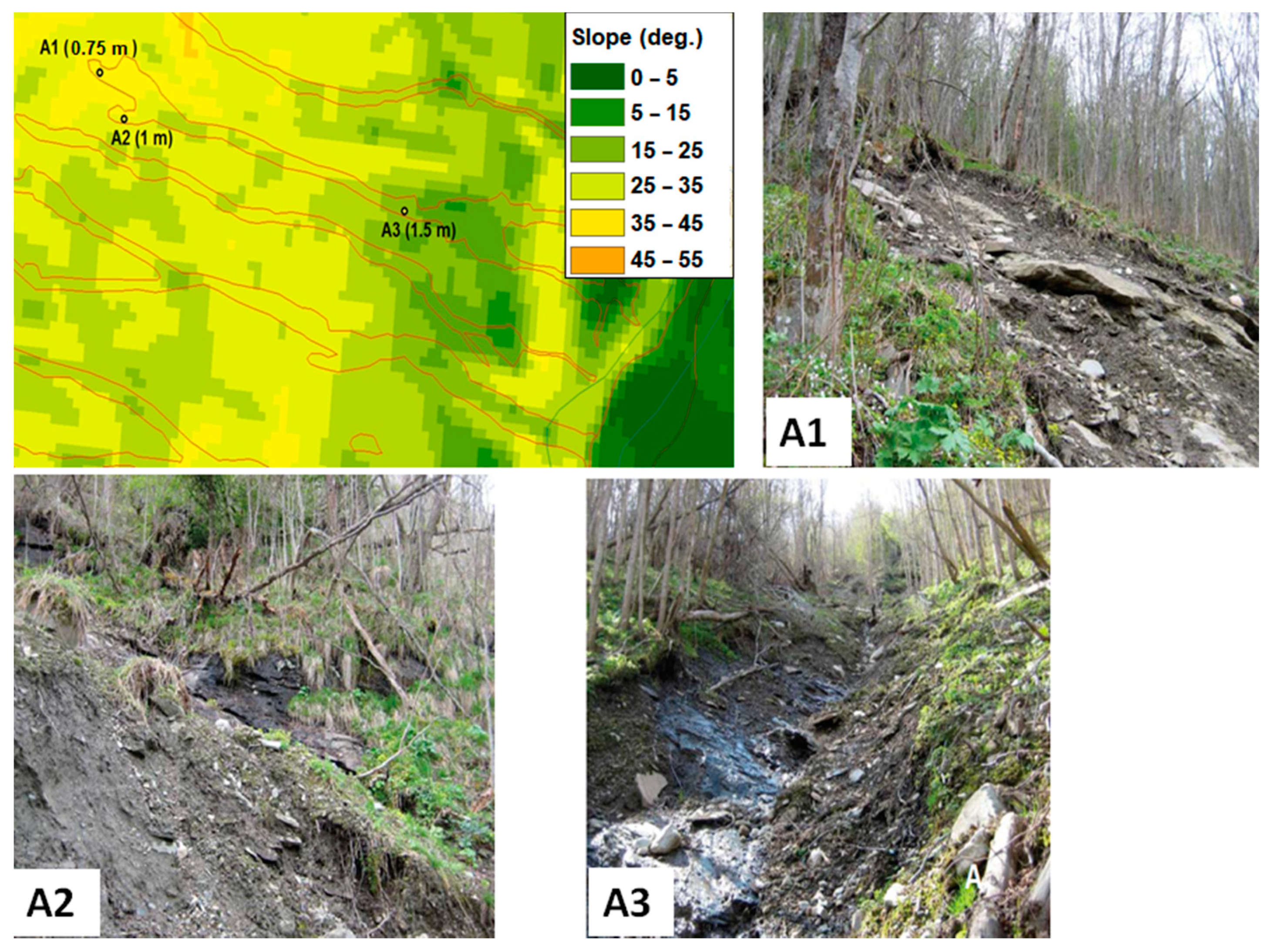
2.1. The Case Study

Gudbrandsdalen is a major north–south trending valley in the mountainous part of the former Oppland county (now Innlandet county) in South-Eastern Norway (Figure 1). Specifically, the study area (Veikledalen) is in the upper part of this region, near the village of Kvam. The area is characterized by hill slopes mainly consisting of green or grey phyllite, within which layers of grey sandstone, feldspathic sandstone or quartzite can be found [14]. These slopes have been largely carved by glaciers, whose erosive action is also testified by the presence of till deposits of variable thickness. In general, the thinner deposits (0.5 m or less) are in the upper part of the slopes, while in the lower parts, the thickness can reach several tens of meters. The valley floor is mainly filled by glacifluvial and fluvial deposits, which can be locally covered by Holocene colluvial fans generated at the toe of the numerous gullies cutting the till deposits [15]. In this respect, the area has experienced different landslide events recently, mainly channelized debris flows generally initiated as shallow slides within the soil cover (i.e., soil slips). The most recent events occurred in May 2008, June 2011 and May 2013. In particular, the last two occurred in very similar hydrometeorological conditions that also triggered flood events along the Glomma river.

In the period 6–12 June 2011, significant rainfall occurred, and the simultaneous high temperature led to strong snow-melting process. Due to such a combined effect, several shallow landslides were triggered in the night between the 9 and 10 June, causing the closure of numerous roads in Gudbrandsdalen. More than 270 people were evacuated, and the overall damages cost is estimated at 800 million Norwegian Kroner (NOK), ca. 100 million USD. On 22 May 2013, the combination of intense rainfall and prolongated, intense snow melting caused widespread flooding and many shallow landslides in the same area [13]. The worst damage was recorded in the town of Kvam, where more than 200 residents were evacuated. As in 2011, the two main roads, the National Highway Rv3 and the European highway E6, were closed at several locations. The damage cost is estimated at a total of 1500 million NOK, ca. 170 million EUR [16]. In this work, the over 100 landslides triggered during both events have been identified through the analysis of high-resolution aerial orthophotos by distinguishing, for each landslide, the source area from the propagation and deposition zones (Figure 2).

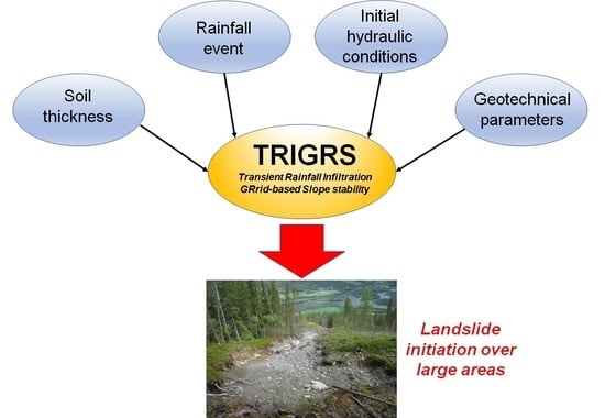
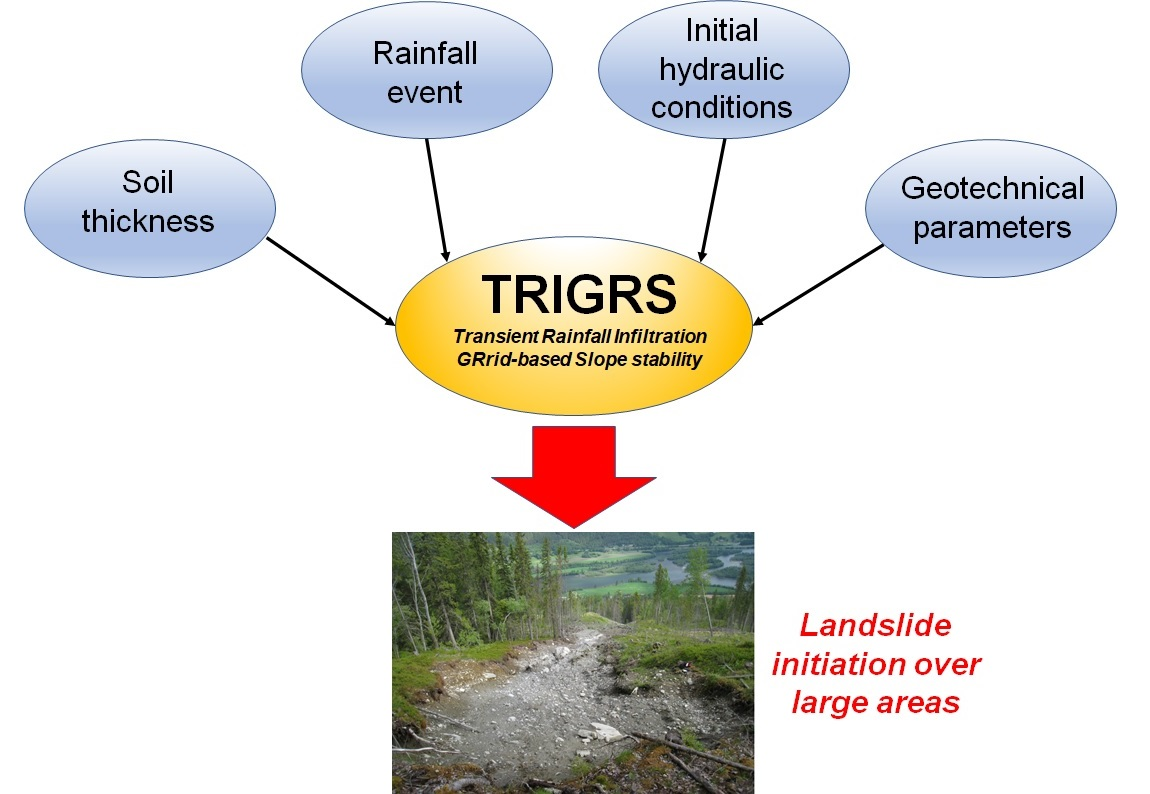
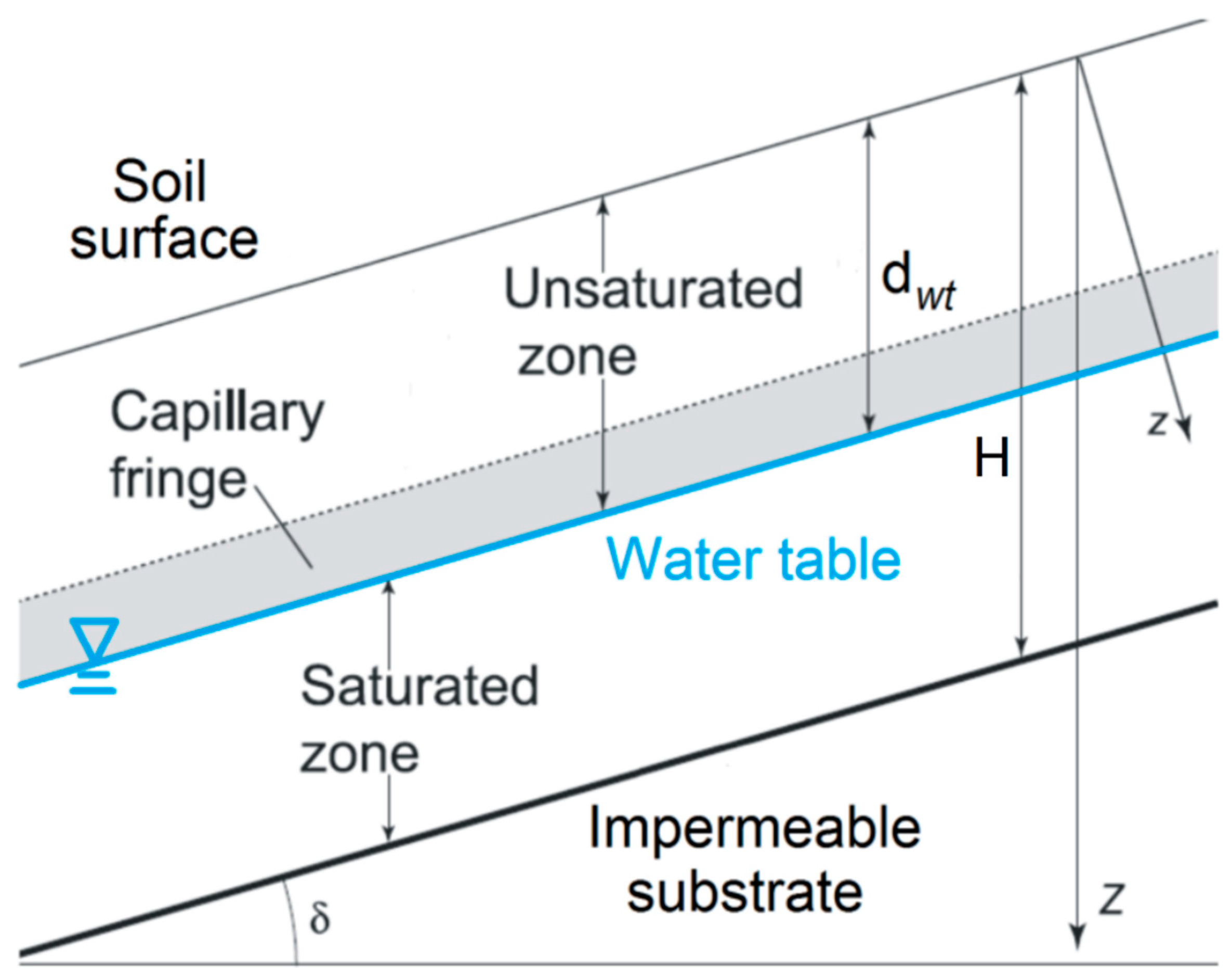
2.2. The TRIGRS Model

TRIGRS is a widely used numerical model in the framework of landslide susceptibility analyses (e.g., [17,18,19]). It can reproduce, in a simplified form, the triggering process of rainfall-induced shallow landslides considering relatively few and simple input parameters. Specifically, it performs a slope stability analysis over large areas through the infinite slope limit equilibrium method, considering a transient 1-D analytic solution for pore water pressure induced by rainfall infiltration based on [20] linearized solution of the Richards’ equation. In other words, it is possible to consider a space–time variability of rainfall input (I_Z) that, together with a simple runoff routing scheme, allows calculating the pressure head response ψ(Z, t) for each grid cell starting from initial saturated or unsaturated conditions. In this latter case, the model uses a simple analytic solution proposed by [21] to linearize the Richards’ equation, considering four hydrodynamic parameters: the saturated (θ_s) and residual (θ_r) water content, the saturated hydraulic conductivity (K_s) and a specific parameter linked to the pore size distribution (α_G). If the amount of infiltrating water reaching the water table exceeds the maximum amount that can be drained by gravity, TRIGRS simulates the water-table rise, comparing the exceeding water quantity to the available pore space directly above the water table or capillary fringe (Figure 3) and then, for each time step, it applies the water weight at the initial top of the saturated zone to compute the new pressure head [22]. For the calculation of the safety factor in the unsaturated configuration, the pressure head is multiplied by the effective stress parameter χ, as suggested by [23]:

χ = (θ − θ_r)/(θ_s − θ_r)

(1)

where θ is the soil water content. This approximation represents a simplified form of the suction–stress characteristic curve [24,25]. The Safety Factor at a specific depth Z is then calculated according to:

FS(Z,t) = (tanφ’/tanδ) + {[c’ − (ψ(Z,t) γ_w tanφ’)]/[γ Z sinδ cosδ]}

(2)

where δ is the slope angle, c’ is the effective soil cohesion, φ’ is the effective friction angle of the soil, γ_w is the unit weight of groundwater and γ is the total unit weight of soil. A more detail explanation of the assumptions, fundamental concepts and equation derivation of the TRIGRS model can be found in [12,22].

To calculate the Safety Factor in response to specific rainfall events, TRIGRS uses a series of input parameters (Table 1). Two different detailed (5 × 5 m) digital elevation models (DEM) are available for the study area. The first one was dated 2010, i.e., before the 2011 landslide event, and the second one was dated 2012. Considering this aspect, we decided to use the 2010 DEM for deriving the slope map of the area in the case of the 2011 event simulation, and the 2012 DEM for the 2013 event.

For the estimation of the spatial variation of the thickness of the surficial cover, a modified version of the model proposed by [26] has been applied to the study area. The original model correlates the soil depth to the local slope angle according to the following equation:

h_i = h_max {1 − {[(tanα_i − tanα_min)/(tanα_max − tanα_min)] [1 − (h_min/h_max)]}}

(3)

where α_i is the slope value at pixel i, while α_max and α_min are the maximum and minimum slope values encountered in the study area, h_i is the soil thickness computed at pixel i, h_max and h_min are the maximum and minimum soil thickness values measured in the area. However, Equation (3) was modified in such a way that a series of real thickness data deriving from different sources could be used, then improving the reliability of the model itself. The available data are summarized in

Table 2. Thickness data of the surficial cover available for the study area.

Type of Data	Points	Source
Field data–GPS position	3	[29]
Field data	4	[30]
Calculated data	36	LIDAR-based 1 × 1 m2 DEMs

.

Table 1. Input parameters for the TRIGRS model.

Parameter	Unit	Attributed Value	Source
Slope (δ)	(°)	Spatially variable	5 × 5 m DEM
Soil thickness (H)	(m)	Spatially variable	Fitting equation
Friction angle (φ’)	(°)	32	[27]
Cohesion (c’)	(kN m−2)	4	[27]
Soil unit weight (γ)	(kN m−3)	20	[27]
Hydraulic conductivity (Ks)	(m s−1)	1.0 × 10−5	[27]
Hydraulic diffusivity (D0)	(m2 s−1)	4.0 × 10−4	[27]
Saturated water content (θs)	(-)	0.45	ROSETTA Lite module
Residual water content (θr)	(-)	0.03	ROSETTA Lite module
Pore-size parameter (αG)	(m−1)	0.02	ROSETTA Lite module + [28]
Initial water table depth (dwt)	(m)	Spatially variable	Varsom Xgeo
Background rainfall rate (IZLT)	(m s−1)	Spatially variable	Varsom Xgeo
Rainfall rate (IZ)	(m s−1)	Spatially variable	Norwegian Meteorological Institute

Table 1. Input parameters for the TRIGRS model.

Parameter	Unit	Attributed Value	Source
Slope (δ)	(°)	Spatially variable	5 × 5 m DEM
Soil thickness (H)	(m)	Spatially variable	Fitting equation
Friction angle (φ’)	(°)	32	[27]
Cohesion (c’)	(kN m−2)	4	[27]
Soil unit weight (γ)	(kN m−3)	20	[27]
Hydraulic conductivity (Ks)	(m s−1)	1.0 × 10−5	[27]
Hydraulic diffusivity (D0)	(m2 s−1)	4.0 × 10−4	[27]
Saturated water content (θs)	(-)	0.45	ROSETTA Lite module
Residual water content (θr)	(-)	0.03	ROSETTA Lite module
Pore-size parameter (αG)	(m−1)	0.02	ROSETTA Lite module + [28]
Initial water table depth (dwt)	(m)	Spatially variable	Varsom Xgeo
Background rainfall rate (IZLT)	(m s−1)	Spatially variable	Varsom Xgeo
Rainfall rate (IZ)	(m s−1)	Spatially variable	Norwegian Meteorological Institute

The first dataset [29] is composed by measurements of the surficial cover thickness for which the GPS position is available from field surveys (Figure 4), whereas the second series of data are measurements whose position has been identified by using the information reported in [30]. Regarding the third dataset, we first identified from high-resolution aerial orthophotos 36 points within the footprint areas where the bedrock was clearly exposed after the landslide events. Then, we made the difference between two high-resolution (1 × 1 m) DEMs derived from LIDAR data (Figure 5). Since the DEMs had been released before (i.e., 2000) and after (i.e., 2012) the 2011 landslide event, it was possible to measure the effective thickness of the surficial cover in each of the 36 points. Afterwards, all the 43 thickness values (and the corresponding slope values measured in each point) were plotted in a graph “thickness vs. tangent of slope”, and a least squares linear fit of the points was used as the soil thickness model (Figure 6). It is important to note that for the numerical simulations we decided to neglect the areas with thickness values higher than 2 m in the lower part of the valley, since the real thickness of the surficial cover is considerably higher than the expected, and it could not be simplified with a linear trend. On the other end, we imposed a constant value of 0.4 m (i.e., the lowest thickness value measured on field) for the steepest areas. However, the thickness of the surficial cover also depends on the geological and geomorphological features of the area, which are those typical of glacial environments. In this respect, the map of the Quaternary deposits available at the Geological Survey of Norway (NGU) shows the presence of “shallow” glacial deposits in the upper part of the slopes, whereas the “thick” glacial deposits can be found only in the lower part of the valleys. Considering this last aspect, we decided to impose a constant value of 0.4 m in the areas characterized by the presence of shallow glacial deposits, and a null value for the areas where the bedrock outcrops.

As far as the geotechnical and hydraulic parameters of the debris cover are concerned, unfortunately no data deriving from laboratory or field tests are available for the study area, as well as in many other areas in Norway. Therefore, as a first step we decided to use the values reported in [27]. In this paper, the authors calibrated the soil parameter values through Monte Carlo simulations using as constraint a series of debris flows located near Otta, northwest of the study area. Specifically, starting from the spatial distribution of the Quaternary deposits, deriving from two maps at 1:20,000 and 1:50,000 scale, they perform numerical simulations by imposing as target the maximization and minimization of areas classified as unstable for a 1000-year return period rainfall event and in absence of precipitation, respectively. The resulting values related to the glacial deposits are reported in Table 1.

For the estimation of the hydrodynamic parameters employed by TRIGRS in the unsaturated modality, we used the ROSETTA Lite module [31] available within the HYDRUS-1D software [32]. This module uses a database of measured water retention and other properties for a wide variety of media. Specifically, for a given grain-size distribution the model estimates a soil water retention curve (SWRC) based on the hydraulic model proposed by [33] and with good statistical comparability to known retention curves of other media with similar physical properties [34]. In this work, an average grain size distribution has been considered according to four samples collected in the case study area [35]. However, the α_G parameter corresponds to a fitting parameter of the SWRC based on a different ([36] hydraulic model. This parameter was then estimated using the conversion formula from [28], which defines a correspondence between the above-mentioned hydraulic models through the capillary length approach [37].

The initial water-table depth and the background rainfall rate are, instead, closely related to the preceding hydrological conditions, which can highly affect the spatio-temporal occurrence of rainfall-induced landslides [38]. Such parameters were estimated from the information reported in Varsom Xgeo (www.xgeo.no). It is an open access decision-support tool developed from the cooperation between the Norwegian Water Resources and Energy Directorate (NVE) and other governmental agencies such as the Norwegian Meteorological Institute, the National Public Road Administration, the National Rail Administration and the National Mapping Authority. Specifically, it is composed of a web portal and several modules that store different types of data such as: gridded maps (spatial resolution: 1 km²) of meteorological data and simulated hydrological, glaciological and hydrogeological conditions; real-time data recorded at automatic stations; field observations (i.e., snow conditions, landslide events); thematic maps; warnings maps; and satellite images. The tool is daily employed for national forecasting and warning services (e.g., floods, landslides and snow avalanches) carried out by NVE over the entire national territory [39].

The hydrological conditions reported in Varsom Xgeo derive from simulations performed at the daily scale with HBV, which is a semi-distributed conceptual rainfall-runoff model [40,41]. Specifically, two versions of the model are daily employed at NVE: a river-catchment-type version that is calibrated over 150 river catchments and a spatially distributed-type version (also known as GWB-Gridded Water Balance). The latter version considers each of 385,000 cells over the entire Norwegian territory as a separate basin, for which a specific water balance is performed. The model runs 24 h a day and uses precipitation and air mean temperature as inputs. The main structure of the HBV model comprises four storage components: snow, soil moisture, and upper and lower runoff zone. The model can reproduce not only runoff, but also infiltration and snow melting, then estimating the corresponding variations of groundwater level, soil saturation, soil frost, etc. In particular, the groundwater-level map provides information on the groundwater level compared to the average for the same day for the reference period 1981–2010. The degree of soil-saturation map (Figure 7) shows the percentage of soil saturation, which describes the relationship between current soil-water storage compared to the maximum soil-water storage simulated with the HBV model in the reference period 1981–2010. In this work, the degree of soil saturation was used for the estimation of the background rainfall rate (I_ZLT). Such a parameter represents the steady (initial) surface flux, which can usually be approximated by the average precipitation in recent weeks or months that is needed to maintain the initial conditions [22]. However, information about methods for estimating I_ZLT is rare in the literature. If the soil is saturated, I_ZLT can be the same as hydraulic conductivity, while it can be zero for dry soil. For this reason, several authors [42,43,44,45] calculated this parameter as a fraction of the hydraulic conductivity considering the long-term weather conditions prior the investigated period. Thus, we spatially varied the background rainfall rate as a function of the degree of soil-saturation map available for both the events: the higher the degree of saturation, the higher the I_ZLT value, with the maximum value equal to Ks for Sr = 100%. In this respect, the degree of saturation simulated by the HBV model accounts for the contribution of all the hydrologic processes on the slopes, including the snowmelt, which had a relevant role in developing the instability conditions during the 2013 event. Finally, the rainfall field related to the 2011 and 2013 events was obtained from hourly meteorological radar measurements operated by the Norwegian Meteorological Institute (Figure 8).

3. Results and Discussions

The results of the numerical simulations are presented in Figure 9 in terms of temporal evolution of slope instability at the catchment scale for the 2011 event. It is important to note that just before rainfall occurs (12 p.m.), no cell is indicated as unstable by the model. After a progressive increase of the instability level in the following hours, the most critical phase verifies between 12 a.m. and 1 a.m., when the number of unstable cells jumps from 10,878 to 30,262 in response to a high rainfall peak (

Table 3. Number of unstable cells predicted by TRIGRS at different times during the 2011 and 2013 event.

Time (2011)	N. of Unstable Cells (2011)	Time (2013)	N. of Unstable Cells (2013)
12 p.m.	0	7 a.m.	0
12 a.m.	10,878	11 a.m.	21,299
1 a.m.	30,262	1 p.m.	46,300
11 a.m.	33,692	12 a.m.	52,415

). Afterwards, only a slight increase in the number of unstable cells is predicted until the end of the rainfall event (11 a.m.). In the case of the 2013 event, the TRIGRS simulations describe a different temporal evolution of the event. In particular, the onset of the most critical conditions occurs since the beginning of rainfall, and the increase of unstable cells is more continuous than in the 2011 case (Table 3). At the end of the event, 52,415 cells result as unstable, against 33,692 simulated for the 2011 event. This result emphasizes how the higher soil-moisture content in 2013 represents a more critical initial condition, which leads to a higher number of unstable cells against a lower rainfall intensity. However, in both cases the timing of the occurrence of the landslides substantially agrees with the actual sequence of the events.

After the reconstruction of the instability scenarios over time, we evaluated the spatial predictability of the failure process through a ROC (receiver operating characteristic) curve analysis. Thus, we compared the two FS maps corresponding to the final state of both events (i.e., 11 a.m. and 12 a.m., for 2011 and 2013 events, respectively) with the two inventories of the source areas, in order to verify if the model was able to catch the actually unstable areas (TP-True Positive) and, at the same time, to minimize the number of erroneous failure predictions over stable areas (FP-False Positive). Specifically, the curve relates, for different threshold values, the True Positive Rate (TPR) with the False Positive Rate (FPR), that can be calculated as:

TPR = TP/(TP + FN)

(4)

FPR = FP/(FP + TN)

(5)

where TN and FN are, respectively, the number of correct and wrong nonfailure predictions. The ROC curve allows quantifying the predictive capability of the model: the larger the area under curve (AUC), the better the prediction (Figure 10). In this respect, AUC is equal to 0.940 for the 2011 event, while it is slightly higher for the 2013 event (0.947). Furthermore, in both cases the percentage of TPs, with respect to the total landslide areas, is quite high (i.e., 74.6% and 86% for 2011 and 2013 event, respectively). Although such an outcome appears very satisfactory, it is fair to highlight that a large part of this result is related to the higher proportion of stable observations with respect to unstable ones, which turns also into very high TN values for both events (

Table 4. Number of correct and false predictions resulting from TRIGRS simulations for the 2011 event.

2011		Predicted
		0—Stable	1—Unstable
Observed	0—Stable	TN	FP	N. of Stable Observations
		1,193,631	72,188	1,265,819
	1—Unstable	FN	TP	N. of Unstable Observations
		892	2620	3512
		N. of Stable Predictions	N. of Unstable Predictions	Total N. of Observations and Predictions
		1,194,523	74,808	1,269,331

and

Table 5. Number of correct and false predictions resulting from TRIGRS simulations for the 2013 event.

2013		Predicted
		0—Stable	1—Unstable
Observed	0—Stable	TN	FP	N. of Stable Observations
		1,186,063	84,603	1,270,666
	1—Unstable	FN	TP	N. of Unstable Observations
		170	1049	1219
		N. of Stable Predictions	N. of Unstable Predictions	Total N. of Observations and Predictions
		1,186,233	85,652	1,271,885

). As regards the “unstable” areas, even the graphical comparison between the two final FS maps and the spatial distribution of the source areas shows a general overestimation of the actual slope instability, in particular for the 2013 event (Figure 11). This overestimation can be partially explained by the poor information available on several input parameters. In this respect, we performed a sensitivity analysis for evaluating the weight of each parameter on the back-analysis results. Specifically, the mean values derived from [27] for five input parameters (Table 1) were varied according to the corresponding standard deviations. We also assumed single soil-thickness values for “shallow” and “thick” glacial deposits, always on the basis of the values reported in [27]. Considering that the 2013 event is characterized by the most critical initial soil-moisture conditions, we decided to reproduce only this event for emphasizing the effect of the parameter variation on the slope stability conditions. The results of the analysis (

Table 6. Outcome of the sensitivity analysis performed on several input parameters of the TRIGRS model, considering the 2013 landslide event.

Parameter	Mean Value	Standard Deviation	Value for Sensitivity Analysis (±st. dev.)	Early n. Unstable Cells	Difference with Values Table 3	Final n. Unstable Cells	Difference with Values in Table 3
Friction angle (φ’)	32	3.2	28.8	0	0	100,856	+48,441
			35.2	0	0	0	−52,415
Cohesion (c’)	4	1.5	2.5	0	0	134,432	+82,017
			5.5	0	0	0	−52,415
Soil unit weight (γ)	20	0.4	19.6	0	0	54,231	+1816
			20.4	0	0	50,693	−1722
Hydraulic conductivity (Ks)	1 × 10−5	2.5 × 10−6	7.5 × 10−6	0	0	48,193	−4222
			1.25 × 10−5	0	0	54,681	+2266
Hydraulic diffusivity (D0)	4 × 10−4	5 × 10−5	3.5 × 10−4	0	0	52,415	0
			4.5 × 10−4	0	0	52,415	0
Soil thickness (H)	1.2 (thick) 0.8 (shallow)	0.3	0.9 (thick) 0.5 (shallow)	884	+884	25,919	−26,496
			1.5 (thick) 1.1 (shallow)	40,775	+40,775	129,107	+76,692

) show that the soil mechanical parameters (friction angle and cohesion) greatly affect the simulation outcome in terms of number of unstable cells, since even small variations can induce conditions of complete stability or instability. On the contrary, soil unit weight has a significantly lower impact, which is comparable with that of the hydraulic conductivity, while the hydraulic diffusivity does not induce any variation in the final number of unstable cells (at least within the considered range of values). As regards the soil thickness, a not negligible number of slope failures can be noticed from the very beginning of the event, while at the end an underestimation and overestimation of the instability processes results, respectively, with the lowest and highest thickness values. The latter result then suggests that the use of single soil-thickness values over large areas represent an oversimplification that may induce a distorted estimation of the slope instabilities. However, it is important to stress that estimating the spatial variation of the soil thickness and other input parameters at the catchment scale is not straightforward: in our opinion, this point represents the main drawback of physically based models such as TRIGRS. Another limitation of the model concerns the difficulty to simulate complex triggering mechanisms. However, as it is shown in this work, an in-depth analysis of the parameterization process allows consideration of different hydrologic processes occurring on the slopes, including the snowmelt. Furthermore, TRIGRS can be applied over areas with incomplete landslide inventories. The latter aspect represents a clear advantage over other methods for landslide susceptibility studies (such as heuristic and statistical ones), even though it would still be better to validate the resulting susceptibility map through the comparison with actual landslide scenarios, as shown in this work.

4. Conclusions

In this work we applied a well-known numerical model for rainfall-induced landslide prediction (TRIGRS) in a context where different hydrologic processes occur on the slopes, including snowmelt. In this sense, we put great efforts into exploiting the existing data available over large areas, trying to define a reliable procedure for the definition of the input parameters required by the model. The results of the performed numerical simulations indicate that TRIGRS is able to reproduce the 2011 and 2013 landslide events, at least in terms of temporal evolution of the instability process. In this respect, it is worth noting the role of the initial conditions in the timing of occurrence of shallow landslides. In fact, the instability arises quite early in the 2013 case due to the wetter initial conditions. Furthermore, the number of unstable cells at the end of the event is higher than that of 2011 event, despite the lower rainfall intensity. Regarding the spatial-predictive capability of the model, the ROC analyses indicate high values of AUC in both cases, although TRIGRS tends to overestimate the unstable areas, probably due to a degree of uncertainty around the estimation of input values. In this sense, a sensitivity analysis performed on several input parameters suggests that the soil mechanical parameters and the soil thickness have the greatest impact on the slope-stability conditions. Future efforts should then focus on innovative methods and techniques for the definition of input parameters over large areas, which can enhance the reliability of landslide scenarios depicted by physically based models such as TRIGRS.

References

1. Zêzere:, J.L.; Pereira, S.; Melo, R.; Oliveira, S.C.; Garcia, R.A.C. Mapping landslide susceptibility using data-driven methods. Sci. Total Environ. 2017, 589, 250–267. [Google Scholar] [CrossRef]
2. Borrelli, L.; Ciurleo, M.; Gullà, G. Shallow landslide susceptibility assessment in granitic rocks using GIS-based statistical methods: The contribution of the weathering grade map. Landslides 2018, 15, 1127–1142. [Google Scholar] [CrossRef]
3. Chen, W.; Shahabi, H.; Shirzadi, A.; Hong, H.; Akgun, A.; Tian, Y.; Liu, J.; Zhu, X.; Li, S. Novel hybrid artificial intelligence approach of bivariate statistical-methods-based kernel logistic regression classifier for landslide susceptibility modeling. Bull. Eng. Geol. Environ. 2019, 78, 4397–4419. [Google Scholar] [CrossRef]
4. Pasang, S.; Kubíček, P. Landslide susceptibility mapping using statistical methods along the Asian Highway, Bhutan. Geosciences 2020, 10, 430. [Google Scholar] [CrossRef]
5. Pecoraro, G.; Calvello, M.; Piciullo, L. Monitoring strategies for local landslide early warning systems. Landslides 2019, 16, 213–231. [Google Scholar] [CrossRef]
6. Piciullo, L.; Calvello, M.; Cepeda, J.M. Territorial early warning systems for rainfall-induced landslides. Earth Sci. Rev. 2018, 179, 228–247. [Google Scholar] [CrossRef]
7. United Nations International Strategy for Disaster Reduction (UNISDR) Developing Early Warning Systems: A Checklist. Available online: http://www.unisdr.org/2006/ppew/info-resources/ewc3/checklist/English.pdf (accessed on 18 November 2020).
8. Liao, Z.; Hong, Y.; Kirschbaum, D.; Liu, C. Assessment of shallow landslides from Hurricane Mitch in central America using a physically based model. Environ. Earth Sci. 2011, 66, 1697–1705. [Google Scholar] [CrossRef]
9. Formetta, G.; Capparelli, G.; Versace, P. Evaluating performance of simplified physically based models for shallow landslide susceptibility. Hydrol. Earth Syst. Sci. 2016, 20, 4585–4603. [Google Scholar] [CrossRef] [Green Version]
10. Park, H.-J.; Jang, J.-Y.; Lee, J.-H. Physically based susceptibility assessment of rainfall-induced shallow landslides using a Fuzzy Point Estimate Method. Remote Sens. 2017, 9, 487. [Google Scholar] [CrossRef] [Green Version]
11. Fusco, F.; De Vita, P.; Mirus, B.B.; Baum, R.L.; Allocca, V.; Tufano, R.; Di Clemente, E.; Calcaterra, D. Physically based estimation of rainfall thresholds triggering shallow landslides in volcanic slopes of Southern Italy. Water 2019, 11, 1915. [Google Scholar] [CrossRef] [Green Version]
12. Baum, R.L.; Savage, W.Z.; Godt, J.W. TRIGRS—A Fortran Program for Transient Rainfall Infiltration and Grid-Based Regional Slope-Stability Analysis; Version 2.0; Open-File Report 2008-1159; U.S. Geological Survey: Reston, VA, USA, 2008; 75p.
13. Devoli, G.; Tiranti, D.; Cremonini, R.; Sund, M.; Boje, S. Comparison of landslide forecasting services in Piedmont (Italy) and Norway, illustrated by events in late spring 2013. Nat. Hazards Earth Syst. Sci. 2018, 18, 1351–1372. [Google Scholar] [CrossRef] [Green Version]
14. Siedlecka, A.; Nystuen, J.P.; Englund, J.O.; Hossack, J. Lillehammer-Berggrunnskart, 1:250.000; Norges Geologiske Undersøkelse: Trondheim, Norway, 1987. [Google Scholar]
15. Sletten, K.; Blikra, L.H. Holocene colluvial (debris-flow and water-flow) processes in eastern Norway: Stratigraphy, chronology and palaeoenvironmental implications. J. Q. Sci. 2007, 22, 619–635. [Google Scholar] [CrossRef]
16. Mäki, K.; Forssen, K.; Vangelsten, B.V. Factors Contributing to CI Vulnerability and Resilience, INTACT Deliverable D3.2. In Project Co-Funded by the European Commission under the 7th Frame-Work Programme; European Commission: Tampere, Finland, 2015; 103p. [Google Scholar]
17. Viet, T.T.; Lee, G.; Thu, T.M.; An, H.U. Effect of Digital Elevation Model resolution on shallow landslide modeling using TRIGRS. Nat. Hazards Rev. 2017, 18, 04016011. [Google Scholar] [CrossRef]
18. Schilirò, L.; Cevasco, A.; Esposito, C.; Scarascia Mugnozza, G. Shallow landslide initiation on terraced slopes: Inferences from a physically based approach. Geomat. Nat. Hazard Risk 2018, 9, 295–324. [Google Scholar] [CrossRef] [Green Version]
19. Dikshit, A.; Satyam, N.; Pradhan, B. Estimation of rainfall-induced landslides using the TRIGRS Model. Earth Syst. Environ. 2019, 3, 575–584. [Google Scholar] [CrossRef]
20. Iverson, R.M. Landslide triggering by rain infiltration. Water Resour. Res. 2000, 36, 1897–1910. [Google Scholar] [CrossRef] [Green Version]
21. Srivastava, R.; Yeh, T.-C.J. Analytical solutions for one dimensional, transient infiltration toward the water table in homogeneous and layered soils. Water Resour. Res. 1991, 27, 753–762. [Google Scholar] [CrossRef]
22. Baum, R.L.; Godt, J.W.; Savage, W.Z. Estimating the timing and location of shallow rainfall-induced landslides using a model for transient, unsaturated infiltration. J. Geophys. Res. 2010, 115, F03013. [Google Scholar] [CrossRef]
23. Vanapalli, S.K.; Fredlund, D.G. Comparison of different procedures to predict unsaturated soil shear strength. In Advances in Unsaturated Geotechnics; Shackelford, C.D., Houston, S.L., Chang, N.Y., Eds.; Society of Civil Engineers: Reston, VA, USA, 2000. [Google Scholar]
24. Lu, N.; Godt, J.W. Infinite-slope stability under steady unsaturated conditions. Water Resour. Res. 2008, 44, W11404. [Google Scholar] [CrossRef]
25. Lu, N.; Godt, J.W.; Wu, D.T. A closed-form equation for effective stress in unsaturated soil. Water Resour. Res. 2010, 46, W05515. [Google Scholar] [CrossRef]
26. Saulnier, G.M.; Beven, K.; Obled, C. Including spatially variable effective soil depths in TOPMODEL. J. Hydrol. 1997, 202, 158–172. [Google Scholar] [CrossRef]
27. Melchiorre, C.; Frattini, P. Modelling probability of rainfall-induced shallow landslides in a changing climate, Otta, Central Norway. Clim. Chang. 2012, 113, 413–436. [Google Scholar] [CrossRef]
28. Ghezzehei, T.A.; Kneafsey, T.J.; Su, G.W. Correspondence of the Gardner and van Genuchten-Mualem relative permeability function parameters. Water Resour. Res. 2007, 43, W10417. [Google Scholar] [CrossRef] [Green Version]
29. Holm, G. Case Study of Rainfall Induced Debris Flows in Veikledalen, Norway, 10th of June 2011. Master’s Thesis, Department of Geosciences, University of Oslo, Oslo, Norway, 2012. [Google Scholar]
30. Haugen Edvardsen, D. Utløsningsårsaker og Utløsningsmekansimer til Flomskred I Moreneavsetninger—Feltstudie av Terrengtyper og Inngrep I Naturen som Potensielt kan føre til Skred inn mot Fremtidige Vegprosjekter. Eksempel fra Kvam, Norge. Master’s Thesis, Norges Teknisknaturvitenskapelige Universitet Institutt for Geologi og Bergteknikk, Trondheim, Norway, 2013. [Google Scholar]
31. Schaap, M.G.; Leij, F.J.; van Genuchten, M.T. ROSETTA: A computer program for estimating soil hydraulic parameters with hierarchical pedotransfer functions. J. Hydrol. 2001, 251, 163–176. [Google Scholar] [CrossRef]
32. Šimůnek, J.; Huang, M.; Šejna, M.; van Genuchten, M.T. The HYDRUS-1D Software Package for Simulating the One Dimensional Movement of Water, Heat, and Multiple Solutes in Variably-Saturated Media, Version 1.0; International Ground Water Modeling Center, Colorado School of Mines: Golden, CO, USA, 1998; 186p. [Google Scholar]
33. Van Genuchten, M.T. A closed-form equation for predicting the hydraulic conductivity of unsaturated soils. Soil Sci. Soc. Am. J. 1980, 44, 892–898. [Google Scholar] [CrossRef] [Green Version]
34. Nimmo, J.R. Unsaturated zone flow processes. In Encyclopedia of Hydrological Sciences: Part 13 Groundwater; Anderson, M.G., Bear, J., Eds.; Wiley: Chichester, UK, 2005; pp. 2299–2322. [Google Scholar]
35. Anfinnsen, S. Characterization of shallow landslides, based on field observations and remote sensing. Developing and testing a field work form at four sites in Western and Eastern Norway. Master’s Thesis, Department of Geosciences, University of Oslo, Oslo, Norway, 2017. [Google Scholar]
36. Gardner, W.R. Some steady-state solutions of the unsaturated moisture flow equation with application to evaporation from a water table. Soil Sci. 1958, 85, 228–232. [Google Scholar] [CrossRef]
37. Warrick, A.W. Correspondence of hydraulic functions for unsaturated soils. Soil Sci. Soc. Am. J. 1995, 59, 292–299. [Google Scholar] [CrossRef]
38. Schilirò, L.; Poueme Djueyep, G.; Esposito, C.; Scarascia Mugnozza, G. The role of initial soil conditions in shallow landslide triggering: Insights from physically based approaches. Geofluids 2019. [Google Scholar] [CrossRef] [Green Version]
39. Krøgli, I.K.; Devoli, G.; Colleuille, H.; Boje, S.; Sund, M.; Engen, I.K. The Norwegian forecasting and warning service for rainfall- and snowmelt-induced landslides. Nat. Hazards Earth Syst. Sci. 2018, 18, 1427–1450. [Google Scholar] [CrossRef] [Green Version]
40. Beldring, S.; Engeland, K.; Roald, L.A.; Sælthun, N.R.; Voksø, A. Estimation of parameters in a distributed precipitation runoff model for Norway. Hydrol. Earth Syst. Sci. 2003, 7, 304–316. [Google Scholar] [CrossRef] [Green Version]
41. Bergström, S. Experience from applications of the HBV hydrological model from the perspective of prediction in ungauged basins. In Large Sample Basin Experiments for Hydrological Model Parameterization: Results of the Model Parameter Experiment-MOPEX; Andreassian, V., Hall, A., Chahinian, N., Schaake, J., Eds.; IAHS Publications: Wallingford, UK, 2006; Volume 307, pp. 97–107. [Google Scholar]
42. Salciarini, D.; Godt, J.W.; Savage, W.Z.; Baum, R.L.; Conversini, P. Modeling landslide recurrence in Seattle, Washington, USA. Eng. Geol. 2008, 102, 227–237. [Google Scholar] [CrossRef]
43. Liu, C.N.; Wu, C.C. Mapping susceptibility of rainfall triggered shallow landslides using a probabilistic approach. Environ. Geol. 2008, 55, 907–915. [Google Scholar] [CrossRef]
44. Kim, D.; Im, S.; Lee, S.H.; Hong, Y.; Cha, K.S. Predicting the rainfall-triggered landslides in a forested mountain region using TRIGRS model. J. Mt. Sci. 2010, 7, 83–91. [Google Scholar] [CrossRef]
45. Park, D.W.; Nikhil, N.V.; Lee, S.R. Landslide and debris flow susceptibility zonation using TRIGRS for the 2011 Seoul landslide event. Nat. Hazard Earth Syst. Sci. 2013, 13, 2833–2849. [Google Scholar] [CrossRef] [Green Version]
Figure 1. The 2011 and 2013 landslide inventory for the study area, whose location is shown in the sketch on the upper right (the yellow point represents the study area, the red area indicates the limits of former Oppland County).
Geosciences 11 00035 g001
Figure 2. Mapped landslides resulting from the analysis of high-resolution aerial orthophotos taken after the 2011 (left) and 2013 (right) landslide events.
Geosciences 11 00035 g002
Figure 3. Conceptual sketch of the hydrological model in TRIGRS (modified from [22]).
Geosciences 11 00035 g003
Figure 4. Pictures taken in three different points (A1, A2 and A3) where the thickness of the surficial cover and the GPS position were measured on field. The locations of these points are reported in the upper left figure, together with the local spatial variation of slope angle (source: [29]).
Geosciences 11 00035 g004
Figure 5. Pre-2000 and post-2012 event digital elevation models (DEMs) illustrating the elevation differences after the 2011 landslide event in Kvam area.
Geosciences 11 00035 g005
Figure 6. Thickness model of the surficial cover resulting from the application of the modified version of the method proposed by [26]. The three different types of thickness data used as constraints of the model are also reported.
Geosciences 11 00035 g006
Figure 7. Estimated degree of soil saturation on 9 June 2011 (left) and on 22 May 2013 (right) at 6:00 a.m., according to the distributed version of HBV model.
Geosciences 11 00035 g007
Figure 8. Areal average rainfall calculated from hourly rainfall maps available for 2011 (left) and 2013 (right) landslide events.
Geosciences 11 00035 g008
Figure 9. Slope stability conditions, expressed in terms of safety factor (FS), during the 2011 event according to the TRIGRS model.
Geosciences 11 00035 g009
Figure 10. ROC curves carried out by the comparison between 2011 (a) and 2013 (b) final FS maps and the corresponding landslide inventory maps.
Geosciences 11 00035 g010
Figure 11. Graphical comparison between the spatial distribution of the 2011 (left) and 2013 (right) landslide source areas and the areas predicted as “unstable” (i.e., FS ≤ 1) at the end of the event by TRIGRS.
Geosciences 11 00035 g011