On the Seasonality of the Snow Optical Behaviour at Ny Ålesund (Svalbard Islands, Norway)

Abstract

Polar areas are the most sensitive targets of climate change. From this perspective, the continuous monitoring of the cryosphere represents a critical need, which, now, we can only partially supply with specific satellite missions. The integration between remote-sensed multi-spectral images and field data is crucial to validate retrieval algorithms and climatological models. The optical behavior of snow, at different wavelengths, provides significant information about the microphysical characteristics of the surface in addition to the spatial distribution of snow/ice covers. This work presents the unmanned apparatus installed at Ny Ålesund (Svalbard) that provides continuous spectral surface albedo. A narrow band device was compared to a full-range system, to remotely sensed data during the 2015 spring/summer period at the Amundsen-Nobile Climate Change Tower. The system was integrated with a camera aimed to acquire sky and ground images. The results confirmed the possibility of making continuous observations of the snow surface and highlighted the opportunity to monitor the spectral variations of snowed surfaces during the melting period.

1. Introduction

The seasonal evolution of the snow cover is a critical factor that influences different processes in Arctic and Alpine regions. Different methodologies can be considered but limitations in their use could occur due to requirements defined by spatial and time resolutions [1]. Optical remote sensing is the most effective tool for monitoring the snow covers at a regional scale, but adverse conditions (light illumination and cloud cover) affect data availability [2,3]. It follows that systematic studies on characteristics and areal extension of the snow cover are less efficient than required by global-change scientists [4]. From this perspective, the availability of continuous monitoring techniques that provide the ground truth is a critical issue. Several ground-based methods have been recently developed to improve the in-situ characterization of snow. Most of them are based on optical analysis and we can distinguish microphysical-oriented [5,6] approaches from radiative-oriented techniques [7,8,9,10].

The optical behavior of snow offers different contributions to the description of snow properties since the amount of radiation reflected by pure snow in the visible (Vis) range of the electromagnetic spectrum (400–700 nm) is approximately 100% of the incoming radiation, and it decreases in the short-wave infrared part (SWIR) of the solar spectrum (700–2500 nm). The spectral behavior of the snow reflectance in the Vis and in the SWIR, ranges support the discrimination of snowed surfaces from other matrices and enables the characterization of the surface layer [11,12,13]. Different reflectance quantities can be investigated depending on the sampling geometries [14]. The one considered in this study follows the experience described in [10] and it represents a compromise between automation solutions and logistic issues. The realized long-period monitoring system was based on a bi-hemispherical sampling geometry that measured the surface spectral albedo, indicated here as ${\rho }_{\lambda }\left({\theta }_i,{\varphi }_i,2\pi ;2\pi \right)$. This parameter can be defined, at a specific solar azimuth (${\varphi }_i$) and zenith angles (${\theta }_i$), as the ratio between the reflected and the incoming solar spectral irradiances [14].

$${\rho }_{\lambda }\left({\theta }_i,{\varphi }_i,2\pi ;2\pi \right)=\frac{d{\Phi }_{\lambda }^r\left({\theta }_i,{\varphi }_i,2\pi ;2\pi \right)}{d{\Phi }_{\lambda }^i\left({\theta }_i,{\varphi }_i,2\pi \right)}$$

(1)

The albedo of a surface is strongly affected by the illumination condition, which must be considered before discriminating the intrinsic property of the surface. Assuming an isotropic diffuse field, the equation can be described by the combination of two terms, the first pertaining to the direct sun component and the second one to the diffuse contribution.

$${\rho }_{\lambda }\left({\theta }_i,{\varphi }_i,2\pi ;2\pi \right)=d_{\theta }{\rho }_{\lambda }\left({\theta }_i,{\varphi }_i;2\pi \right)+\left(1-d_{\theta }\right){\rho }_{\lambda }\left(2\pi ;2\pi \right)$$

(2)

in which the ratio between the direct component and the global radiant flux ($d_{\theta }$) defines the partition between the black-sky albedo (BSA), ${\rho }_{\lambda }\left({\theta }_i,{\varphi }_i;2\pi \right)$, and the white-sky albedo (WSA), ${\rho }_{\lambda }\left(2\pi ;2\pi \right)$. While BSA arises from a hemispherical integration of the bidirectional reflectance distribution function over outgoing directions, to derive WSA a further integration is made on incident directions so that its sun zenith dependence disappears [15,16].

The evolution of the optical behavior of snow during the melting season offers additional opportunities to estimate temporal variations in snow parameters. The preparation of seasonal datasets can improve the capacity to interpret spectral variations in terms of illuminating conditions [7,8], crystal shape and grain sizes [17], surface roughness [18], and presence of impurities [19,20]. These results could be integrated with observations already obtained in different areas of polar regions [19,21,22,23] as well as in mountainous regions at different latitudes [20,24,25,26].

This study represents a preliminary test of a simplified and low-cost device based on the experimental setup described in [10], where the attention was focused on analyzing the optical behavior of snow in the short-wave infrared domain (SWIR). The relation between the visible and the SWIR component is a major issue since the SWIR domain is mostly determined by the snowpack microphysical characteristics [9,27]. Considering that the reflectance decrease in the visible range is mainly influenced by the impurity content in the snow and only slightly with increasing grain size with aging [28,29,30], the differential behavior could highlight the presence of impurities. The most common way to assess such a spectral feature is based on estimating the normalized difference snow index (NDSI):

$$NDSI=\frac{{\rho }_{Vis}^{corr}-{\rho }_{SWIR}^{corr}}{{\rho }_{Vis}^{corr}+{\rho }_{SWIR}^{corr}}$$

(3)

This index, defined by the remote sensing community, estimates the contrast in the two spectral ranges and it is used in order to discriminate snow cover pixels from clouds and other surface types [31]. The NDSI was originally proposed (to discriminate cloud from snow) and for snow mapping from Landsat multispectral images [32,33] and now it is currently implemented in the NASA EOS data chain [34,35], as well as in the ESA data chain [36]. The introduction of the fractional snow cover area (FSC) concept had, recently, supported the identification of pixels that have an FSC area higher than 50% [12,37]. The threshold value commonly used to detect snow pixels corresponds to NDSI ≥ 0.4 [38] even if some authors suggest that optimum values of this threshold could vary seasonally [39]. From this perspective, having a time-series of such parameters, it will be possible to define site-specific relationships that represent significant improvements for the remote sensing of snow cover in remote areas.

This paper presents the data obtained by a device collecting continuous spectral albedo data over a melting season. The developed systems have been devoted to monitor the evolution of the spectral features and to evaluate the possible integration with satellite imagery in the framework of global change studies.

2. Methods

The activity described in this study was performed at the observation facility of the Amundsen-Nobile Climate Change Tower (CCT), located in a flat area in the surroundings of Ny Ålesund (Figure 1). This infrastructure (78°55’ N, 11°52’° E) has been operating since autumn 2009, providing a series of meteorological and radiometric measurements describing the lower atmospheric boundary layer. The study site is about 3 km far from a glacier front and it is a flat area of about 35000 m² where the snow cover remains usually on the ground from October to June, with an average snow duration of 265 days in the last decade (Norwegian Meteorological Institute, 2021). The vegetation is defined as patchy shrub moss tundra and it grows during the summer season. The presented results cover the 2015 melt season from 20 May to 31 July, when the cloud cover varies significantly, and the Sun is constantly above the horizon. The focus of the experiment was the continuous monitoring of the spectral albedo, the evolution of the normalized difference snow index, the relationship with the fractional snow cover, and the comparison with remotely sensed data.

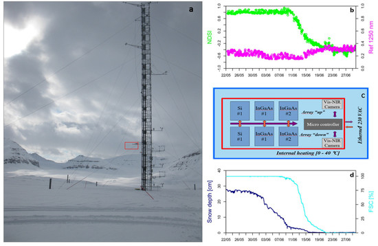
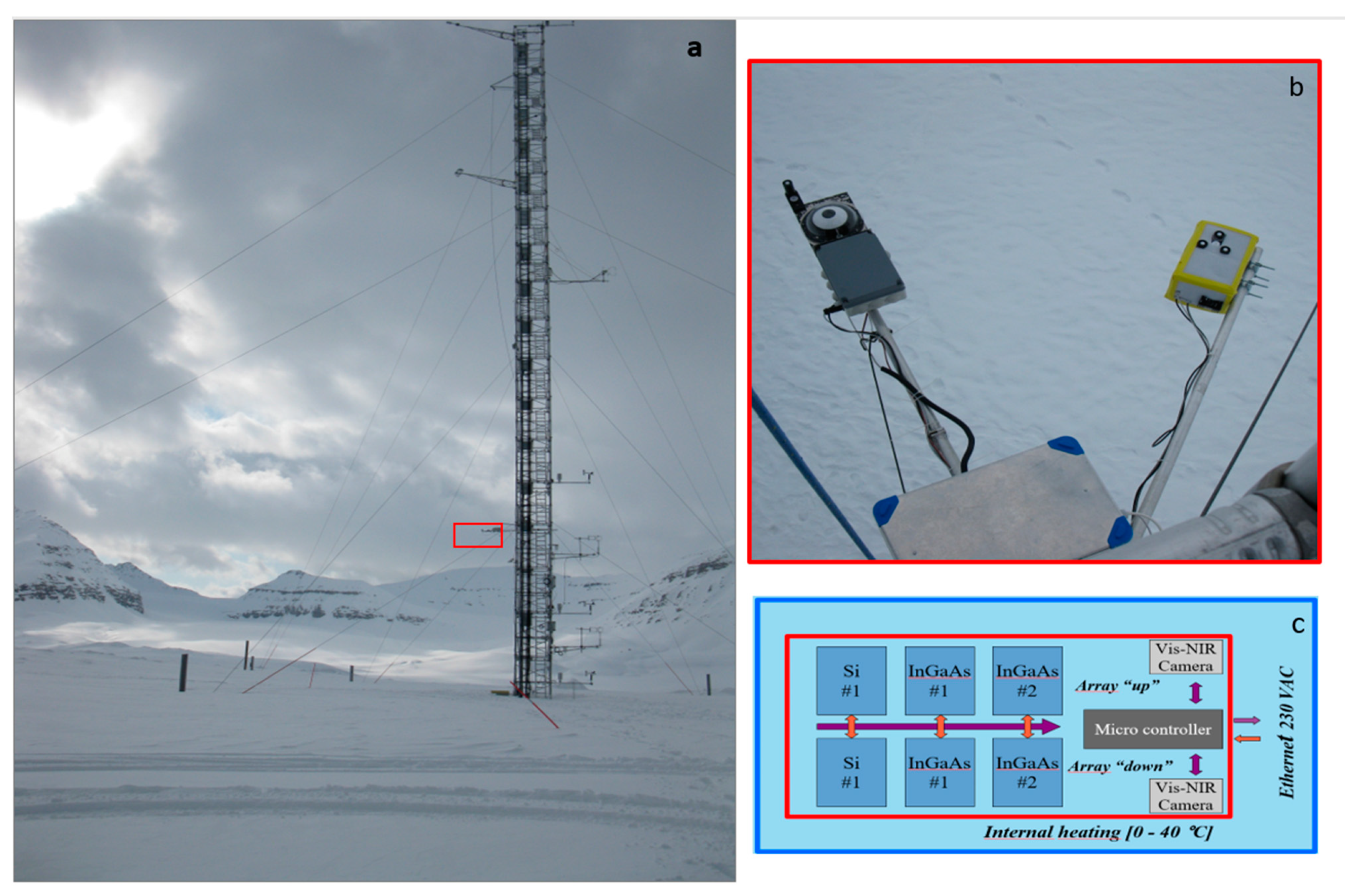
2.1. Continuous Reflectance Monitoring

The continuous monitoring of the spectral albedo was carried out using a custom device, named the continuous reflectance monitor (CReM), with three different narrow bands (10 nm) centered one in the visible (at 550 nm) and two in the short-wave infrared (at 1250 and 1640 nm). The system (Figure 2) is based on commercial parts and it is composed of six different detectors: three sky facing and three oriented towards the surface. The CReM bands 1 and 3 overlap the two bands involved in the NDSI calculation used by the MODIS sensor for Band 4 (545–565 nm) and Band 6 (1628–1652 nm), and by the OLI sensor, onboard of Landsat-8 platform, for Band 3 (525–600 nm) and Band 6 (1560–1660 nm). The CReM band 2 was defined considering the spectral behavior of snow [29] and the attention on that wavelength due to the relationship with the snow microphysics [27]. Band integrations were performed averaging spectral albedo in the selected wavelength ranges. Each sensor is coupled to a teflon (PTFE) diffuser characterized by a geometry such as the Analytical Spectral Device inc. remote cosine receptor. All measurements were synchronous, and the hardware was enclosed in a thermo-stabilized box. The system shown in Figure 2 was implemented combining a data acquisition system programmed through a Python application on a Raspberry Pi microcontroller. The device was installed during the boreal spring nearly 8 m above the ground, as in the experiment described by [10]. The hourly average of the spectral albedo in the three bands was obtained and the standard deviation associated with each cycle provided information about the sky stability, hence, indicating the possibility to perform accurate determination of the spectral albedo.

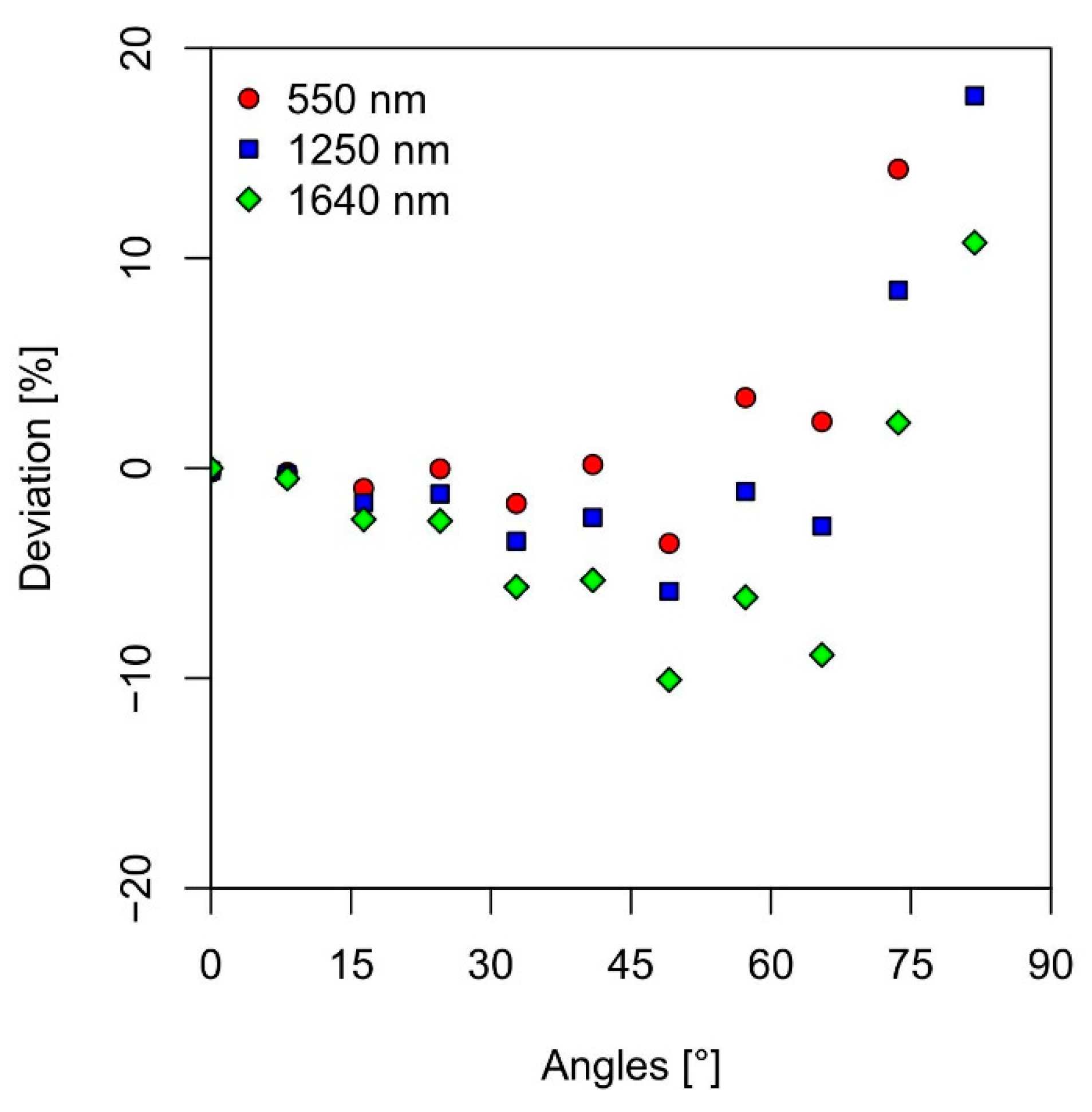
2.1.1. Field of View and Uncertainties

The experimental setup realized for this application, above mentioned, can be defined as bi-hemispherical. The bi-hemispherical reflectance, generally called albedo, is the ratio of the radiant flux reflected from a unit surface area into the whole hemisphere to the incident radiant flux of hemispherical angular extent [14]. This kind of measurement is sensitive to the cosine response of the receiver that could present some deviations, especially at higher sun zenith angles ($\theta$). These deviations, generally largest $\theta$ > 80° [40], imply not negligible uncertainties that can vary at the different wavelengths. Additional anomalies must be considered for the presence of obstacles in the field of view (FOV) [41], such as the tower structure in our case. The two instrumental biases were defined experimentally under laboratory conditions using reference lamps (Figure 3): while the calibration accuracy with the lamp in nadir position was estimated with a maximum error of 2%, the cosine deviation was influenced by solar zenith angle with larger cosine deviations (> 10%) above 70°. In detail, this deviation was lower in the visible range compared to the SWIR. While the Vis deviation was below 5% for $\theta$ < 30° with a maximum deviation at 60° of about 5%, the SWIR deviation was close to 10% at 60°. Considering that the sun zenith angle varied during the survey from 55° to 90°, the dataset was restricted to the sun-facing side of the tower (when the Sun was southward) to reduce the cosine deviation and the contribution of the tower as an obstacle. The spatial representativeness of our experimental setup can be estimated using the approach proposed by [42]. Considering that with an angle of view of 72° more than 90% of the upwelling irradiance is captured, we can assume that the area “seen” by the radiometer is about 3 times the distance from the ground (8 m in our experiment). Finally, we can consider our measurements representative of an area of about a 25 m radius.

2.1.2. Spectral Albedo Estimation

The estimation of the spectral albedo for the selected bands was obtained from the downwelling (${\Phi }_{obs,\lambda }^i$) and upwelling reflected (${\Phi }_{obs,\lambda }^r$) fluxes. For each detector, we considered the specific gain and offset values, controlled at the beginning and at the end of the field campaign. Among correction related to the instrument electronic and acquisition system, to calculate the albedo a simple ratio of the fluxes should be avoided, as the cosine response and the effects of the tower should be considered, also considering the different behavior of the sensor with respect to the direct and diffuse downwelling radiation components. To include such corrections, we assumed the formulation described in [41] and which define the albedo through a corrected ratio of the measured fluxes as follows.

$${\rho }_{\lambda }^{corr}\left({\theta }_i,{\varphi }_i;2\pi \right)=\frac{C_{\lambda }{C}^r{\Phi }_{obs,\lambda }^r}{C_{\lambda }{C}^i(1-d_{\theta }){\Phi }_{obs,\lambda }^i+\frac{d_{\theta }{\Phi }_{obs,\lambda }^i}{1+ϵ\left({\theta }_i\right)}}$$

(4)

This equation includes the average correction factor associated with the cosine response of the detector ($C_{\lambda }$) for diffuse radiation (see Equation (7), [41]), the cosine correction fractional deviation $\epsilon \left({\theta }_i\right)$ associated to the direct component of the flux (Equation (2), [41]), and the correction factor due to the limitation of FOV caused by the tower for the upwelling (Cr) and downwelling fluxes (Ci). Assuming an isotropic surface, the upwelling flux can be considered contributed only by a diffuse component. On the other hand, the downwelling component is contributed by direct and diffuse fluxes that can be discriminated using the direct to global ratio ($d_{\theta }$). As we did not measure the direct and diffuse components of the downwelling spectra irradiance, but the global component only, $d_{\theta }$ was estimated through model calculations for an oceanic aerosol model with optical depth ${\tau }_{550nm}$ of 0.08 and an integrated water vapor content $u_w$ of 0.5 g/cm², and the sun position of each individual albedo acquisition, using the Santa Barbara DISORT Atmospheric Radiative Transfer (SBDART) radiative transfer model [43]. While the diffuse component was corrected similarly to the diffuse component of the upwelling contribution, the direct component was corrected considering the cosine deviation at a specific zenith angle ϵ(θi). Considering the cloudiness of the study area during the survey, particular attention must be addressed to illuminating conditions where the diffuse component is dominant. When cloudiness is higher than 90%, the direct to global incident radiant flux is, in fact, close to zero (dθ ≈ 0). This illumination condition favored the estimation of the so-called white-sky albedo, where angular dependencies are negligible, and corrections are limited to FOV obstructions. Considering that the solid angle occupied by the tower in sky-facing and ground-facing views are similar (Cr ≈ Ci), to estimate the WSA, the previous equation was simplified as follows.

$${\rho }_{\lambda }^{corr}\left(2\pi ;2\pi \right)=\frac{C^r{\Phi }_{obs,\lambda }^r}{C^i{\Phi }_{obs,\lambda }^i}={\rho }_{\lambda }^{obs}\left(2\pi ;2\pi \right)$$

(5)

2.2. Hyperspectral Measurements

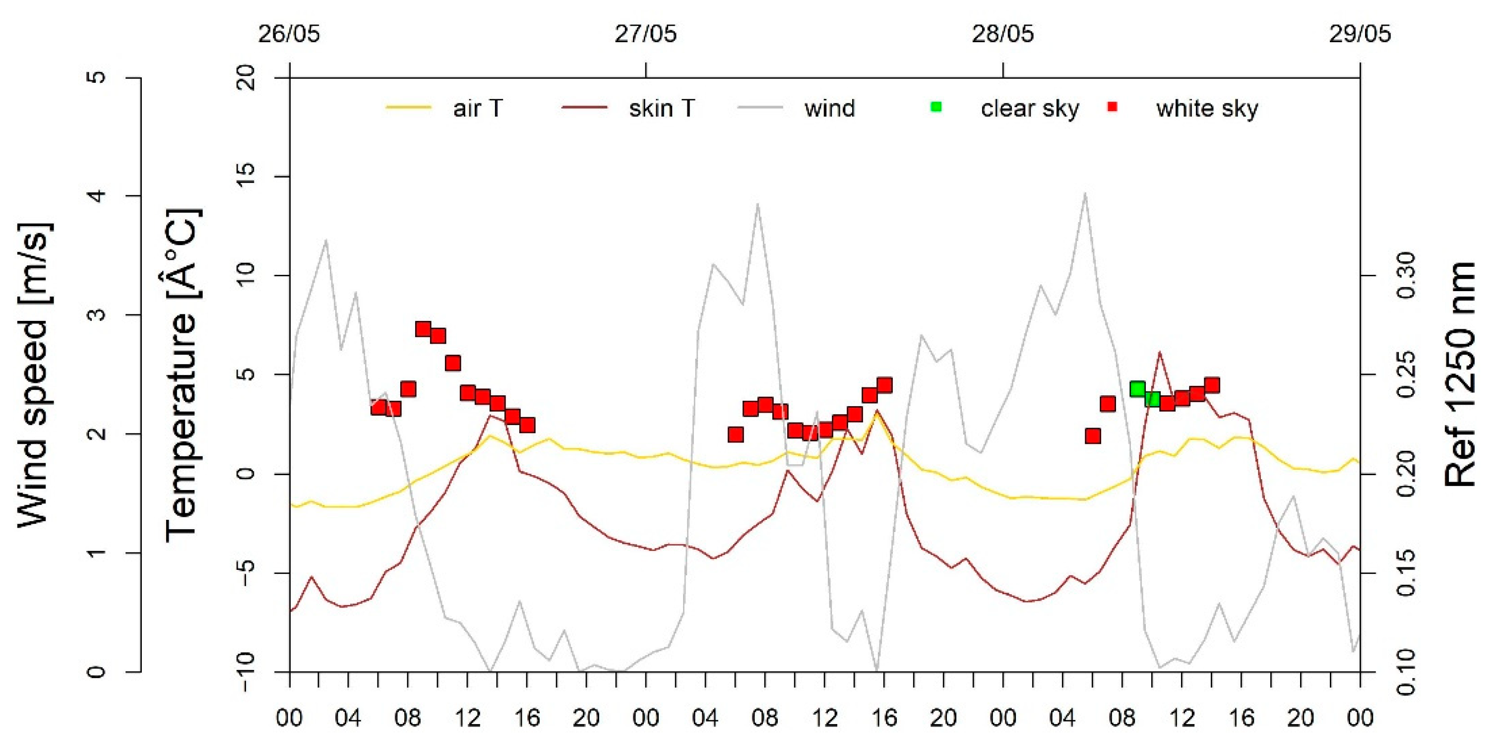
2.2.1. Continuous Observations at the Tower

To collect hyperspectral measurements, an Analytical Spectral Device inc. (ASD) Fieldspec, with a remote cosine receiver (RCR) characterized by a hemispheric field of view, was installed on a tilting device. The collected radiant energy detected by the three spectroradiometers included in the Fieldspec with a wavelength range between 350 and 2500 nm with a maximum spectral resolution of 1 nm. The spectral albedo measurements were acquired using the standard RCR mounted on the tilting system using the procedure described in [10]. An hourly average of spectral albedo was obtained from four measurement cycles performed every 15 min. Dark and optimization operations were executed every hour to estimate gain and spectral offset for each radiometer. Each rotation cycle was composed of a sequence of six downwelling irradiance spectra performed before and after three upwelling measurements, by completing the whole sequence in less than 3 min. All the stored spectra result from the average of ten fast acquisitions. The standard deviation associated with each triplet of spectra provided information on sky stability, hence, indicating the possibility to perform accurate determination of the spectral albedo. The system described in Figure 2b was implemented combining a data acquisition system implemented in LabVIEW (National Instruments), and a tilting system controlled by a Python application on a Raspberry Pi microcontroller. The obtained data were processed considering the methodologies described in Section 2.1.

2.2.2. The Snow Spectral Library

Hyperspectral measurements include also proximal observations that an operator performs using a near-ground setup based on a reference standard for calibrating the instruments [44]. We considered the dataset started to be collected by [45], which is included in the Snow-Ice Spectral Library (SISpec). The absolute spectral reflectance curves in the wavelength range between 350 and 2500 nm were obtained with a Fieldspec portable spectroradiometer (Analytical Spectral Device Inc., Boulder, CO, USA), as a ratio between the radiation reflected from the measured surface and the radiation reflected by a white Spectralon panel. Measurement sites were selected paying particular attention to the different types of snow surface microphysic characteristics (grain type and size) and considering the local weather conditions. All the measurements were collected sun-facing with the optic fiber at about 50 cm above the target and with a nadir orientation. The target identification considered smooth surfaces that could be also recognized and sampled even at the spatial resolution of satellite images (considering a 30 × 30 pixel area of 3 × 3 pixels—approximately 100 × 100 m). Every target was also described from a nivological point of view looking at the shape and size of the grains, density, hardness, and snow temperature. The adopted standard for the description of the snow characteristics was the International classification for seasonal snow on the ground [46].

2.3. Terrestrial Photography

The instrumental setup was completed by a weather-protected fish-eye D-LINK (DCS 6010-L) commercial web-camera, mounted on the same rotating platform. This camera captured photographs of sky and ground conditions every hour (Figure 4), with an increased time resolution (every 15 min) in May and June. The quality check of the available spectra was performed through an algorithm developed with the aim to estimate different ancillary information about the sky cloudiness and the ground conditions. The procedure was based on the analysis of the captured images and the code was developed under the R-project programming environment [47]. Image processing was carried out considering fish-eye distortion and the algorithms for describing cloud and snow covers were the same presented in [10]. The estimation of the cloud-cover index was based on the identification of cloud-free pixels that have been remapped using a weighting mask, which associates the sky-included solid angle with each pixel. A specific mask was used to remove the pixel affected by surrounding mountains and the tower from the image analysis. Then, the true sky-solid angle associated with each pixel has been computed considering the lens distortion, to correctly estimate the cloud cover index. The estimation of clear-sky pixels was based on the combination of the hue and saturation values obtained converting RGB in Hue-Saturation-Value coordinates (HSV). It was assumed that a hue between 180° and 260° (over a full range of 0°–360°) and a saturation greater than 96 (over a full range of 0–255), were associated with blue-sky pixels. The fractional snow cover (FSC) was estimated using the blue-thresholding algorithm proposed by [48].

2.4. The Landsat Imagery

Until the advent of the Sentinel 2 images in 2016, Landsat images were widely used to obtain high-resolution snow cover maps from NDSI images [31,33]. Despite the multiple overpasses of polar-orbiting satellites over the Ny Ålesund area, the high occurrence of clouds affects Landsat images by more than 50% and limits the continuous monitoring of snow cover evolution [36]. The Landsat 8 catalog and the LC08_L1TP product includes the study area from May to July 2015 about 50 scenes, but for the above-mentioned reasons, only 6 are free of clouds in the area on which the CReM is located. These 6 images were radiometrically calibrated and atmospherically corrected with the ENVI software [49,50]. A buffer region of 3×3 pixels around the study site was used to extract the average reflectance values. The spatial resolution at the ground of the Landsat images is 30 m per pixel.

2.5. Additional Data

The climate change tower facility hosts different sensors (temperature, relative humidity, pressure, wind direction, and speed) at 0 (skin), 2, 5, 10, and 30 m above the snow-free ground [51]. A four-component net radiometer CNR-1 (Kipp and Zonen) collecting the broadband shortwave and longwave components of the surface radiation balance is installed on the top of the tower at a 32 m level. The shortwave components are measured by means of two CM3 pyranometers which cover the spectral range 305–2800 nm with a field of view of 180° and an uncertainty of 5% up to 80° solar zenith angle [51]. They are stored as 1-min averages of 1-Hz acquisitions.

3. Results

The analysis of the available image pairs (facing to the sky and to the ground) acquired by the tilting system during the survey covered 1730 h and included about 400 situations when the alignment of the rotating system confirmed a near-optimal orientation towards either the sky or the ground as well as a sun position that limited the tower interference. We filtered the dataset, in fact, considering only the sun azimuth from 90° E to 270° E in order to reduce the biases produced by the tower structure. The sun elevation above 15° represented additional criteria for filtering the dataset in order to limit the uncertainties associated with the cosine deviation produced by the selected diffusers.

The cloud cover index retrieved by the selected sky imagery discriminated between different illumination conditions. A threshold of 90% of cloud cover index defined of the diffuse light condition and a cloud cover index lower than 10% identified of cloud-free sky where direct irradiation is dominant. With this assumption approximately 49% of images were flagged as pertaining to diffuse conditions, hence to albedo taken in white-sky conditions (WSA), while only 9% of the images identified as clear-sky and associated to albedo measurements evaluated in clear-sky conditions (CSA). The comparison between the estimated WSA and CSA values, for the three selected bands, by the CReM device and the ASD-based system demonstrated a good agreement between the two different approaches (Figure 5). The comparison based on about 400 observations with 25% of CSA and 75% WSA situations. The resulting RMSEs were respectively 0.024, 0.023, and 0.022 for the three bands.

The results concerning both WSA and CSA situations presented in Figure 6 showed that the observing period presented typical features of the melting season with reflectance, in the different wavelength ranges, in agreement with the SISpec library from the beginning of the campaign (21 May) to 9 June. From 9 June to 15 June, it was possible to observe a rapid decrease in the visible band (from more than 0.8 to below 0.2), coupled with a significant increase in the SWIR bands, respectively from 0.3 and 0.15 to 0.4 and 0.35. While the reduction of reflectance at 550 nm and the increase of reflectance at 1640 nm were significant, the ramp from May to July detected at 1250 nm was smoother. It is important to notice that remotely sensed observations were limited to 6 acquisitions, considering the Landsat-8 platform, and that algorithms aimed at estimating the surface reflectance require additional effort on retrieving values compliant with in-situ measurements.

4. Discussion

The evolution of the snow cover during a melting season can be described through two optical features: the SWIR reflectance and relationship between the visible and the SWIR range (Figure 7). While the SWIR analysis could describe the evolution of the snow surface in terms of macro and micro physics, the second feature can discriminate the presence or not of snow cover. The first feature was approached considering the albedo at 1250 nm, which varied from above 0.25 on May to below 0.2 on 9 June.

This general trend was coupled with short-time fluctuations that could be associated with short-time variations of meteo-climatic conditions (air temperature, relative humidity, wind speed). This association could be significant especially when the air-ground temperature gradient favors the formation of surface hoars, but further technological improvements are required for differentiating such fluctuations from the measurement uncertainties. The melting conditions favor evaporation due to the water vapor gradient affecting the snow profile. If abrupt temperature decreases occur, crystallization associated with sublimation implies the formation of hoars or faceted crystals at different depths of the profile. Figure 8 evidence such behavior on a 24-h time window. The increase of 1250 nm reflectance is related to the SSA increment [27] when sublimation produced small-sized crystals [52]. Looking at wind calm conditions between 26 May and 29 May, it was possible to evidence a complex dynamic system that needs more effort for complete comprehension.

The importance of the evolution concerning the SWIR albedo can be interpreted by examining the relationship between these spectral features and the specific surface area of the snow cover, the surface roughness, and the presence of impurities in snow. Concerning SSA, we are not ready to define a quantitative SSA calibration for our method, but this association was already defined for bidirectional light conditions [27] and by models [5]. From a general point of view, the evolution of this spectral feature could highlight high and low SSA conditions of the snowed surface that were strictly related to precipitation events and high wind-speed conditions. The SSA, in fact, can be higher only when fresh snow, characterized by dendritic grains, occurs or when wind ablation produces surface-grain fragmentation. On the opposite, SSA could be lower when snow metamorphism occurs, thus grains increase in dimension and change in shape to round and compact grain-types.

The alteration of albedo associated with the surface roughness could be therefore an additional issue [40]. This contribution to the determination of the true albedo is limited in our study by the height of the sensor [53], by the restriction to diffuse light conditions (measuring WSA), and by the roughness features of the study site [18,52]. Some authors [18] presented a roughness bias in the order of 0.02–0.04 for the visible range and there are no estimations in literature for the SWIR domain. Finally, the presence of impurities in the shallow snow layer is an additional critical issue, which requires specific investigations that are not included in our objectives now. Impurities, black and brown carbon, can impact significantly spectral albedo, especially in the visible wavelength range [54]. The contribution of such components in the SWIR range is limited considering the amount of soot present in the Svalbard site. The availability of the new dataset will surely improve the modeling capacity, but it is feasible to assume a limited contribution of impurities at 1600 nm. Further investigations will be necessary in order to interpret all these phenomena and specific analysis must be addressed for estimating the different contributions to the spectral albedo.

The most common spectral feature used in remote sensing for the characterization of snowed surfaces is the NDSI, which is calculated coupling visible and shortwave infrared bands of the available sensor. The CReM system is characterized by an NDSI calculated considering the 550 nm and the 1640 nm bands. The evolution of the NDSI was strictly related to the snow aging in the first period of the melting season (up to 9 June), when the snow depth reduction was more consistent. This transition was characterized by NDSI values above 0.6 with temperatures generally below 0 °C and short fluctuations above 0 °C. From 9 June to 15 June the air temperature started to rise rapidly above 0 °C and the NDSI reached a plateau level of −0.5 °C from 15 June to the end of July. The snow depth in this second period continued to decrease and the NDSI plateau was discontinued just in occurrence of precipitation events. Considering the NDSI estimated by CReM for snowed surfaces between 20 May and 10 June, we observed values of about 0.81 that were such as those detected by Landsat, processed as bottom-of-atmosphere reflectance (NDSI_BOA ~ 0.87).

The relationship between the observed FSC and NDSI outlined a highly correlated evolution characterized by r² 0.98. The relation was good when FSC values ranged between 5% to 95%. A soft reduction of those variables was triggered by the snow depth at 10 cm. After 8 days the FSC drastically decreased to 25% and NDSI was 0. This melting phase reached a snow depth almost negligible on 15 June. Considering the definition of an NDSI threshold for discriminating between snow-covered surfaces and bare soil areas [38], a site-specific threshold is defined with NDSI = 0.2, when the FSC is above 50%. This value is lower than the reference threshold of 0.4 [13], but it is well demonstrated that high-resolved observations could identify this kind of value [55].

This phase was characterized by snow melting of about 2 cm/day associated with a rapid increase of the skin temperature T_skin (from −5 to approximately 0 °C) over this time extent. The last period differed substantially from the previous two, thus the skin temperature started to rise to 5 °C at the end of the period. Summarizing the differences, the first period showed a near-melting condition (T_air ~ 0 °C) that facilitates water-ice transformation associated with temperature fluctuations. The second period presented an intermediate-melting condition (T_air > 0 °C) and the last one was characterized by the conclusion of the melting behavior (T_air >> 0 °C).

5. Conclusions

This work presented the field activity carried out in Ny Ålesund during the 2015 spring/summer period at the CNR Climate Change Tower. The continuous monitoring of snow surfaces in polar regions was approached by installing a narrow band system (CReM) in addition to a full range spectroradiometer. We explored the opportunity to have a routinely operating system instead of complex hyperspectral devices aimed at analyzing the snow spectral behavior during the melting season. The proposed system supports the quality check of the acquired data with sky and ground images useful in assessing the different illumination and surface conditions. The first results permitted us to assess the feasibility of continuously monitoring the spectral evolution of snowed surfaces without any man intervention. The developed device supported the qualitative characterization of spectral variations during the melting period. It was possible to estimate spectral indexes, such as NDSI and SWIR albedo and we have found interesting links between both features and air/ground temperatures, wind-speed, and precipitations. Different melting phases were detected, and different processes were associated with the observed spectral variations. This study represents a starting point for having a continuous ground-truth of the snow optical behavior. The extension of this kind of observation to the SWIR wavelength domain offers different opportunities for associating snow metamorphism to spectral variations and on validating remotely sensed data. Further technological developments and a less disturbed experimental setup are required in order to identify relevant correlations with meteorological parameters.

References

1. Callaghan, T.V.; Johansson, M.; Brown, R.D.; Groisman, P.Y.; Labba, N.; Radionov, V.; Barry, R.G.; Bulygina, O.N.; Essery, R.L.H.; Frolov, D.M.; et al. The Changing Face of Arctic Snow Cover: A Synthesis of Observed and Projected Changes. Ambio 2011, 40, 17–31. [Google Scholar] [CrossRef] [Green Version]
2. Dozier, J.; Painter, T.H.; Rittger, K.; Frew, J.E. Time-space continuity of daily maps of fractional snow cover and albedo from MODIS. Adv. Water Resour. 2008, 31, 1515–1526. [Google Scholar] [CrossRef]
3. Eastman, R.; Warren, S.G. Arctic Cloud Changes from Surface and Satellite Observations. J. Clim. 2010, 23, 4233–4242. [Google Scholar] [CrossRef] [Green Version]
4. Nolin, A.W. Recent advances in remote sensing of seasonal snow. J. Glaciol. 2010, 56, 1141–1150. [Google Scholar] [CrossRef] [Green Version]
5. Gallet, J.C.; Domine, F.; Zender, C.S.; Picard, G. Measurement of the specific surface area of snow using infrared reflectance in an integrating sphere at 1310 and 1550 nm. Cryosphere 2009, 3, 167–182. [Google Scholar] [CrossRef] [Green Version]
6. Painter, T.H.; Molotch, N.P.; Cassidy, M.; Flanner, M.; Steffen, K. Contact spectroscopy for determination of stratigraphy of snow optical grain size. J. Glaciol. 2007, 53, 121–127. [Google Scholar] [CrossRef] [Green Version]
7. Bourgeois, C.S.; Calanca, P.; Ohmura, A. A field study of the hemispherical directional reflectance factor and spectral albedo of dry snow. J. Geophys. Res. 2006, 111, D20108. [Google Scholar] [CrossRef] [Green Version]
8. Marks, A.; Fragiacomo, C.; MacArthur, A.; Zibordi, G.; Fox, N.; King, M.D. Characterisation of the HDRF (as a proxy for BRDF) of snow surfaces at Dome C, Antarctica, for the inter-calibration and inter-comparison of satellite optical data. Remote Sens. Environ. 2015, 158, 407–416. [Google Scholar] [CrossRef]
9. Picard, G.; Arnaud, L.; Domine, F.; Fily, M. Determining snow specific surface area from near-infrared reflectance measurements: Numerical study of the influence of grain shape. Cold Reg. Sci. Technol. 2009, 56, 10–17. [Google Scholar] [CrossRef]
10. Salzano, R.; Lanconelli, C.; Salvatori, R.; Esposito, G.; Vitale, V. Continuous monitoring of spectral reflectance of snowed surfaces in Ny-Ålesund. Rend Fis Acc Lincei 2016, 27, 137–149. [Google Scholar] [CrossRef]
11. Painter, T.H.; Dozier, J.; Roberts, D.A.; Davis, R.E.; Green, R.O. Retrieval of subpixel snow-covered area and grain size from imaging spectrometer data. Remote Sens. Environ. 2003, 85, 64–77. [Google Scholar] [CrossRef] [Green Version]
12. Tedesco, M.; Kokhanovsky, A.A. The semi-analytical snow retrieval algorithm and its application to MODIS data. Remote Sens. Environ. 2007, 111, 228–241. [Google Scholar] [CrossRef]
13. Dietz, A.J.; Kuenze, C.R.; Gessner, U.; Dech, S. Remote sensing of snow—A review of available methods. Int. J. Remote Sens. 2011, 33, 4094–4134. [Google Scholar] [CrossRef]
14. Schaepman-Strub, G.; Schaepman, M.E.; Painter, T.H.; Dangel, S.; Martonchik, J.V. Reflectance quantities in optical remote sensing—definitions and case studies. Remote Sens. Environ. 2006, 103, 27–42. [Google Scholar] [CrossRef]
15. Lewis, P.; Barnsley, M.J. Influence of the sky radiance distribution on various formulations of the earth surface albedo. In Proceedings of the Conference Physics Measures, Signals and Remote Sensing, Val d’Isere, France, 17–21 January 1994; pp. 707–715. [Google Scholar]
16. Liu, J.; Schaaf, C.; Strahler, A.; Jiao, Z.; Shuai, Y.; Zhang, Q.; Roman, M.; Augustine, J.A.; Dutton, E.G. Validation of Moderate Resolution Imaging Spectroradiometer (MODIS) albedo retrieval algorithm: Dependence of albedo on solar zenith angle. J. Geophys. Res. 2009, 114, D01106. [Google Scholar] [CrossRef]
17. Painter, T.H.; Roberts, D.A.; Green, R.O.; Dozier, J. The Effect of Grain Size on Spectral Mixture Analysis of Snow-Covered Area from AVIRIS Data. Remote Sens. Environ. 1998, 65, 20–332. [Google Scholar] [CrossRef]
18. Warren, S.G.; Brandt, R.E.; O’Rawe Hinton, P. Effect of surface roughness on bidirectional reflectance of Antarctic snow. J. Geophys. Res. 1998, 103, 25789–25807. [Google Scholar] [CrossRef]
19. Pedersen, C.A.; Gallet, J.C.; Ström, J.; Gerland, S.; Hudson, S.R.; Forsström, S.; Isaksson, E.; Berntsen, T.K. In situ observations of black carbon in snow and the corresponding spectral surface albedo reduction. J. Geophys. Res. Atmos. 2015, 120, 1476–1489. [Google Scholar] [CrossRef]
20. Warren, S.G. Can black carbon in snow be detected by remote sensing? J. Geophys. Res. Atmos. 2013, 118, 779–786. [Google Scholar] [CrossRef] [Green Version]
21. Doherty, S.J.; Warren, S.G.; Grenfell, T.C.; Clarke, A.D.; Brandt, R.E. Light-absorbing impurities in Arctic snow. Atmos. Chem. Phys. 2010, 10, 11647–11680. [Google Scholar] [CrossRef] [Green Version]
22. Forsstrom, S.; Strom, J.; Pedersen, C.A.; Isaksson, E.; Gerland, S. Elemental carbon distribution in Svalbard snow. J. Geophys. Res. 2009, 114, D19112. [Google Scholar] [CrossRef]
23. Qian, Y.; Yasunari, T.J.; Doherty, S.J.; Flanner, M.G.; Lau, W.K.M.; Ming, J.; Wang, H.; Wang, M.; Warren, S.G.; Zhang, R. Light-absorbing Particles in Snow and Ice: Measurement and Modeling of Climatic and Hydrological impact. Adv. Atmos. Sci. 2015, 32, 64–91. [Google Scholar] [CrossRef]
24. Doherty, S.J.; Dang, C.; Hegg, D.A.; Zhang, R.; Warren, S.G. Black carbon and other light-absorbing particles in snow of central North America. J. Geophys. Res. Atmos. 2014, 119, 12807–12831. [Google Scholar] [CrossRef]
25. Huang, J.; Fu, Q.; Zhang, W.; Wang, X.; Zhang, R.; Ye, H.; Warren, S.G. Dust and Black Carbon in Seasonal Snow Across Northern China. Bull. Am. Meteorol. Soc. 2011, 92, 175–181. [Google Scholar] [CrossRef] [Green Version]
26. Negi, H.S.; Kokhanovsky, A.A. Retrieval of snow grain size and albedo of western Himalayan snow cover using satellite data. Cryosphere 2011, 5, 831–847. [Google Scholar] [CrossRef] [Green Version]
27. Dominé, F.; Salvatori, R.; Legagneux, L.; Salzano, R.; Fily, M.; Casacchia, R. Correlation between the specific surface area and the short wave infrared (SWIR) reflectance of snow. Cold Reg. Sci. Technol. 2006, 46, 60–68. [Google Scholar] [CrossRef]
28. Warren, S.G. Optical properties of Snow. Rev. Geophys. Space Phys. 1982, 20, 67–89. [Google Scholar] [CrossRef]
29. Warren, S.G.; Wiscombe, W.J. A model for the spectral albedo of snow, II, Snow containing atmospheric aerosols. J. Atmos. Sci. 1980, 37, 2734–2745. [Google Scholar] [CrossRef]
30. Wiscombe, W.J.; Warren, S.G. A model for the spectral albedo of snow, I, Pure snow. J. Atmos. Sci. 1980, 37, 2712–2733. [Google Scholar] [CrossRef] [Green Version]
31. Dozier, J. Spectral signature of alpine snow cover from the Landsat thematic mapper. Remote Sens. Environ. 1989, 28, 9–22. [Google Scholar] [CrossRef]
32. Fily, M.; Bourdelles, B.; Dedieu, J.P.; Sergent, C. Comparison of in situ and Landsat Thematic Mapper derived snow grain characteristics in the Alps. Remote Sens. Environ. 1997, 59, 452–460. [Google Scholar] [CrossRef]
33. Rees, W.G. Remote Sensing of Snow and Ice; CRC press—Taylor & Francis Ed: Boca Raton, FL, USA, 2006. [Google Scholar]
34. Hall, D.K.; Riggs, G.A.; Salomonson, V.V.; DiGirolamo, N.E.; Bayr, K.J. Modis snow-cover products. Remote Sens. Environ. 2002, 83, 181–194. [Google Scholar] [CrossRef] [Green Version]
35. Poggio, L.; Gimona, A. Sequence-based mapping approach to spatio-temporal snow patterns from MODIS time-series applied to Scotland. Int. J. Appl. Earth Obs. Geoinf. 2015, 34, 122–135. [Google Scholar] [CrossRef]
36. Gascoin, S.; Grizonnet, M.; Bouchet, M.; Salgues, G.; Hagolle, O. Theia Snow collection: High-resolution operational snow cover maps from Sentinel-2 and Landsat-8 data. Earth Syst. Sci. 2019, 11, 493–514. [Google Scholar] [CrossRef] [Green Version]
37. Yin, D.; Cao, X.; Chen, X.; Shao, Y.; Chen, J. Comparison of automatic thresholding methods for snow-cover mapping using Landsat TM imagery. Int. J. Remote Sens. 2013, 34, 6529–6538. [Google Scholar] [CrossRef]
38. Solomonson, V.V.; Appel, I. Estimating fractional snow cover from MODIS using the normalized difference snow index. Remote Sens. Environ. 2004, 89, 351–360. [Google Scholar] [CrossRef]
39. Vogel, S.W. Usage of high-resolution Landsat 7 band 8 for single snow-cover classification. Ann. Glaciol. 2002, 34, 53–57. [Google Scholar] [CrossRef] [Green Version]
40. Pirazzini, R. Surface albedo measurements over Antarctic sites in summer. J. Geophys. Res. 2004, 109, D20118. [Google Scholar] [CrossRef]
41. Carmagnola, C.M.; Domine, F.; Dumont, M.; Wright, P.; Strellis, B.; Bergin, M.; Dibb, J.; Picard, G.; Libois, Q.; Arnaud, L.; et al. Snow spectral albedo at Summit, Greenland: Measurements and numerical simulations based on physical and chemical properties of the snowpack. Cryosphere 2013, 7, 1139–1160. [Google Scholar] [CrossRef] [Green Version]
42. Kassianov, E.; Barnard, J.; Flynn, C.; Riihimaki, L.; Michalsky, J.; Hodges, G. Areal-Averaged Spectral Surface Albedo from Ground-Based Transmission Data Alone: Toward an Operational Retrieval. Atmosphere 2014, 5, 597–621. [Google Scholar] [CrossRef] [Green Version]
43. Ricchiazzi, P.; Yang, S.; Gautier, C.; Sowle, D. SBDART: A research and teaching software tool for plane-parallel radiative transfer in the Earth’s atmosphere. Bull. Am. Meteorol. Soc. 1998, 79, 2101–2114. [Google Scholar] [CrossRef] [Green Version]
44. Casacchia, R.; Lauta, F.; Salvatori, R.; Cagnati, A.; Valt, M.; Orbek, J.B. Radiometric investigation on different snow covers in Svalbard. Polar Res. 2001, 20, 13–22. [Google Scholar] [CrossRef] [Green Version]
45. Salvatori, R.; Casacchia, R.; Ghergo, S.; Firmani, M.; Cagnati, A.; Valt, M.; Lauta, F.; Di Mambro, V. SISpec—Snow Ice Spectral archive. AIT Acad. Inf. Technol. 2000, 17, 3–8. [Google Scholar]
46. Fierz, C.; Armstrong, R.L.; Durand, Y.; Etchevers, P.; Greene, E.; McClung, D.M.; Nishimura, K.; Satyawali, P.K.; Sokratov, S.A. The International Classification for Seasonal Snow on the Ground. In Technical Documents in Hydrology 83, IACS Contribution N°1; UNESCO-IHP: Paris, France, 2009. [Google Scholar]
47. A Language and Environment for Statistical Computing. Available online: http://www.R-project.org/ (accessed on 30 December 2020).
48. Salvatori, R.; Plini, P.; Giusto, M.; Valt, M.; Salzano, R.; Montagnoli, M.; Cagnati, A.; Crepaz, G.; Sigismondi, G. Snow cover monitoring with images from digital camera systems. Int. J. Remote Sens. 2011, 43, 137–145. [Google Scholar] [CrossRef]
49. Isaacs, R.G.; Wang, W.C.; Worsham, R.D.; Goldenberg, S. Multiple Scattering LOWTRAN and FASCODE Models. Appl. Opt. 1987, 26, 1272–1281. [Google Scholar] [CrossRef] [PubMed]
50. Stamnes, K.; Tsay, S.C.; Wiscombe, W.; Jayaweera, K. Numerically Stable Algorithm for Discrete-Ordinate-Method Radiative Transfer in Multiple Scattering and Emitting Layered Media. Appl. Opt. 1988, 27, 2502–2509. [Google Scholar] [CrossRef]
51. Mazzola, M.; Viola, A.; Lanconelli, C.; Vitale, V. Atmospheric observations at the Amundsen-Nobile Climate Change Tower in Ny-Ålesund, Svalbard. Rend Fis Acc Lincei 2016, 27, 7–18. [Google Scholar] [CrossRef]
52. Valt, M.; Salvatori, R. Snowpack characteristics of Brøggerhalvøya, — Svalbard Islands. Rend Fis Acc Lincei 2016, 27, 129–136. [Google Scholar] [CrossRef]
53. Lhermitte, S.; Abermann, J.; Kinnardet, C. Albedo over rough snow and ice surfaces. Cryosphere 2014, 8, 1069–1086. [Google Scholar] [CrossRef] [Green Version]
54. Kokhanovsky, A.A. Spectral reflectance of solar light from dirty snow: A simple theoretical model and its validation. Cryosphere 2013, 7, 1325–1331. [Google Scholar] [CrossRef] [Green Version]
55. Härer, S.; Bernhardt, M.; Siebers, M.; Schulz, K. On the need for a time- and location-dependent estimation of the NDSI threshold value for reducing existing uncertainties in snow cover maps at different scales. Cryosphere 2018, 12, 1629–1642. [Google Scholar] [CrossRef]
Figure 1. Location map of the study site: Ny Ålesund (Svalbard, Norway).
Geosciences 11 00112 g001
Figure 2. A view of the Amundsen-Nobile Climate Change Tower (a) with instruments installed at different levels; our system is highlighted by the red rectangle (8 m). The deployment of the CReM and ASD-based systems (b). The components of the CReM device (c).
Geosciences 11 00112 g002
Figure 3. The cosine deviation of reflectance for the selected diffuser.
Geosciences 11 00112 g003
Figure 4. Examples of camera views facing to the sky (a) (6 July 2015 14:30UTC) and to the ground (14 June 2015 14:00UTC). The fractional snow cover of picture (b) was estimated as 35%.
Geosciences 11 00112 g004
Figure 5. Comparison between reflectance measurements at different wavelengths provided by the Fieldspec ASD system at the tower and the CReM device. The red line represents a 1:1 relationship.
Geosciences 11 00112 g005
Figure 6. CReM reflectance values (red/green) for the three selected bands versus the available data acquired by the Landsat-8 platform (blue). The grey areas represent the statistical values obtained by the SISpec library and reported in terms of 10th–90th percentiles (grey) and the median reflectance (dark grey).
Geosciences 11 00112 g006
Figure 7. Comparison between the optical behavior of snow and the meteo-climatological information about the melting season 2015.
Geosciences 11 00112 g007
Figure 8. Examples of short-term variations of reflectance at 1250 nm in May 2015.
Geosciences 11 00112 g008
Publisher’s Note: MDPI stays neutral with regard to jurisdictional claims in published maps and institutional affiliations.