Stiffness and Strength of Stabilized Organic Soils—Part II/II: Parametric Analysis and Modeling with Machine Learning

Abstract

Predicting the range of achievable strength and stiffness from stabilized soil mixtures is critical for engineering design and construction, especially for organic soils, which are often considered “unsuitable” due to their high compressibility and the lack of knowledge about their mechanical behavior after stabilization. This study investigates the mechanical behavior of stabilized organic soils using machine learning (ML) methods. ML algorithms were developed and trained using a database from a comprehensive experimental study (see Part I), including more than one thousand unconfined compression tests on organic clay samples stabilized by wet soil mixing (WSM) technique. Three different ML methods were adopted and compared, including two artificial neural networks (ANN) and a linear regression method. ANN models proved reliable in the prediction of the stiffness and strength of stabilized organic soils, significantly outperforming linear regression models. Binder type, mixing ratio, soil organic and water content, sample size, aging, temperature, relative humidity, and carbonation were the control variables (input parameters) incorporated into the ML models. The impacts of these factors were evaluated through rigorous ANN-based parametric analyses. Additionally, the nonlinear relations of stiffness and strength with these parameters were developed, and their optimum ranges were identified through the ANN models. Overall, the robust ML approach presented in this paper can significantly improve the mixture design for organic soil stabilization and minimize the experimental cost for implementing WSM in engineering projects.

1. Introduction

Organic soils are widely accessible yet often avoided in construction projects due to their high compressibility and lack of knowledge about proper stabilization techniques and the behavior of stabilized organic soils. Extensive studies have investigated the mechanical behavior of stabilized mineral soils. However, only a limited number of studies have addressed stabilized organic soils’ behavior, leaving a knowledge gap in this field [1,2,3,4,5,6,7,8,9,10,11,12,13,14,15,16,17].

One of the most commonly used methods to improve soil stiffness and strength is deep soil mixing (DSM). DSM is a cost-effective method for organic soil improvement using binders; however, as an evolving field, it still requires further knowledge and understanding through experimental and numerical investigations [18].

Mechanical properties (stiffness and strength) of stabilized soils are related to several soil and binder mixture properties and experimental factors (control variables). Investigating the effects of these variables and their interactions becomes increasingly complicated as the number of variables increases. For such a high-dimensional system, machine learning (ML) can provide a powerful tool to capture nonlinearities and the complex relations between the control variables and the target parameter.

This study introduces a novel ML approach to predict the stiffness (unconfined tangent modulus at 50% of the maximum stress, E) and unconfined compression strength (UCS) of stabilized organic soils. The predictive models were developed based on a database of UCS tests on organic clay samples stabilized using the wet soil mixing (WSM) method (see Part I [19,20]). Effects of various control variables on the mechanical behavior of stabilized organic soils were investigated using ML methods. The control variables included organic content (OC), water content (w), the ratio of binder (RB), the quantity of binder (QB), grout to soil ratio (G/S), water to binder ratio (W/B), sample size (diameter to height ratio, D/H), aging (time, t), temperature (T), relative humidity (RH), and carbonation (CO₂).

Two prominent ANN algorithms, radial basis function (RBF) and multilayer perceptron (MLP), and the multiple linear regression (MLR) method were implemented, and their performance was analyzed and compared. Additionally, the stepwise parameter selection method was implemented to identify the most influential control variables, reduce the dimensionality, and optimize the ANN models’ performance. Moreover, an ANN-based sensitivity analysis method was adopted to investigate each control variable’s impact and identify their optimum range for maximizing the strength and stiffness of stabilized organic soils.

2. Background

ANNs have been widely used in various geotechnical applications [21], such as in prediction of pile capacity [22,23,24,25,26,27,28,29,30], constitutive modeling of soil [31,32,33,34,35,36,37], site characterization [38,39], earth-retaining structures [40], settlement of foundations [41,42], prediction of unknown foundations [43], slope stability [44,45], design of tunnels and underground openings [46,47], liquefaction [48,49,50,51,52], soil permeability and hydraulic conductivity [53], soil compaction [54,55], and soil classification [56,57].

Some studies have applied ANNs to model the stiffness and strength of stabilized soils and other cement-based products. Tinoco et al. [58] applied ML methods including ANNs, support vector machines (SVM), and MLR to predict the UCS based on a compiled database (444 records) from multiple experimental studies on a variety of soil-cement mixtures. They reported both ANN and SVM to predict the UCS with high accuracy. They found water to cement ratio, cement content, organic content, and the mixture’s age to be the most influential parameters. Molaabasi et al. [59] applied the group method of data handling (GMDH)-type ANNs to predict the stress–strain behavior of zeolite-cemented sand based on results of 216 UCS tests, showing GMDH can be a reliable tool for capturing the influence of various parameters on the behavior of stabilized sand mixtures. Suman et al. [60] developed predictive models for the UCS of cement-stabilized soils using functional networks and multivariate adaptive regression splines based on a literature database, reporting these AI techniques’ generalization ability to be better than ANNs. They found the most influential input parameters to be moisture content and gravel content, among others (Atterberg limits, sand and cement content). Cement content was not as significant due to the generally low cement content of samples in this database. Wang and Al-Tabbaa [61] used Bayesian predictive neural network models to predict the UCS values of cement-stabilized soils (inorganic) as a function of selected soil mix variables, such as grain size distribution, water content, cement content, and curing time. Shrestha and Al-Tabbaa [62] established trends using ANNs between UCS as a function of selected soil mix variables such as initial soil water content and binder dosage. Stegemann and Buenfeld [63,64,65] performed a series of ANN analyses to predict the UCS of cement-solidified wastes and developed nonlinear correlations between the UCS and waste quantities. They also evaluated the effects of contaminants and hydraulic binders. Narendra et al. [66] proposed a generic mathematical model using ANNs based on MLP, RBF, and genetic programming (GP) developed based on laboratory tests conducted on stabilized inorganic clays with varying water contents, cement contents, and curing periods. MLP was shown to have the highest prediction accuracy, followed by GP, RBF, and other empirical models. Das et al. [67] applied MLPs with Levenberg–Marquardt optimization, Bayesian regularization, and differential evolution algorithms for predicting the UCS and maximum dry density of cement-stabilized soils, incorporating Atterberg limits, gradation, and cement and water content as input parameters. Mozumder and Laskar [68] applied MLP models with Bayesian regularization algorithm for predicting the UCS for geopolymer stabilized clays with blast furnace slag and fly ash, reporting ANNs to outperform MLR models.

3. Modeling

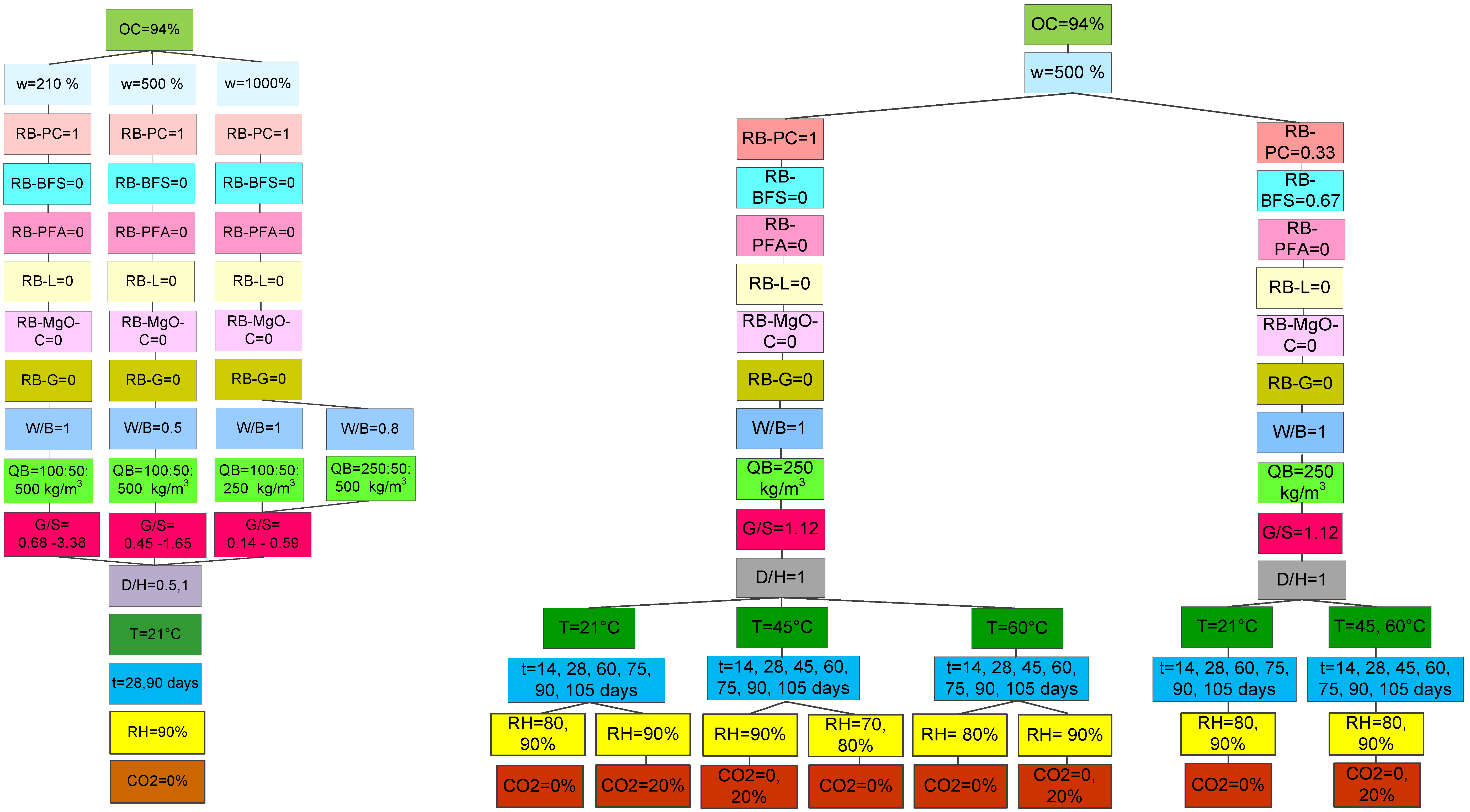
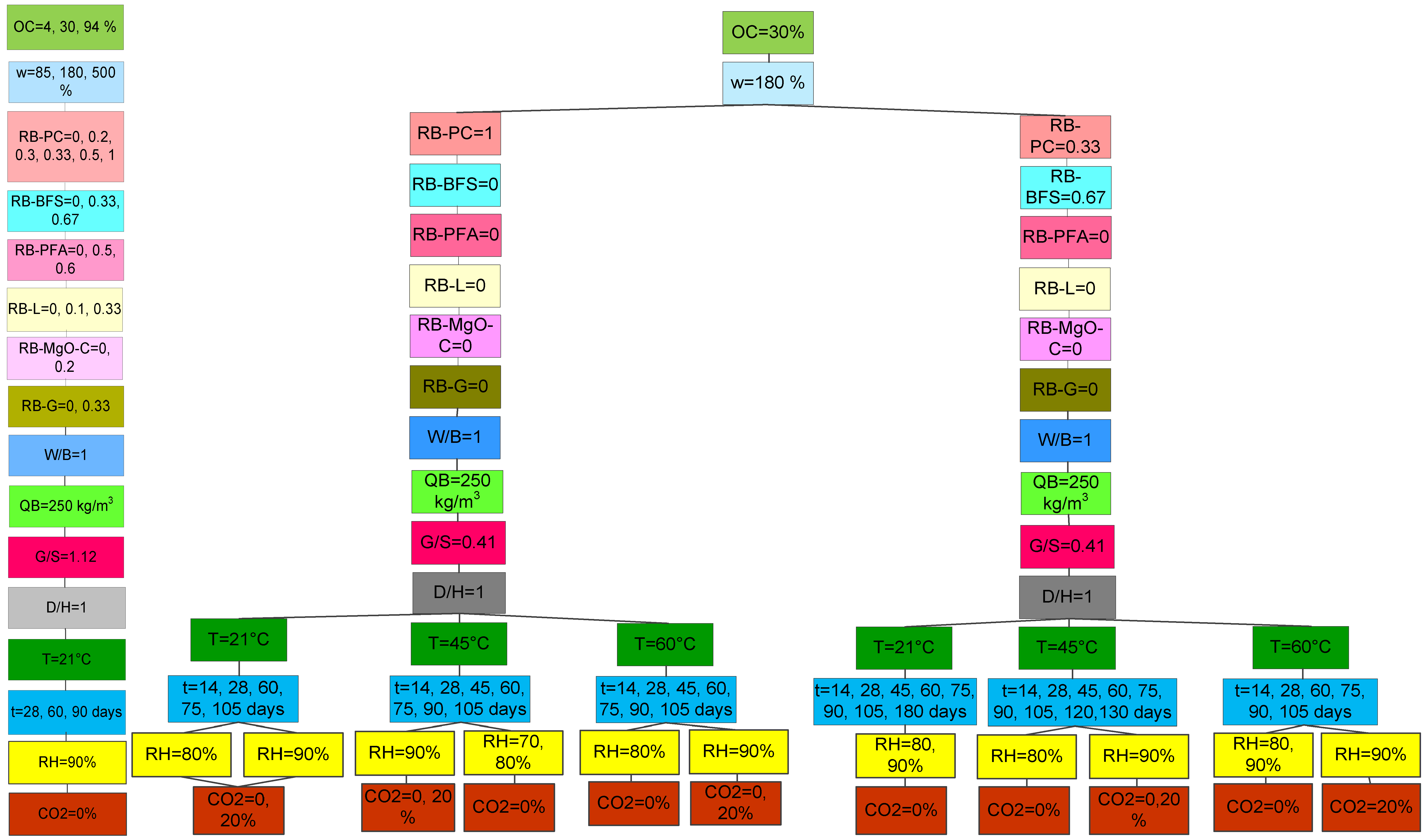
3.1. Experimental Database

Part I of this paper presents the experimental study, the database, and descriptive statistics used for ML analysis [19]. The database included the results of around 1030 unconfined compression tests (339 distinct data records by averaging over the repetitive tests) on three organic soils, including Irish Moss Peat (Pt) with 94% organic content, and two organic clays, OH-1 and OH-2. The OH-1 clay had medium organic content (30%) and extremely high plasticity (LL = 155%), and the OH-2 had low organic content (4%) and high plasticity (LL = 65%). These were combined independently with six mixtures from different binders, including Portland cement (PC), blast furnace slag (BFS), pulverized fuel ash (PFA), lime (L), gypsum (G), and magnesium oxide cement (MgO-C).

Table 1. Characteristics of the organic soils, binders, and mixtures.

Organic Soil	Density (kg/m3)	OC (%)	w (%)
Irish Moss Peat (Pt)	294	94	210
	446		500
	1014		1000
Medium Organic Clay (OH-1)	1219	30	180
Low Organic Clay (OH-2)	1471	4	85

and

Table 2. Binder types and mixtures.

Binders	Binder Mixtures	Ratio
Portland Cement (PC)	PC
Blast Furnace Slag (BFS)	PC + BFS	1:2
Pulverized Fuel Ash (PFA)	PC + PFA	1:1
Lime (L)	PC + PFA + L	3:6:1
Magnesium Oxide Cement (MgO-C)	PC + PFA + MgO-C	2:6:2
Gypsum (G)	L + G + BFS	1:1:1

summarize the organic soils, binders, and mixtures used to prepare the samples [20].

Soil specimens were prepared using a small, concrete-type mechanical mixer. The organic soils and grouts were mixed in the concrete mixer for ten minutes; then, the mix was placed in five layers in a split PVC tube. After the sample preparation process was completed, some of the specimens were cured at a standard ambient temperature (21 °C). Others were placed in a conventional oven and within carbon dioxide (CO₂) incubators at three different temperatures (21 °C, 45 °C, and 60 °C) and three different relative humidity (70%, 80%, and 90%). Samples were cured to varying ages of 14, 28, 60, 90, 105, and 120 days before they were tested.

Table 3. List of control variables and their level/range in the database.

No.	Variables	Range of Variation	Mean	Standard Deviation
Control Variables (Input Parameters)
1	Organic Content of Soil (OC)	4 (OH-2), 30 (OH-1), 94 (Pt) (%)	69.2 (%)	33.2 (%)
2	Water Content of Soil (w)	85, 180, 210, 500, 1000 (%)	400.2 (%)	258.6 (%)
3	Ratio of Binder for Portland Cement (RB-PC)	0, 0.2, 0.3, 0.33, 0.5, 1	0.749	0.339
4	Ratio of Binder for Blast Furnace Slag (RB-BFS)	0, 0.33, 0.67	0.180	0.292
5	Ratio of Binder for Pulverized Fuel Ash (RB-PFA)	0, 0.5, 0.6	0.045	0.154
6	Ratio of Binder for Lime (RB-L)	0, 0.1, 0.33	0.012	0.056
7	Ratio of Binder for Magnesium Oxide (RB-MgO-C)	0, 0.2	0.005	0.032
8	Ratio of Binder for Gypsum (RB-G)	0, 0.33	0.009	0.054
9	Quantity of Binder (QB)	100–500 (kg/m3)	265.9 (kg/m3)	76.6 (kg/m3)
10	Grout to Soil Ratio (G/S)	0.14–3.38	0.856	0.568
11	Water to Binder ratio (W/B)	0.5, 0.8, 1	0.937	0.157
12	Specimen Diameter/Height (D/H)	0.5, 1	0.920	0.183
13	Time (t)	14–180 (days)	61 (days)	36 (days)
14	Temperature (T)	21, 45, 60 (°C)	32.9 (°C)	15.7 (°C)
15	Relative Humidity (RH)	70, 80, 90 (%)	87.6 (%)	4.9 (%)
16	Carbonation (CO2)	0, 20 (%)	2.9 (%)	7.1 (%)
Response Variables (Target Parameters)
	Unconfined Tangent Modulus (E)	0.83–214.62 (MPa)	34.03 (MPa)	31.44 (MPa)
	Unconfined Compression Strength (UCS)	0.04–2.09 (MPa)	0.50 (MPa)	0.40 (MPa)

presents the control and response variables (the strength and stiffness measured from the tests) and their corresponding range of variation in the database. Figure 1 provides a graphical representation of the experimental design.

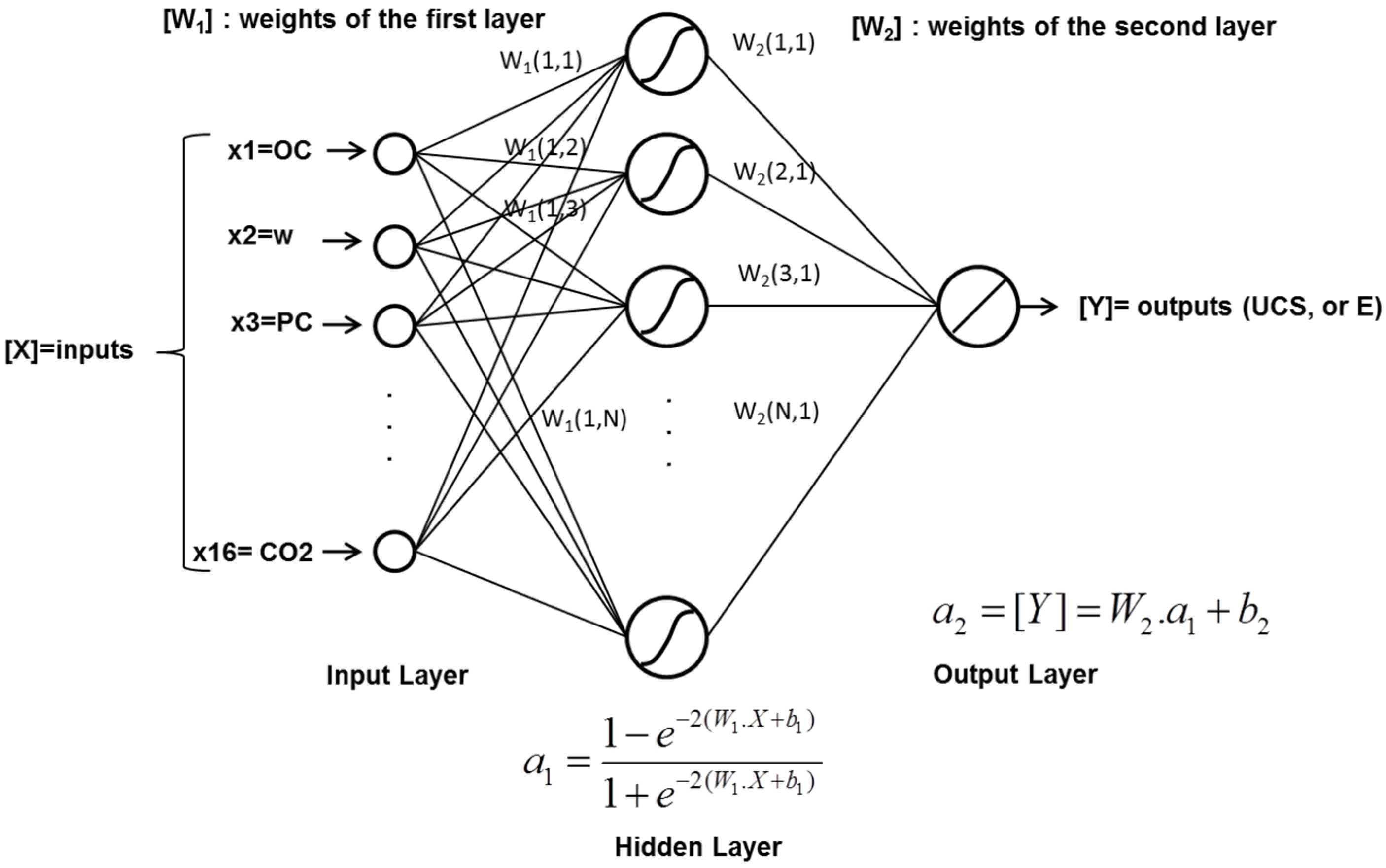
3.2. Artificial Neural Networks

ANNs, first introduced by McCulloch and Pitts [69], have evolved to model regression, classification, and pattern recognition problems with significant computational efficiency. Among various types of ANNs, RBF and MLP are known as “universal approximators” and are commonly used for nonlinear regression modeling [70,71]. These two modeling techniques were applied in this study.

The ANN models’ performance was evaluated using R², the coefficient of determination between measured (actual) and predicted values, and the root mean square of error (RMSE) obtained from the discrepancy between measured and predicted values. To avoid overfitting, a fraction of the database was used to train the ANN models (training subset), and the rest was used to monitor and evaluate the generalization ability of the model (validation and test subsets).

3.2.1. Radial Basis Functions

The RBF network is a feedforward neural network with three layers: the input, hidden, and output layer, as presented in Figure 2. The input layer feeds the input parameters (control variables) into the model. The output layer has one neuron corresponding to the response or output parameter (UCS or E). The function of hidden neurons is to map the input parameters to the output. The basis (transfer/activation) function of the hidden neurons follows a Gaussian form [70,71]:

$$\phi (X)=e^{(-\frac{{\Vert X-C\Vert }^2}{2{\sigma }^2})}$$

(1)

where X is the input vector, and C is the vector determining the center of the basis functions. σ is the parameter that specifies the spread of the basis functions and controls interpolation’s smoothness.

The RBF network uses the fixed center learning strategy, i.e., the hidden neurons’ centers are defined as the input vectors in the training dataset. Therefore, the number of hidden units is equal to the size of the training dataset. The final output function of the network can be written as follows:

$$Y=W{e}^{-{(\Vert X-C\Vert b_1)}^2}+b_2$$

(2)

where

Y = output matrix (model response);

W = weight matrix (model parameters);

X = input matrix (predictor variables);

C = centers of Gaussian functions;

$b_1=\frac{1}{\sigma \sqrt{2}}$ = spread of the Gaussian function (hyperparameter);

$b_2$ = bias vector of the output layer (hyperparameters).

If it is assumed that $b_2=0$, then the RBF network provides an interpolating function that passes through all the data points. Such a function is overfitted, and therefore highly oscillatory [70]. Thus, the bias parameter is introduced to smooth the interpolation and improve the generalization of the model.

The proposed network was evaluated for various values of $b_1$. The value that minimized the error on the test dataset was eventually selected as the standard deviation of the Gaussian functions. The weights of the second layer were calculated to minimize the error function (the sum of squared errors) given by:

$$E=\frac{1}{2}{\displaystyle \sum _n{\displaystyle \sum _k^{}{(y_k(x^n)-t_k^n)}^2}}$$

(3)

where $t_k^n$ is the target value of the unit k, corresponding to the input vector $x_{}^n$. Minimizing the error function of Equation (3) leads to solving a set of linear equations:

$$\begin{array}{l}\Phi W^{\mathrm{T}}=T\\ W^{\mathrm{T}}={({\Phi }^{\mathrm{T}}\Phi )}^{-1}{\Phi }^{\mathrm{T}}d\end{array}$$

(4)

where, $\Phi$ is the output of the hidden layer, and $T$ is the target matrix containing $t_k^n$ elements.

Ensembles of networks were generated by the random subsampling method, also known as the Monte Carlo sampling method [72]. The RBF network was trained from scratch a large number of times (1000). Each time, the database was randomly divided into training and test subsets (4:1 ratio), and a new network was generated and trained, starting from a random initial set of weights, forming an ensemble of networks. The networks learned from the data points in the training datasets, and their generalization was examined through the test datasets. The ensembles’ performance was evaluated using the average R² (R²_ave) and RMSE (RMSE_ave).

3.2.2. Multilayer Perceptron

The MLP network architecture is presented in Figure 3. It consists of three layers, including the input layer, the hidden layer with N neurons, and the output layer. Hidden neurons in MLP networks apply threshold or sigmoid activation functions. A preliminary analysis was performed to select the appropriate type of sigmoid function. Based on this analysis, tan-sigmoid and log-sigmoid functions resulted in about the same prediction accuracy. However, tan-sigmoid slightly outperformed the log-sigmoid function. In general, tan-sigmoid activation functions are known to result in faster convergence compared to log-sigmoid functions. The tan-sigmoid activation function used for the MLP network is defined as [70,71]:

$$\phi (X)=\tanh (X)=\frac{e^X-e^{-X}}{e^X+e^{-X}}$$

(5)

The output layer has one neuron associated with the response variable. The output function of the network can be formulated as:

$$Y=W_2\frac{1-e^{-2(W_{1}X+b_1)}}{1+e^{-2(W_{1}X+b_1)}}+b_2$$

(6)

where

Y = output matrix (model response).

W₁ = weight matrix of the hidden layer (model parameters).

W₂ = weight matrix of the output layer (model parameters).

X = input matrix (predictor variables).

b₁ = bias vector of the hidden layer (hyperparameters).

b₂ = bias vector of the output layer (hyperparameters).

The weights are adjusted following a backpropagation algorithm (BP). The learning process consists of conducting two rounds of computation for each iteration: a forward error computation and a backward error backpropagation. The mean squared error is computed based on the discrepancy between output and target vectors in the forward pass. The network weights get adjusted layer by layer in the backward pass, based on an optimization algorithm (such as gradient descent, Levenberg–Marquardt, etc.).

The Levenberg–Marquardt (LM) optimization algorithm is known to outperform the conventional gradient descent methods [70,71] and was implemented for the MLP networks in this study. The database was split into three groups: training, validation, and test (3:1:1 ratio). Network weights were adjusted during training while the performance was being monitored over the validation dataset. This learning process continued until the network error began to increase over the validation dataset or until it reached a certain threshold (usually 0.1–0.01). The random subsampling method was used to generate ensembles of MLPs. Additionally, to assess the optimum number of hidden neurons, a sensitivity analysis was performed by varying the number of hidden neurons from 5 to 100.

3.2.3. Multiple Linear Regression (MLR)

MLR models were also developed to compare with the two ANN models described earlier. The proposed MLR model is formulated as [73]:

$$Y={\beta }_0+{\beta }_1{X}_1+\cdots +{\beta }_n{X}_n=\widehat{\beta }X$$

(7)

where

Y = output matrix (model response).

β₀, …, β_n = regression coefficients (model parameters).

X = input matrix (predictor variables).

Regression coefficients were computed using the least squares method (LSM).

All the computations in this study were performed by MATLAB [74].

4. Analysis and Results

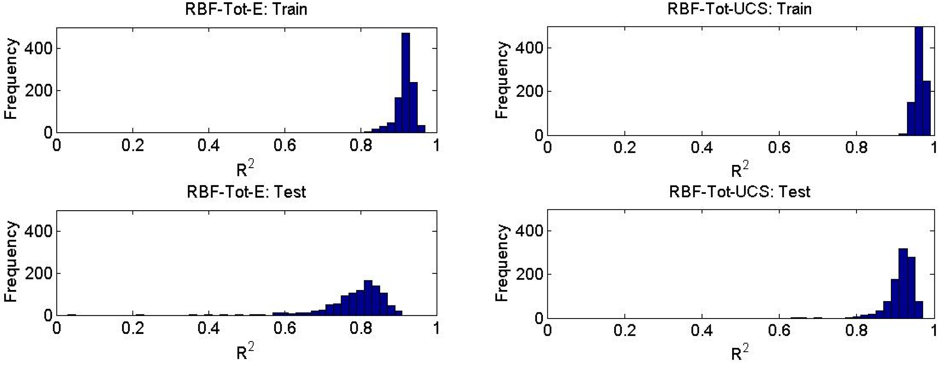
4.1. RBF Network Analysis

ANN models showed considerable improvement in performance after data normalization. Therefore, the normalized experimental database was used to train the ANN models.

Table 4. Performance of RBF models for E and UCS.

Model	All		Training		Test
	R2ave	RMSEave	R2ave	RMSEave	R2ave	RMSEave
RBF-Tot-E	0.89	2.78	0.92	0.03	0.77	13.77
RBF-Tot-UCS	0.95	0.09	0.96	0.08	0.92	0.11

presents a summary of the prediction results. R²ave over the test datasets is close to 0.8 for the prediction of E and above 0.9 for the prediction of UCS. Additionally, the RMSE is 13 MPa for E and 0.11 MPa for UCS. These results show that RBF models successfully captured the correlations between the control and the response variables within the training dataset and generalized the captured trends to the test dataset with acceptable accuracy. RBF models show better performance for the prediction of UCS compared to E.

Figure 4 shows the distribution of R² values corresponding to the networks of the ensemble (RBF-Tot). As expected, the uncertainty of predictions over the training dataset is significantly lower than the test dataset. Additionally, the uncertainty of predictions for E is substantially higher than for UCS.

4.2. MLP Network Analysis

According to [70], for MLPs with continuous nonlinear hidden-layer activation functions, one hidden layer with an arbitrarily large number of units suffices for any approximation. However, there are no rules for determining the optimum number of neurons in a hidden layer. Typically, it is recommended to keep the number of hidden neurons between the number of input elements and the number of output elements, but not greater than twice the number of input elements [70]. Too few hidden neurons increase the prediction error and prevent the ANN model from having enough flexibility to fit the data points. On the other hand, too many hidden neurons would make the model overfit the data and therefore fail to generalize [75].

Trenn [76] suggests the following formulation for the minimum number of hidden units for a single hidden layer network to reach a specific order of approximation:

$$n=\frac{\left(\begin{array}{l}N+n_0\\ n_0\end{array}\right)}{n_0+2}$$

(8)

where

n = Minimum number of hidden units;

N = Order of approximation;

n₀ = Number of input variables.

N refers to the degree of Taylor polynomials approximating the MLP function. For instance, to have an approximation of N = 2 in this problem (with 16 input variables), at least nine hidden neurons are required.

Figure 5 shows the variation of R² with respect to the number of hidden neurons. The optimum number of hidden neurons is 20 for predicting E and 25 for predicting UCS.

The performance of the MLP models is summarized in

Table 5. Performance of MLP models for E and UCS.

Model	All		Training		Validation		Test
	R2ave	RMSEave	R2ave	RMSEave	R2ave	RMSEave	R2ave	RMSEave
MLP-20-E	0.81	13.58	0.95	6.15	0.50	20.74	0.61	18.47
MLP-25-UCS	0.90	0.12	0.99	0.04	0.73	0.20	0.80	0.17

. The average R² over the test dataset is 0.8 for UCS and 0.61 for E. The average RMSE is 18 MPa for E and 0.17 MPa for UCS, showing a reasonably good level of prediction accuracy (especially for UCS). Figure 6 presents the distribution of the R² associated with the networks of the MLP ensembles. As expected, and consistent with the RBF models’ results, the uncertainty of predictions over the training datasets was much lower compared to the other subsets. Additionally, the uncertainty of predictions for UCS was less than E.

The RBF models outperformed the MLPs, showing 35% less error for the prediction of E and 40% less error for the prediction of UCS.

4.3. Stepwise Parameter Selection for ANNs

A stepwise parameter selection method was implemented to identify the most significant parameters for the mechanical properties of stabilized organic soils [77]. This method reduces the ANN model dimensionality and optimizes the overall performance by identifying the highly correlated input parameters and removing the redundant ones.

This method includes forward stepwise selection (FSS) and backward stepwise elimination (BSE) of the input parameters, based on their significance to the network’s prediction accuracy. At each step, an ensemble of networks is trained using a control subset of the database (including 80% of the whole database). In forward stepwise selection, parameters compete to be added one by one to the model. A parameter is added to the model only if the adjusted R² for the model becomes larger than the adjusted R² of the reduced model. In the backward elimination, the process starts with a network containing all input parameters, and the parameters are gradually removed one by one. A parameter is removed when the adjusted R² for the reduced model becomes larger than the present model.

Adjusted R² provides the possibility of penalizing the model for the number of input parameters and is calculated based on the following equation:

$$R^2{}_{adj}=\frac{(n-1)R^2-p}{n-1-p}$$

(9)

where

R²_adj = adjusted value.

n = no. of data points presented to the network in the training dataset.

R² = R² for the reduced model.

p = no. of model parameters (weights and biases) for the reduced model.

Table 6. Stepwise selection of parameters, RBF network.

	RBF-E			RBF-UCS
Order of Addition/Elimination	FSS	BSE	Ranking/Sequence of Addition	FSS	BSE	Ranking/Sequence of Addition
1	Binder Type	w	Binder Type	G/S	W/B	G/S
2	G/S	OC	G/S	Binder Type		Binder Type
3	t	QB	t	t		t
4	D/H	W/B	D/H	T		T
5	T		T	RH		RH
6	RH		RH	CO2		CO2
7	CO2		CO2	D/H		D/H
8			w			w
9			OC			OC
10			QB			QB
11			W/B			W/B

and

Table 7. Stepwise selection of parameters, MLP network.

	MLP-E			MLP-UCS
Order of Addition/Elimination	FSS	BSE	Ranking/Sequence of Addition	FSS	BSE	Ranking/Sequence of Addition
1	Binder Type	W/B	Binder Type	G/S	QB	G/S
2	G/S		G/S	Binder Type		Binder Type
3	t		t	t		t
4	D/H		D/H	T		T
5	T		T	RH		RH
6	RH		RH	CO2		CO2
7	CO2		CO2	W/B		W/B
8	QB		QB	D/H		D/H
9			w	QB		QB
10			OC	OC		OC
11			W/B			w

present the selected and removed parameters using the forward and backward stepwise methods for the RBF and MLP models, respectively. The parameters were ranked based on their sequence of addition to the model, which represented their significance to the model performance. For ranking, the parameter addition process was continued even after the R²_adj of the reduced model started to decrease. After this stage, the parameter that resulted in the smallest decrease in R²_adj was added to the model at each step. This continued until all the parameters were added to the model.

Based on the FSS method, w, OC, QB, and W/B were parameters that could be removed from the RBF model for the prediction of UCS. However, based on the BSE method, only W/B could be eliminated. The same parameters were selected for the prediction of E, but the parameters’ ranking was slightly different.

The FSS method added all the parameters to the MLP model for UCS prediction, except for w. The BSE method only removed QB. For the prediction of E, the FSS method did not add w, OC, or W/B to the MLP. W/B was the only parameter eliminated from the model by the BSE method.

The final selected parameters were different for the RBF and MLP models. However, the parameters chosen by both the FSS and BSE methods for the MLP model covered those chosen by the RBF model. Additionally, the resulted ranking of parameters was similar for both MLP and RBF.

QB is known to directly influence cemented soils’ stiffness and strength [78]; however, the stepwise selection method suggested removing it from the model. From the cross-correlation of the input and target parameters (see

Table 8. Cross-correlation between input and target parameters (high correlations shown in bold).

	OC	w	PC	BFS	PFA	L	MgO-C	G	QB	G/S	W/B	D/H	t	T	RH	CO2	E	UCS
OC	1.00	0.69	0.32	−0.17	−0.23	−0.16	−0.13	−0.13	0.16	0.61	−0.30	−0.33	−0.07	−0.16	0.11	−0.09	0.08	0.19
w		1.00	0.26	−0.17	−0.16	−0.12	−0.09	−0.09	0.14	0.00	−0.81	−0.29	−0.05	−0.17	0.11	−0.10	−0.19	−0.09
PC			1.00	−0.79	−0.37	−0.42	−0.27	−0.36	0.15	0.18	−0.30	−0.32	−0.07	−0.13	−0.01	−0.02	0.18	0.30
BFS				1.00	−0.18	0.05	−0.10	0.08	−0.13	−0.11	0.25	0.27	0.00	0.33	−0.11	0.12	−0.07	−0.14
PFA					1.00	0.13	0.60	−0.05	−0.06	−0.12	0.12	0.13	0.10	−0.22	0.14	−0.12	−0.16	−0.27
L						1.00	−0.03	0.95	−0.04	−0.08	0.08	0.09	0.07	−0.16	0.10	−0.09	−0.13	−0.15
MgO−C							1.00	−0.03	−0.03	−0.07	0.07	0.07	0.05	−0.13	0.08	−0.07	−0.08	−0.16
G								1.00	−0.03	−0.07	0.07	0.07	0.05	−0.13	0.08	−0.07	−0.10	−0.11
QB									1.00	0.46	−0.28	−0.19	−0.01	−0.16	0.10	−0.09	0.40	0.59
G/S										1.00	0.22	−0.20	−0.05	−0.12	0.08	−0.07	0.45	0.56
W/B											1.00	0.37	0.02	0.30	−0.20	0.17	0.16	0.02
D/H												1.00	0.02	0.33	−0.21	0.18	0.11	−0.21
t													1.00	−0.03	0.02	−0.01	0.09	0.11
T														1.00	−0.31	0.35	−0.21	−0.29
RH															1.00	0.20	−0.02	0.05
CO2																1.00	−0.08	−0.09

), it is observed that G/S and QB show a relatively high correlation (r = 0.46), i.e., the G/S variable could represent QB to some extent. Additionally, OC is removed by the FSS method due to the high correlation with G/S (r = 0.61). As observed from Figure 1, for OC = 94%, G/S ranges between 0.14 to 3.38. For OC = 30, G/S is 0.41, and for OC = 4%, G/S is 1.12. Either W/B or w (or both) was eliminated due to limited significance in the presence of other relevant parameters. W/B is equal to 1 for most experiments; therefore, there is not much variability in W/B to influence E and UCS predictions. Additionally, there is a high negative correlation (–0.81) between W/B and w, per Table 8, as for lower initial water content, a higher ratio of water to binder was used.

4.4. Linear Regression Analysis

For the MLR model development, the database was divided into training and test datasets with a 4:1 ratio. An ensemble of models (1000 models) was generated using the random subsampling method, similarly to the ANN models.

Table 9. Performance of the LR ensemble for E and UCS.

Model	R2ave			RMSEave
	All	Training	Test	All	Training	Test
LR-E	0.49	0.51	0.42	22.33	22.04	23.48
LR-UCS	0.66	0.67	0.62	0.23	0.23	0.25

presents the performance of the MLR ensemble models. The prediction accuracy of the MLR models is significantly lower than the ANN models, showing R²ave of 0.42 for E and 0.62 for UCS over the test datasets.

4.5. Model Comparison

The three ML models (RBF, MLP, and MLR) were further evaluated and compared over a fraction of the database that was not previously used for training, incorporating only the input parameters selected by the stepwise method.

Figure 7 presents the measured vs. predicted E and UCS by the three models. Both the RBF and MLP models outperformed the MLR model, showing R² > 0.95. The MLR model shows a significantly lower R², 0.64 for prediction of E, and 0.73 for UCS.

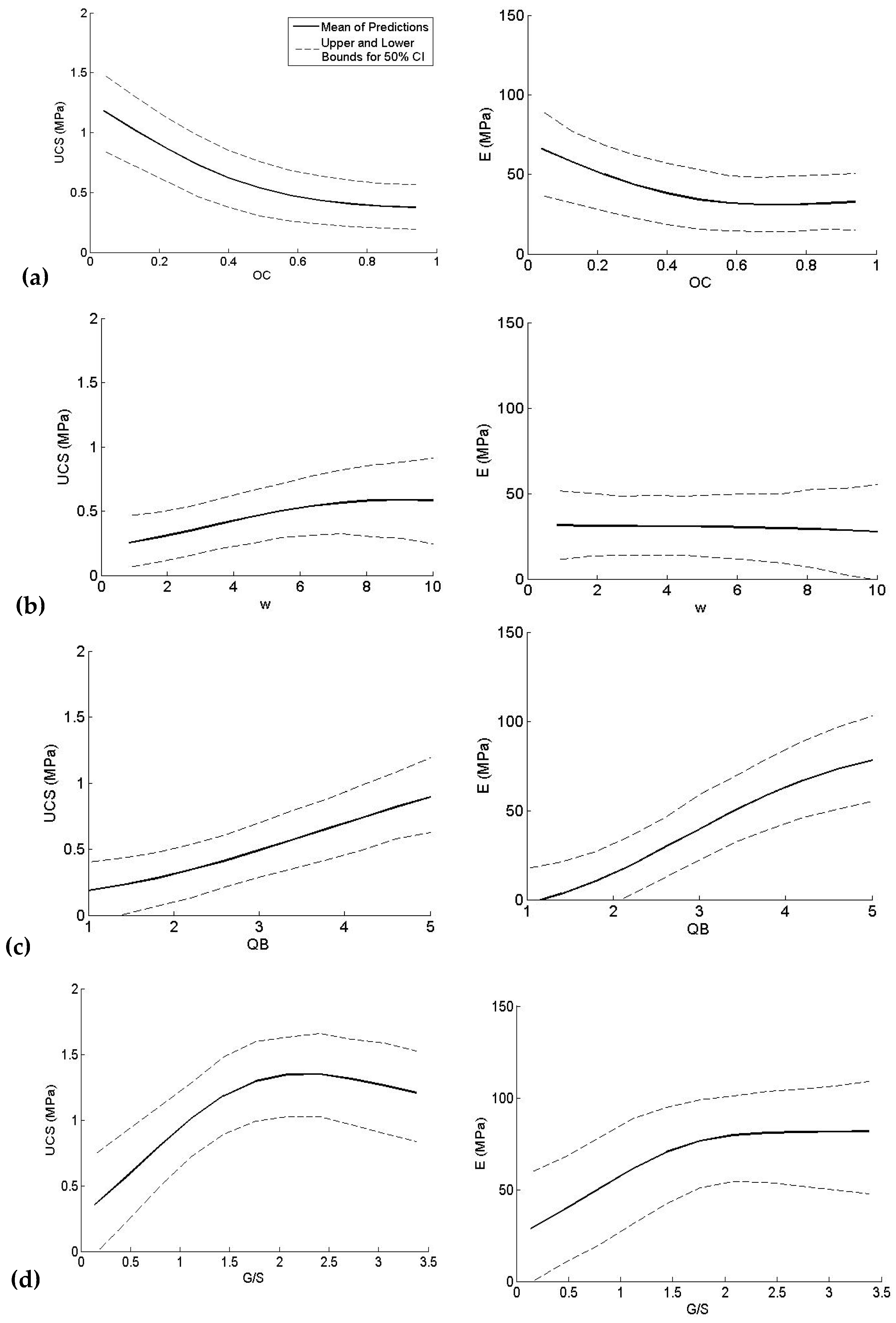
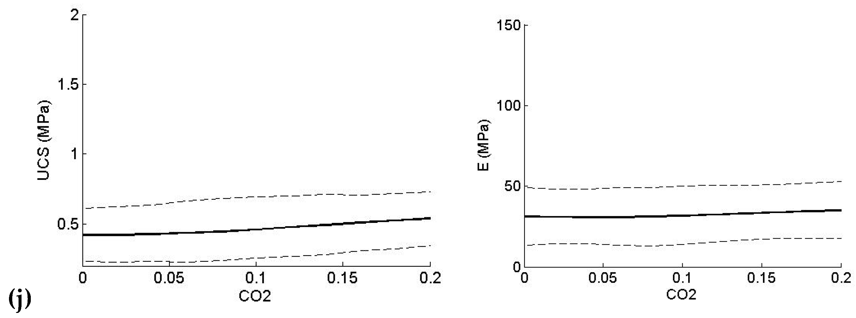
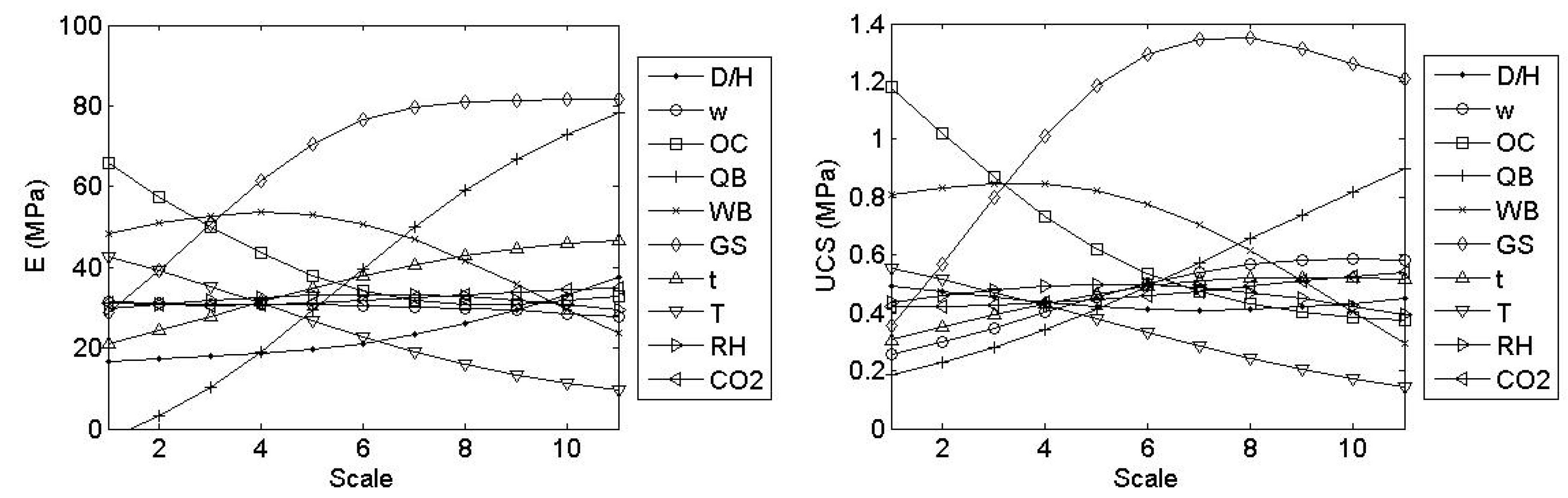
4.6. Sensitivity Analysis

The impacts of control variables on the predicted E and UCS were evaluated using a sensitivity analysis method known as the profile method [79]. This method evaluates the sensitivity of ANN models to each input parameter and captures the variation trend between the model response and each parameter. The generated profile graphs, as shown in Figure 8, capture the optimum range of each parameter to achieve the maximum strength and stiffness.

A set of fictitious matrices was constructed corresponding to each input variable (except for the binder ratio). All other input variables were held constant at their mean value, whereas the studied parameter varied over its range. The range of variation was divided into ten intervals, and the model response was evaluated at each point. Note that the binder ratio’s effect was not explored in this analysis because it was not possible to vary one binder type ratio while keeping the ratio of the other types constant (the sum of the binder ratios for the six binder types should be equal to 1). Thus, for each parameter, 11 input vectors were presented to the models that resulted in 11 responses compiling the response graph for that parameter.

The MLP-20-E and MLP-25-UCS models were used for generating the response graphs. The response graphs present the average of predictions from 1000 networks in the MLP ensembles. The upper and lower bounds correspond to the 50% confidence interval (CI) of the model predictions. While interpreting these graphs for a parameter, one should consider the mean value for all other input parameters (see Table 3).

The following observations are made from the response graphs:

• An increase in OC significantly decreases E and UCS, as confirmed by other studies [1,2,80].
• UCS shows a slight increase with w, reaching maximum at a range between 800% to 1000%, opposing the generally expected trend. Such a trend has occurred primarily in the field when the initial water content is very low, also when adding large quantities of dry binders that prevent proper mixing and hydration [81].
• Both E and UCS increase with an increase in QB, as confirmed by other studies [78].
• Increasing G/S increases both E and UCS up to a certain value. In this analysis, the optimum range for G/S is between 2 and 2.5.
• The optimum range for W/B is between 0.6 to 0.7, and larger values of W/B cause a considerable decrease in E and UCS.
• D/H does not show a significant impact on UCS; however, E shows to increase with D/H slightly.
• Age of the specimen is positively correlated with E and UCS. E and UCS rapidly increase during the first 90 days (a time when much of the hydration process developed). After that, the rate of increase decays.
• Both E and UCS decay with an increase in curing temperature (T), opposing the behavior of common stabilized mineral soils, where the temperature increases the strength and stiffness. The negative effect of temperature on the stiffness and strength of organic soils is related to several factors, such as gradual loss of the initial evaporable water in the mix, dehydration during chemical reactions, and porosity changes [20].
• RH = 0.8 is shown to be the optimum value for both E and UCS, although the overall trend suggests that relative humidity is not a significant parameter.
• CO₂ shows a minimal effect on E and UCS, with a slight developing trend observed for UCS.

The response graphs versus the scale of variation (1 to 11) for each control variable are presented in Figure 9. The ranking of the variables (ANN input parameters) was determined by comparing E and UCS range of variations within the domain of each variable, representing their order of significance to the stiffness and strength of stabilized organic soils (see

Table 10. Ranking of the control variables (input parameters) based on the sensitivity analysis using the profile method.

Ranking	Parameter	Max. E Variation (MPa)	Parameter	Max. UCS Variation (MPa)
1	QB	80.59	G/S	0.99
2	G/S	53.07	OC	0.81
3	OC	34.97	QB	0.71
4	T	32.91	W/B	0.55
5	W/B	29.93	T	0.41
6	t	25.61	w	0.33
7	D/H	20.88	t	0.22
8	CO2	4.25	CO2	0.12
9	RH	3.94	RH	0.10
10	w	3.74	D/H	0.08

).

5. Conclusions

Understanding the behavior of stabilized organic soils, the optimal design of soil binder mixture, and the range of achieved strength and stiffness for organic soils is crucial for practical applications in engineering design and construction, a topic not yet fully addressed in the existing literature. This study presents a novel application of ML methods to develop robust, nonlinear predictive models for mechanical properties of stabilized organic soils and to evaluate the impacts of control variables such as soil, binder, and mixture parameters, and other relevant experimental and environmental factors on these properties. The most influential parameters were identified, and the nonlinear trend of stiffness and strength with these parameters were developed through highly accurate ANN models.

Ensembles of RBF, MLP, and MLR models were developed to predict the stiffness and strength of stabilized organic clays, with a wide range of organic content and a variety of binder mixes. RBF networks showed the highest predictive accuracy, followed closely by MLP. As anticipated, the linear regression method demonstrated a significantly lower prediction accuracy than both ANN methods. ANN models predicted E and UCS with a high accuracy level (R² > 0.8 for E and R²> 0.9 for UCS). The most relevant input parameters for ANN models were identified through the stepwise parameter selection method, and the redundant parameters were eliminated.

The impacts of input parameters on the stiffness and strength and each parameter’s optimum range were evaluated through ANN sensitivity analyses. The generated response graphs showed how ANNs could account for the nonlinear relations between the mechanical properties of stabilized organic soils and the control variables. The input parameters were ranked using both the stepwise selection and the sensitivity analysis method. Grout to soil ratio/quantity of binder, binder mix type, organic content, water to binder ratio, temperature, and time (aging) were identified as the most influential parameters. The specimen size barely affected UCS, with a slight influence on E. Therefore, for application in design (where there is no specimen size), any values between 0.5 to 1 can be assumed, or the specimen size can be removed from the list of input parameters. Carbonation and relative humidity showed less impact on both E and UCS, indicating the need to study the long-term behavior of stabilized organic soils in more detail. ANNs significantly outperformed the conventional linear regression methods, which are often used in practice to estimate the stiffness and strength of stabilized soils.

Compared to other existing studies that have applied ML for investigating the stabilized soils (see Section 2), the novel contributions of this study are summarized below:

• Part I and II of this study together provide comprehensive details and descriptions of both experimental and computational investigations. Unlike most of the other studies, the experiments were designed to generate a well-populated database suitable for application of ML. This is essential for developing robust, reliable predictive models on any experimental database. Full access to the database and descriptive statistics are provided in Part I.
• The mechanical behavior of stabilized organic soils has not been comprehensively addressed by other studies. In this study, using a hybrid experimental and ML approach, the stiffness and strength as the two critical engineering design parameters were investigated, and the impacts of the relevant factors on the stiffness and strength of stabilized organic soils were evaluated.
• This study investigated various types of soils (low and high plasticity clays) and binders (both cement and non-cement based).
• Using a novel ML approach, the most influential parameters (control variables) were identified, the trends of strength and stiffness variation with these parameters (with 50% CI) were developed, and the optimum ranges were identified, allowing for an optimal mixture design.
• The two most prominent ANN algorithms were successfully applied to predict the stiffness and strength, and the full details of the architecture development and training methods were provided. Comparing their performance with other ML methods recently applied in other studies showed that these ANN algorithms are still highly competent.

Overall, the proposed ML approach can be instrumental for optimal mixture design and minimizing the experimental cost of implementing DSM in engineering projects involving organic soils. Additionally, this paper can serve as a guideline for rigorous predictive modeling and parametric analysis using ML based on experimental data.

References

1. Edil, T.N.; Den Haan, E.J. Settlement of Peats and Organic Soils Settlement; ASCE Geotechnical Special Publication: Boston, MA, USA, 1994; Volume 4, pp. 1543–1572. [Google Scholar]
2. Kruse, G.; Haan, E.D. Characterisation and Engineering Properties of Dutch Peats Characterisation and Engineering Properties of Natural Soils; Taylor & Francis: Abingdon, UK, 2006. [Google Scholar]
3. Hampton, M.B.; Edil, B. Strength gain of organic ground with cement-type binders. In Soil Improvement for Big Digs, Proceedings of the Geo-Congress ’98, Boston, MA, USA, 18–21 October 1998; ASCE Geotechnical Special Publication: New York, NY, USA, 1998. [Google Scholar]
4. Hayashi, H.; Nishimoto, S. Strength characteristics of stabilized peat using different types of binders. In Proceedings of the International Conference on Deep Mixing Best Practice and Recent Advances, Stockholm, Sweden, 23–25 May 2005; Deep Stabilization Research Centre: Stockholm, Sweden, 2005; Volume 1.1, pp. 55–62. [Google Scholar]
5. Jelisic, N.; Leppanen, M. Mass stabilisation of organic soils and soft clay. In Proceedings of the Grouting and Ground Treatment: Proceedings of the Third International Conference, New Orleans, LA, USA, 10–12 February 2003; ASCE: Reston, VA, USA, 2003; pp. 552–561. [Google Scholar]
6. Lambrechts, J.R.; Ganse, M.A.; Layhee, C.A. Soil Mixing to Stabilize organic Clay for I-95 Widening. In Proceedings of the third International Conference in Grouting and Ground Treatment, New Orleans, LA, USA, 10–12 February 2003; ASCE: New Oreans, LA, USA, 2003; pp. 575–585. [Google Scholar]
7. Chew, S.H.; Kamruzzaman, A.H.M.; Lee, F.H. Physicochemical and engineering behavior of cement treated clays. J. Geotech. Geoenviron. Eng. 2004, 130, 7696–7706. [Google Scholar] [CrossRef]
8. Consoli, N.C.; Cruz, R.C.; Floss, M.F.; Festugato, L. Parameters controlling tensile and compressive strength of artificially cemented sand. J. Geotech. Geoenviron. Eng. 2010, 136, 759–763. [Google Scholar] [CrossRef]
9. Consoli, N.C.; da Fonseca, A.V.; Cruz, R.C.; Heineck, K.S. Fundamental parameters for the stiffness and strength control of artificially cemented sand. J. Geotech. Geoenviron. Eng. 2009, 135, 1347–1353. [Google Scholar] [CrossRef] [Green Version]
10. Consoli, N.C.; Foppa, D.; Festugato, L.; Heineck, K.S. Key parameters for strength control of artificially cemented soils. J. Geotech. Geoenviron. Eng. 2007, 133, 197–205. [Google Scholar] [CrossRef]
11. Kitazume, M. Technical session 2a: Ground improvement. In Proceedings of the 16th International Conference on Soil Mechanics and Geotechnical Engineering, Osaka, Japan, 12–16 September 2005; Milpress: Rotterdam, The Netherlands, 2005; Volume 1–5, pp. 3011–3020. [Google Scholar]
12. Porbaha, A. Design aspects and properties of treated ground. In Proceedings of the Deep Mixing Workshop, Geo-Trans, Los Angeles, CA, USA, 27–31 July 2004. [Google Scholar]
13. Schnaid, F.; Prietto, P.D.M.; Consoli, N.C. Characterization of cemented sand in triaxial compression. J. Geotech. Geoenviron. Eng. 2001, 127, 857–868. [Google Scholar] [CrossRef]
14. Grubb, D.G.; Chrysochoou, M.; Smith, C.J.; Malasavage, N.E. Stabilized dredged material. I: Parametric study. J. Geotech. Geoenviron. Eng. 2010, 136, 1011–1024. [Google Scholar] [CrossRef]
15. Grubb, D.G.; Malasavage, N.E.; Smith, C.J.; Chrysochoou, M. Stabilized dredged material. II: Geomechanical behavior. J. Geotech. Geoenviron. Eng. 2010, 136, 1025–1036. [Google Scholar] [CrossRef]
16. Huttunen, E.; Kujala, K. On the stabilization of organic soils. In Proceedings of the Second International Conference on Ground Improvement Geosystems, Tokyo, Japan, 14–17 May 1996; Balkema: Rotterdam, The Netherlands, 1996; pp. 411–414. [Google Scholar]
17. Tremblay, H.; Duchesne, J.; Locat, J.; Leroueil, S. Influence of the nature of organic compounds on fine soil stabilization with cement. Can. Geotech. J. 2002, 39, 535–546. [Google Scholar] [CrossRef]
18. MMcGinn, A.J.; O’Rourke, T.D. Performance of Deep Mixing Methods at Fort Point Channel; Cornell University: Ithaca, NY, USA, 2003. [Google Scholar]
19. Hernandez-Martinez, F.G.; Al-Tabbaa, A.; Medina-Cetina, Z.; Yousefpour, N. Stiffness and Strength of Stabilized Organic Soils—Part I/II: Experimental Database and Statistical Description for Machine Learning Modeling. Application of Artificial Intelligence and Machine Learning in Geotechnical Engineering. Geosciences 2021. [Google Scholar]
20. Hernandez-Martinez, F.G. Ground Improvement of Organic Soils Using Wet Deep Soil Mixing. Ph.D. Thesis, University of Cambridge, Cambridge, UK, 2006. [Google Scholar]
21. Yousefpour, N.; Fallah, S. Applications of Machine Learning in Geotechnics. In Proceedings of the Civil Engineering Research in Ireland Conference, Dublin, Ireland, 29–30 August 2018. [Google Scholar]
22. Goh, A.T.C. Nonlinear modelling in geotechnical engineering using neural networks. Aust. Civ. Eng. Trans. CE 1994, 36, 293–297. [Google Scholar]
23. Goh, A.T.C. Empirical design in geotechnics using neural networks. Empir. Des. Geotech. Neural Netw. 1995, 45, 709–714. [Google Scholar] [CrossRef]
24. Goh, A.T.C. Pile driving records reanalyzed using neural networks. J. Geotech. Geoenviron. Eng. 1996, 122, 492. [Google Scholar] [CrossRef]
25. Chow, Y.K.; Chan, W.T.; Liu, L.F.; Lee, S.L. Prediction of pile capacity from stress-wave measurements: A neural network approach. Int. J. Numer. Anal. Meth. Geomech. 1995, 19, 107–126. [Google Scholar] [CrossRef]
26. Lee, I.-M.; Lee, J.-H. Prediction of pile bearing capacity using artificial neural networks. Comput. Geotech. 1996, 18, 189–200. [Google Scholar] [CrossRef]
27. Goh, A.T.C.; Kulhawy, F.H.; Chua, C.G. Bayesian neural network analysis of undrained Side resistance of drilled shafts. J. Geotech. Geoenviron. Eng. 2005, 131, 84–93. [Google Scholar] [CrossRef]
28. Pal, M.; Deswal, S. Modeling pile capacity using support vector machines and generalized regression neural network. J. Geotech. Geoenviron. Eng. 2008, 134, 1021–1024. [Google Scholar] [CrossRef]
29. Zhang, W.; Goh, A.T.C. Multivariate adaptive regression splines and neural network models for prediction of pile drivability. Geosci. Front. 2016, 7, 45–52. [Google Scholar] [CrossRef] [Green Version]
30. Shahin, M.A. State-of-the-art review of some artificial intelligence applications in pile foundations. Geosci. Front. 2016, 7, 33–44. [Google Scholar] [CrossRef] [Green Version]
31. Ellis, G.W.; Yao, C.; Zhao, R.; Penumadu, D. Stress-strain modeling of sands using artificial neural networks. J. Geotech. Geoenviron. Eng. 1995, 121, 429–435. [Google Scholar] [CrossRef]
32. Ghaboussi, J.; Sidarta, D.E. New nested adaptive neural networks (NANN) for constitutive modeling. Comput. Geotech. 1998, 22, 29–52. [Google Scholar] [CrossRef]
33. Penumadu, D.; Jean-Lou, C. Geomaterial modeling using artificial neural networks. In Artificial Neural Networks for Civil Engineers: Fundamentals and Applications; ASCE: Reston, VA, USA, 1997; pp. 160–184. [Google Scholar]
34. Penumadu, D.; Zhao, R. Triaxial compression behavior of sand and gravel using artificial neural networks (ANN). Comput. Geotech. 1999, 24, 207–230. [Google Scholar] [CrossRef]
35. Das, S.K.; Basudhar, P. Prediction of residual friction angle of clay artificial neural network. Eng. Geol. 2008, 100, 142–145. [Google Scholar] [CrossRef]
36. Obrzud, R.F.; Vulliet, L.; Truty, A. A combined neural network/gradient-based approach for the identification of constitutive model parameters using self-boring pressuremeter tests. Int. J. Numer. Anal. Meth. Geomech. 2009, 33, 817–849. [Google Scholar] [CrossRef]
37. Khan, S.Z.; Suman, S.; Pavani, M.; Das, S.K. Prediction of the residual strength of clay using functional networks. Geosci. Front. 2016, 7, 67–74. [Google Scholar] [CrossRef] [Green Version]
38. Rizzo, D.M.; Lillys, T.P.; Dougherty, D.E. Comparisons of site characterization methods using mixed data. In Uncertainty in the Geologic Environment: From Theory to Practice; Geotechnical Special Publication; ASCE: Reston, VA, USA, 1996; Volume 58, pp. 157–179. [Google Scholar]
39. Tsiaousi, D.; Travasarou, T.; Drosos, V.; Ugalde, J.; Chacko, J. Machine Learning Applications for Site Characterization Based on CPT Data. In Geotechnical Earthquake Engineering and Soil Dynamics V: Slope Stability and Landslides, Laboratory Testing, and In Situ Testing; ASCE: Reston, VA, USA, 2018; pp. 461–472. [Google Scholar]
40. Goh, A.T.; Kulhawy, F.H. Reliability assessment of serviceability performance of braced retaining walls using a neural network approach. Int. J. Numer. Anal. Meth. Geomech. 2005, 29, 627–642. [Google Scholar] [CrossRef]
41. Sivakugan, N.; Eckersley, J.D.; Li, H. Settlement predictions using neural networks. Aust. Civ. Eng. Trans. CE 1998, 40, 49–52. [Google Scholar]
42. Shahin, M.A.; Jaksa, M.B.; Maier, H.R. Predicting the Settlement of Shallow Foundations on Cohesionless Soils Using Back-Propagation Neural Networks; Research Report No. R 167; The University of Adelaide: Aldelaide, Australia, 2000. [Google Scholar]
43. Yousefpour, N.; Medina-Cetina, Z.; Briaud, J.-L. Evaluation of Unknown Foundations of Bridges Subjected to Scour: Physically Driven Artificial Neural Network Approach. Transp. Res. Rec. 2014, 2433, 27–38. [Google Scholar] [CrossRef]
44. Ni, S.H.; Lu, P.C.; Juang, C.H. A Fuzzy Neural Network Approach to Evaluation of Slope Failure Potential. Comput. Civ. Infrastruct. Eng. 1996, 11, 59–66. [Google Scholar] [CrossRef]
45. Chok, Y.; Jaksa, M.; Kaggwa, W.; Griffiths, D.; Fenton, G. Neural network prediction of the reliability of heterogeneous cohesive slopes. Int. J. Numer. Anal. Methods Géoméch. 2016, 40, 1556–1569. [Google Scholar] [CrossRef]
46. Shi, J.; Ortigao, J.A.R.; Bai, J. Modular neural networks for predicting settlements during tunneling. J. Geotech. Geoenviron. Eng. 1998, 124, 389–395. [Google Scholar] [CrossRef]
47. Morgenroth, J.; Khan, U.T.; Perras, M.A. An Overview of Opportunities for Machine Learning Methods in Underground Rock Engineering Design. Geosciences 2019, 9, 504. [Google Scholar] [CrossRef] [Green Version]
48. Goh, A.T.C. Seismic Liquefaction Potential Assessed by Neural Networks. J. Geotech. Eng. 1994, 120, 1467–1480. [Google Scholar] [CrossRef]
49. Juang, C.H.; Chen, C.J. CPT-Based Liquefaction Evaluation Using Artificial Neural Networks. Comput. Civ. Infrastruct. Eng. 1999, 14, 221–229. [Google Scholar] [CrossRef]
50. Najjar, Y.M.; Ali, H.E. CPT-based liquefaction potential assessment: A neuronet approach. In Geotechnical Earthquake Engineering and Soil Dynamics III; Geotechnical Special Publication; ASCE: Reston, VA, USA, 1998; Volume 1, pp. 542–553. [Google Scholar]
51. Samui, P.; Sitharam, T.G. Machine learning modelling for predicting soil liquefaction susceptibility. Nat. Hazards Earth Syst. Sci. 2011, 11, 1–9. [Google Scholar] [CrossRef] [Green Version]
52. Young-Su, K.; Byung-Tak, K. Use of artificial neural networks in the prediction of liquefaction resistance of sands. J. Geotech. Geoenviron. Eng. 2006, 132, 1502–1504. [Google Scholar] [CrossRef]
53. Najjar, Y.M.; Basheer, I.A. Utilizing computational neural networks for evaluating the permeability of compacted clay liners. J. Geotech. Geoenviron. Eng. 1996, 14, 193–212. [Google Scholar]
54. Basheer, I.A.; Najjar, Y.M. A neural-network for soil compaction. In Proceedings of the 5th International Symposium on Numerical Models in Geomechanics, Davos, Switzerland, 6–8 September 1995; Pande, G.N., Pietruszczak, S., Eds.; Balkema: Roterdam, The Netherlands, 1995; pp. 435–440. [Google Scholar]
55. Najjar, Y.M.; Basheer, I.A.; Naouss, W.A. On the identification of compaction characteristics by neuronets. Comput. Geotech. 1996, 18, 167–187. [Google Scholar] [CrossRef]
56. Yudong, C. Soil classification by neural network. Adv. Eng. Softw. 1995, 22, 95–97. [Google Scholar]
57. Bhattacharya, B.; Solomatine, D.P. Machine learning in soil classification. Neural Netw. 2006, 19, 186–195. [Google Scholar] [CrossRef]
58. Tinoco, J.; Alberto, A.; da Venda, P.; Correia, A.G.; Lemos, L. A novel approach based on soft computing techniques for unconfined compression strength prediction of soil cement mixtures. Neural Comput. Appl. 2020, 32, 8985–8991. [Google Scholar] [CrossRef]
59. Molaabasi, H.; Saberian, M.; Kordnaeij, A.; Omer, J.; Li, J.; Kharazmi, P. Predicting the stress-strain behaviour of zeolite-cemented sand based on the unconfined compression test using GMDH type neural network. J. Adhes. Sci. Technol. 2019, 33, 1–18. [Google Scholar] [CrossRef] [Green Version]
60. Suman, S.; Mahamaya, M.; Das, S.K. Prediction of Maximum Dry Density and Unconfined Compressive Strength of Cement Stabilised Soil Using Artificial Intelligence Techniques. Int. J. Geosynth. Ground Eng. 2016, 2, 11. [Google Scholar] [CrossRef] [Green Version]
61. Wang, O.; Al-Tabbaa, A. Preliminary model development for predicting strength and stiffness of cement-stabilized soils using artificial neural networks. In Computing in Civil Engineering, Proceedings of the 2013 ASCE International Workshop on Computing in Civil Engineering, Los Angeles, CA, USA, 23–25 June 2013; ASCE: Reston, VA, USA, 2013; pp. 299–306. [Google Scholar]
62. Shrestha, R.; Al-Tabbaa, A. Introduction to the development of an information management system for soil mix technology using artificial neural networks. In Proceedings of the Geo-Frontiers 2011, Dallas, TX, USA, 13–16 March 2011; ASCE: Reston, VA, USA, 2011; pp. 816–825, ISSN 0895-0563. [Google Scholar]
63. Stegemann, J.A.; Buenfeld, N.R. Prediction of unconfined compressive strength of cement paste with pure metal compound additions. Cem. Concr. Res. 2002, 32, 903–913. [Google Scholar] [CrossRef]
64. Stegemann, J.A.; Buenfeld, N.R. Prediction of unconfined compressive strength of cement paste containing industrial wastes. Waste Manag. 2003, 23, 321–332. [Google Scholar] [CrossRef]
65. Stegemann, J.A.; Buenfeld, N.R. Mining of existing data for cement-solidified wastes using neural networks. J. Environ. Eng. 2004, 130, 508–515. [Google Scholar] [CrossRef]
66. Narendra, B.S.; Sivapullaiah, P.V.; Suresh, S.; Omkar, S.N. Prediction of unconfined compressive strength of soft grounds using computational intelligence techniques: A comparative study. Comput. Geotech. 2006, 33, 196–208. [Google Scholar] [CrossRef]
67. Das, S.; Samui, P.; Sabat, A. Application of artificial intelligence to maximum dry density and unconfined compressive strength of cement stabilized soil. J. Geotech. Geoenviron. Eng. 2011, 29, 329–342. [Google Scholar] [CrossRef]
68. Mozumder, R.A.; Laskar, A.I. Prediction of unconfined compressive strength of geopolymer stabilized clayey soil using Artificial Neural Network. Comput. Geotech. 2015, 69, 291–300. [Google Scholar] [CrossRef]
69. McCulloch, W.; Pitts, W. A logical calculus of the ideas immanent in nervous activity. Bull. Math. Biol. 1943, 5, 115–133. [Google Scholar] [CrossRef]
70. Bishop, C.M. Neural Networks for Pattern Recognition; Oxford University Press: Oxford, UK, 1995. [Google Scholar]
71. Haykin, S. Neural Networks: A Comprehensive Foundation; Prentice Hall International, Inc.: Hoboken, NJ, USA, 1999. [Google Scholar]
72. Picard, R.; Cook, R.D. Cross-validation of regression model. J. Am. Stat. Asoc. 1984, 79, 575–583. [Google Scholar] [CrossRef]
73. Seber, G.A.F.; Lee, A.J. Linear Regression Analysis; John Wiley & Sons: Hoboken, NJ, USA, 2012. [Google Scholar]
74. MATLAB. Neural Network Toolbox Release 2009b (2009a); The MathWorks, Inc.: Natick, MA, USA, 2009. [Google Scholar]
75. Hornik, K.; Stinchcombe, M.; White, H. Multilayer feedforward networks are universal approximators. Neural Netw. 1989, 2, 359–366. [Google Scholar] [CrossRef]
76. Trenn, S. Multilayer Perceptrons: Approximation Order and Necessary Number of Hidden Units. IEEE Trans. Neural Netw. 2008, 19, 836–844. [Google Scholar] [CrossRef] [Green Version]
77. Gevrey, M.; Dimopoulos, L.; Lek, S. Review and comparison of methods to study the contribution of variables in artificial neural network models. Ecol. Model. 2003, 160, 249–264. [Google Scholar] [CrossRef]
78. Kitazume, M.; Terashi, M. The Deep Mixing Method; CRC Press, Taylor & Francis: Leiden, The Netherlands, 2013. [Google Scholar]
79. Lek, S.; Delacoste, M.; Baran, P.; Dimopoulos, I.; Lauga, J.; Aulagnier, S. Application of neural networks to modelling nonlinear relationships in ecology. Ecol. Model. 1996, 90, 39–52. [Google Scholar] [CrossRef]
80. Santagata, M.; Bobet, A.; Johnston, C.T.; Hwang, J. One-dimensional compression behavior of a soil with high organic matter content. J. Geotech. Geoenviron. Eng. 2008, 134, 1–13. [Google Scholar] [CrossRef]
81. Åhnberg, H. Strength of Stabilised Soils: A Laboratory Study on Clays and Organic Soils Stabilised with Different Types of Binder; Report No. 16. Swedish Deep Stabilization Research Center: Linköping, Sweden, 2006. [Google Scholar]
Figure 1. Experimental design.
Geosciences 11 00218 g001aGeosciences 11 00218 g001b
Figure 2. RBF network architecture.
Geosciences 11 00218 g002
Figure 3. MLP network architecture.
Geosciences 11 00218 g003
Figure 4. Histogram of R2 values from RBF-Tot ensemble of networks.
Geosciences 11 00218 g004
Figure 5. Variation of R2ave of the MLP ensemble for (a) E, (b) UCS.
Geosciences 11 00218 g005
Figure 6. Histogram of the R2 values, corresponding to the 1000 networks of the MLP ensembles.
Geosciences 11 00218 g006
Figure 7. Comparision of the perfromance of MLP, RBF, and MLR models.
Geosciences 11 00218 g007
Figure 8. Response graphs showing the trends of E and UCS variations with the control variables, including 50% CI: (a) OC, (b) w, (c) QB, (d) G/S, (e) W/B, (f) D/H, (g) t, (h) T, (i) RH, (j) CO2.
Geosciences 11 00218 g008aGeosciences 11 00218 g008bGeosciences 11 00218 g008c
Figure 9. Response graphs for the control variables (input parameters) with respect to the scale of variation.
Geosciences 11 00218 g009