
Photogrammetric Prediction of Rock Fracture Properties and Validation with Metric Shear Tests

 , ,
, ,
Abstract
:1. Introduction
2. Methodology
2.1. Overview of the Research Methods Used
2.2. Manufacturing of the Slab Pairs
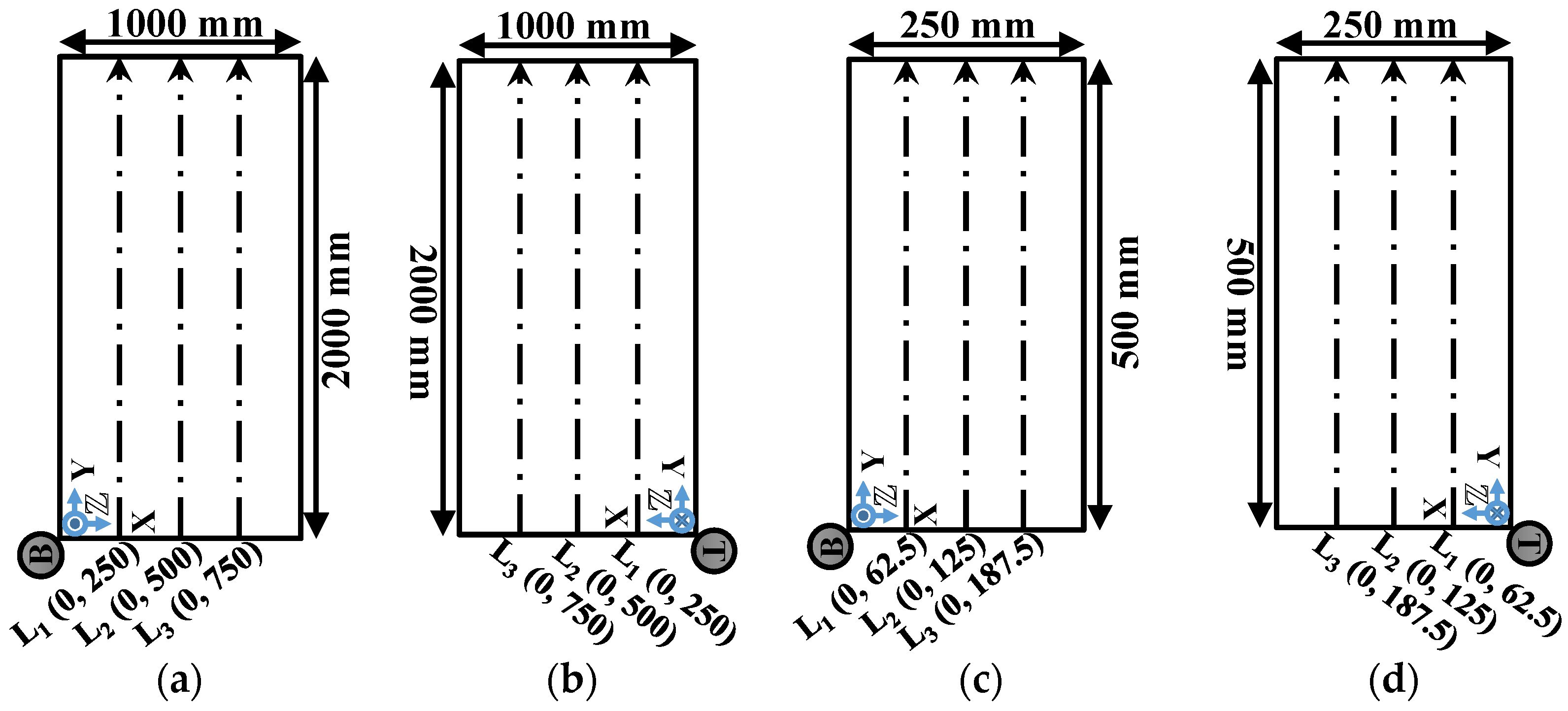
2.3. Surface Roughness Measurements
2.3.1. Roughness Measurements Using the Profilometer
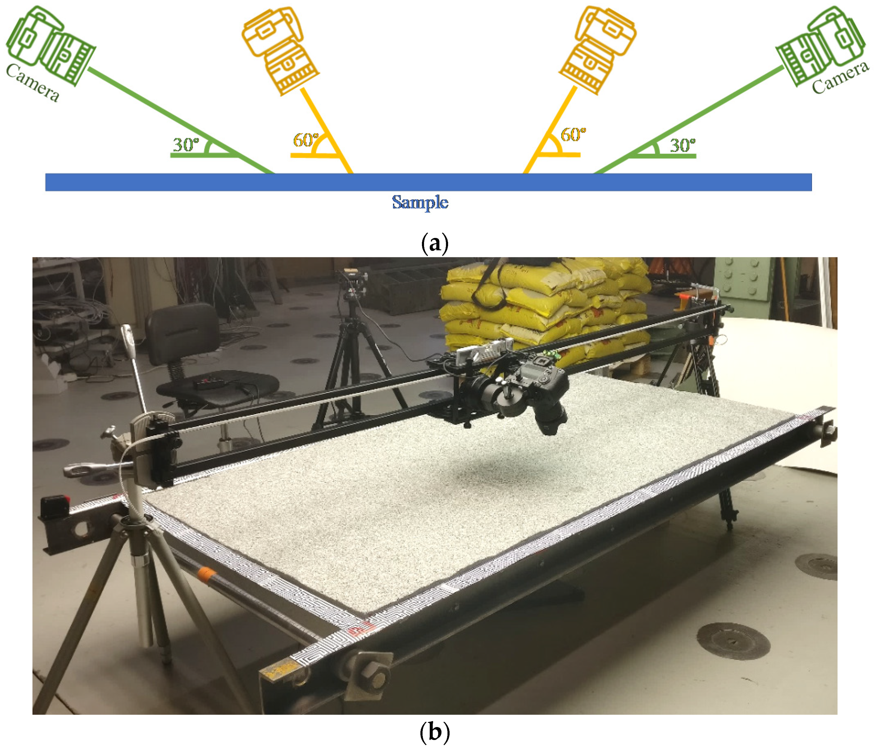
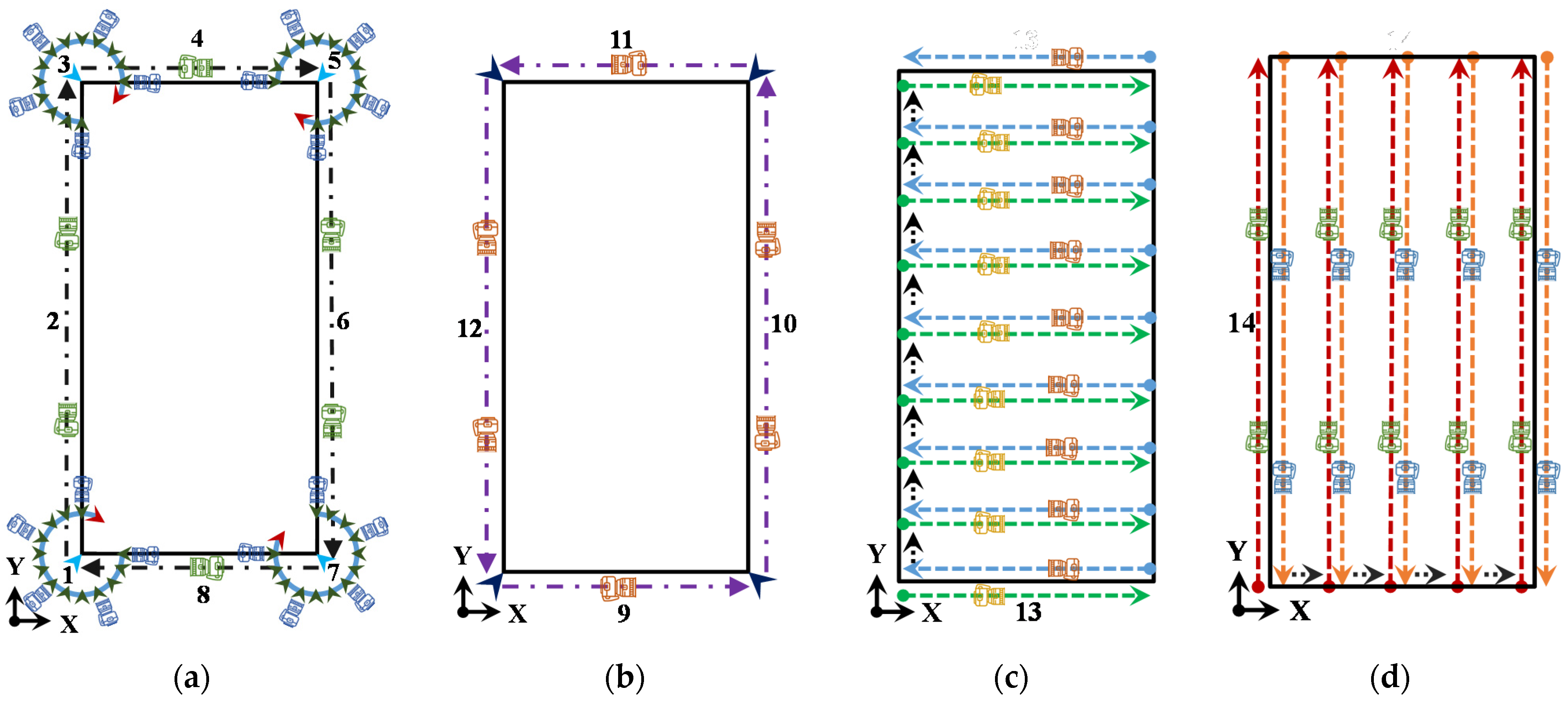
2.3.2. Roughness Measurements Using Photogrammetry
2.4. Photogrammetric Joint Roughness Coefficient (JRC) Calculation from a 2D Line
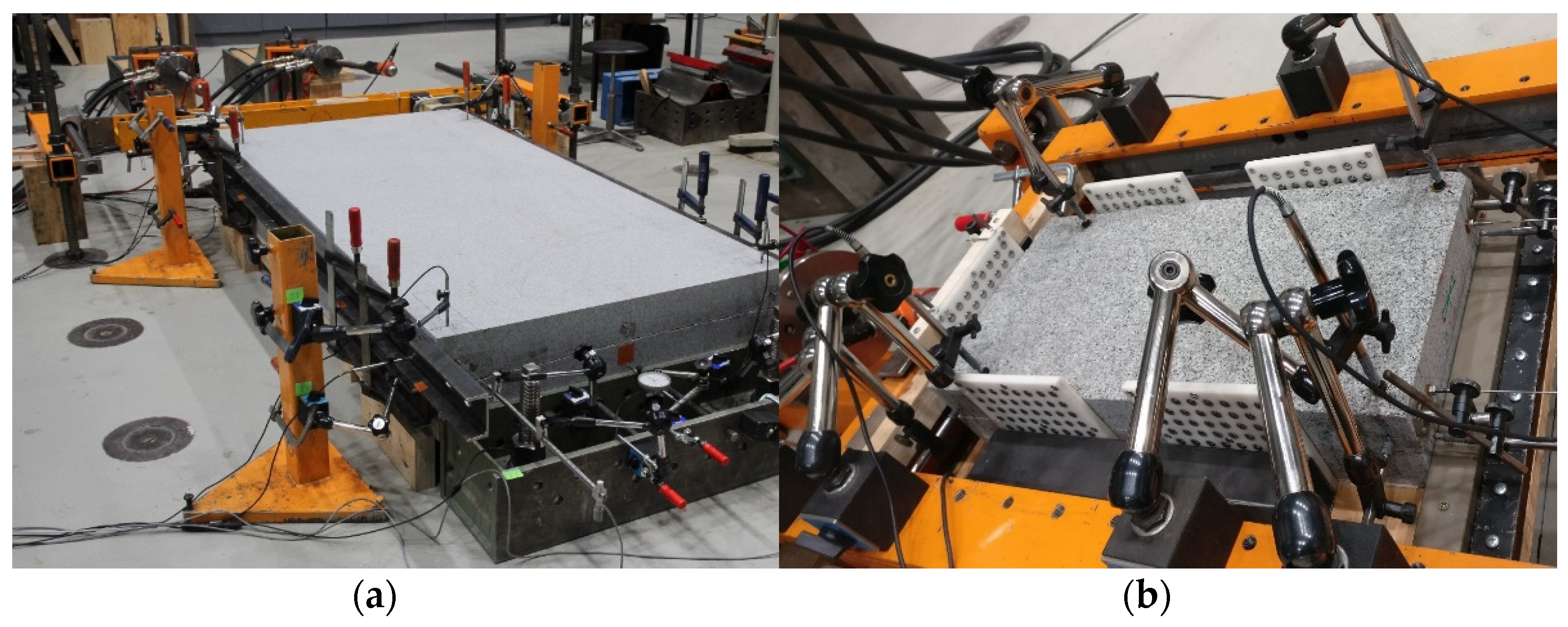
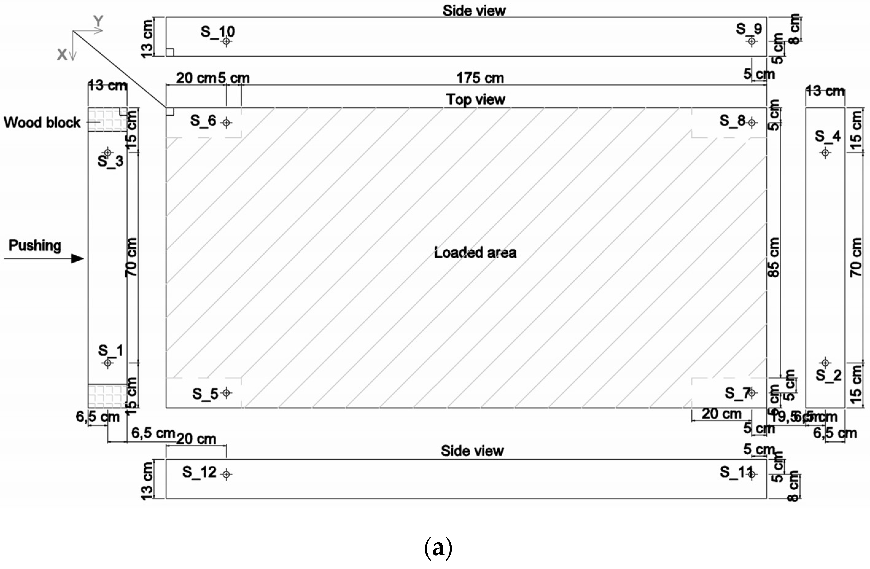
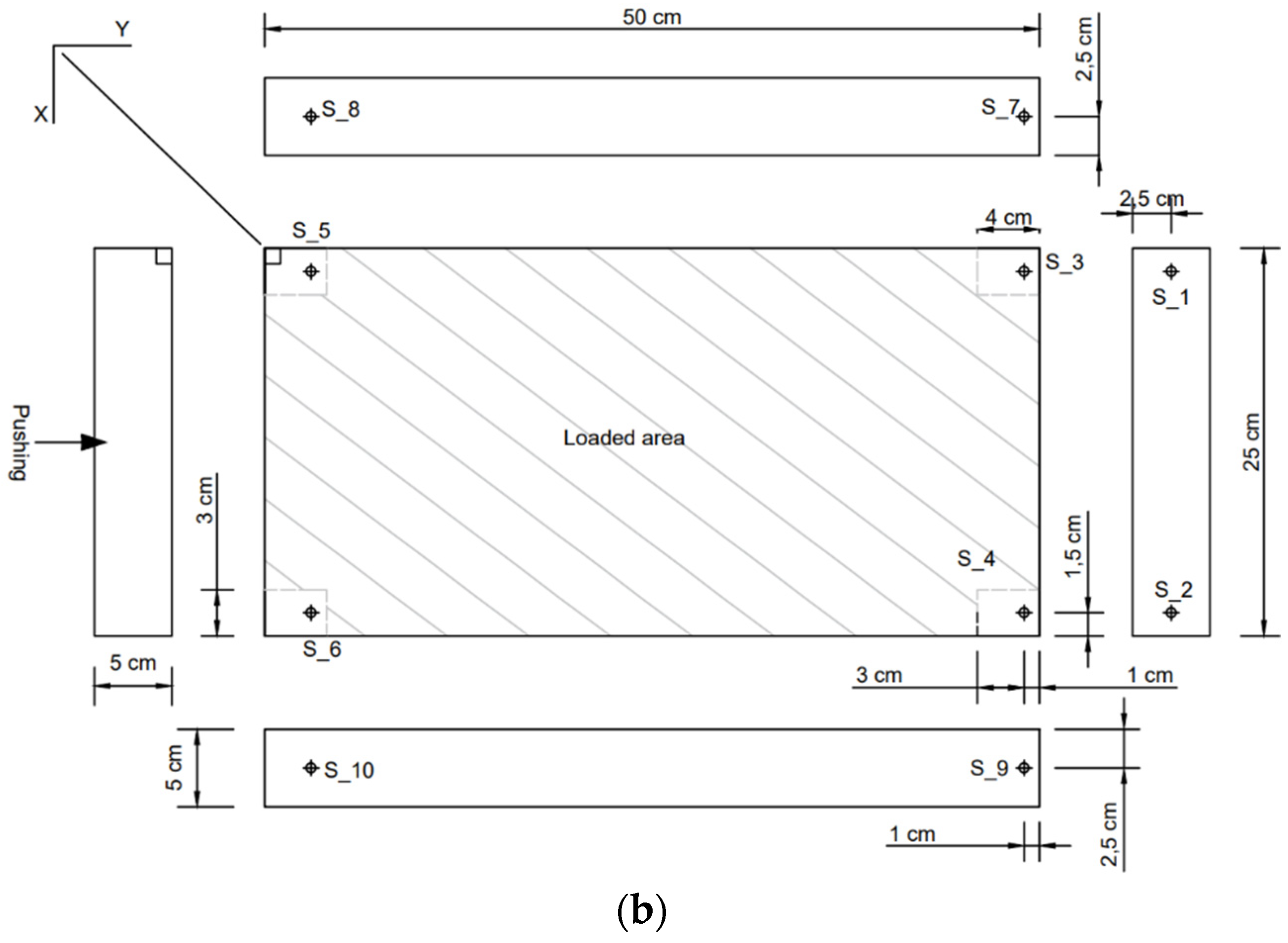
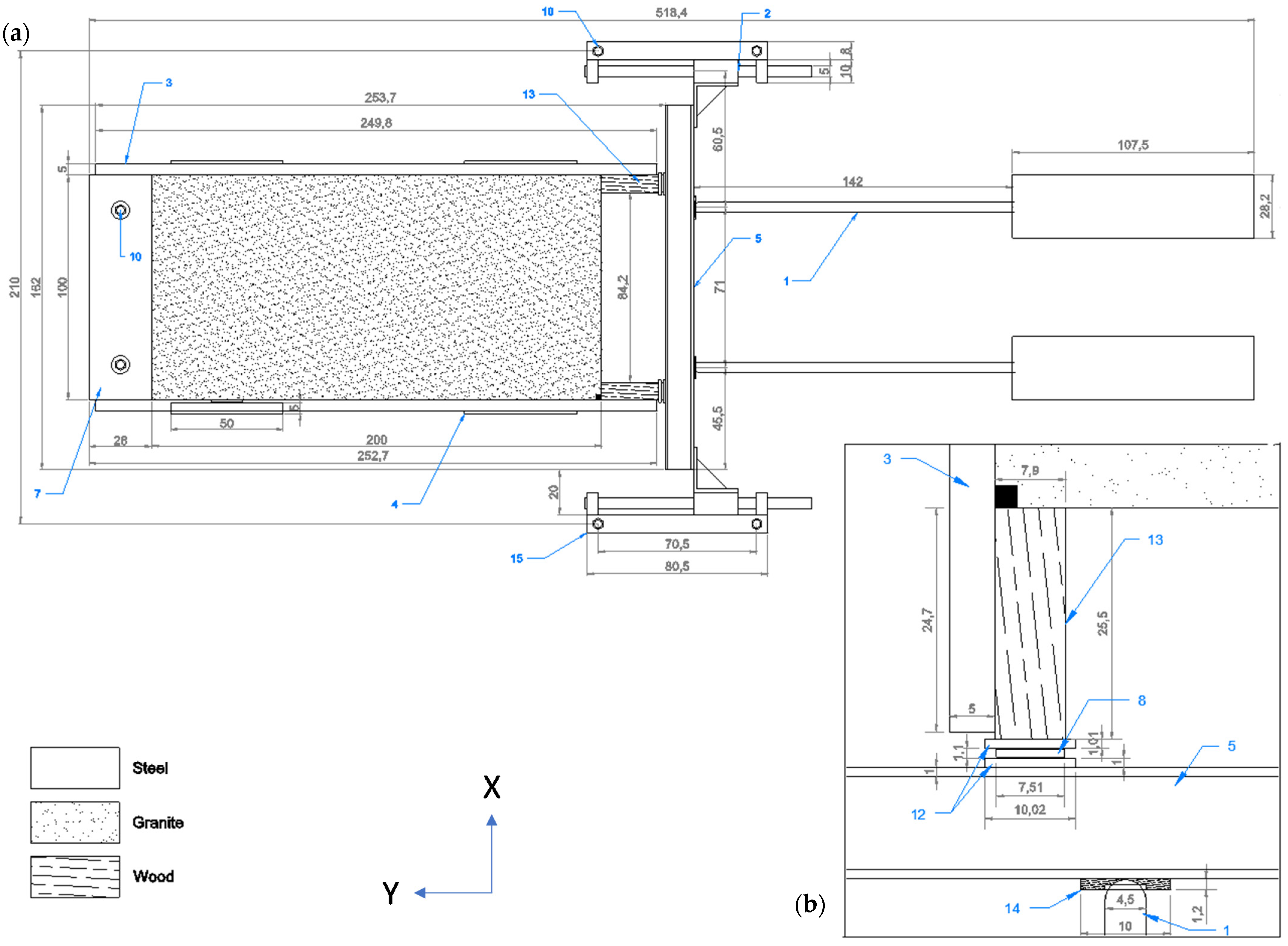
2.5. Push-Shear Test Setup
2.6. Estimation of Peak Friction Angle
3. Results and Discussions
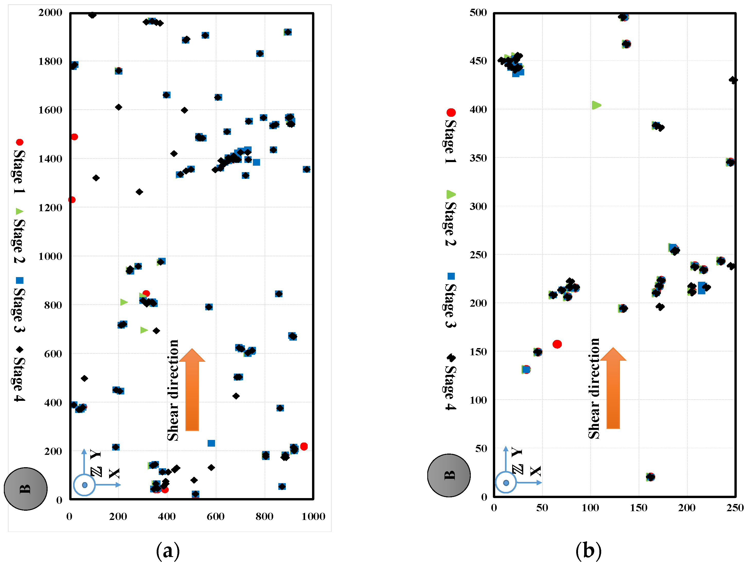
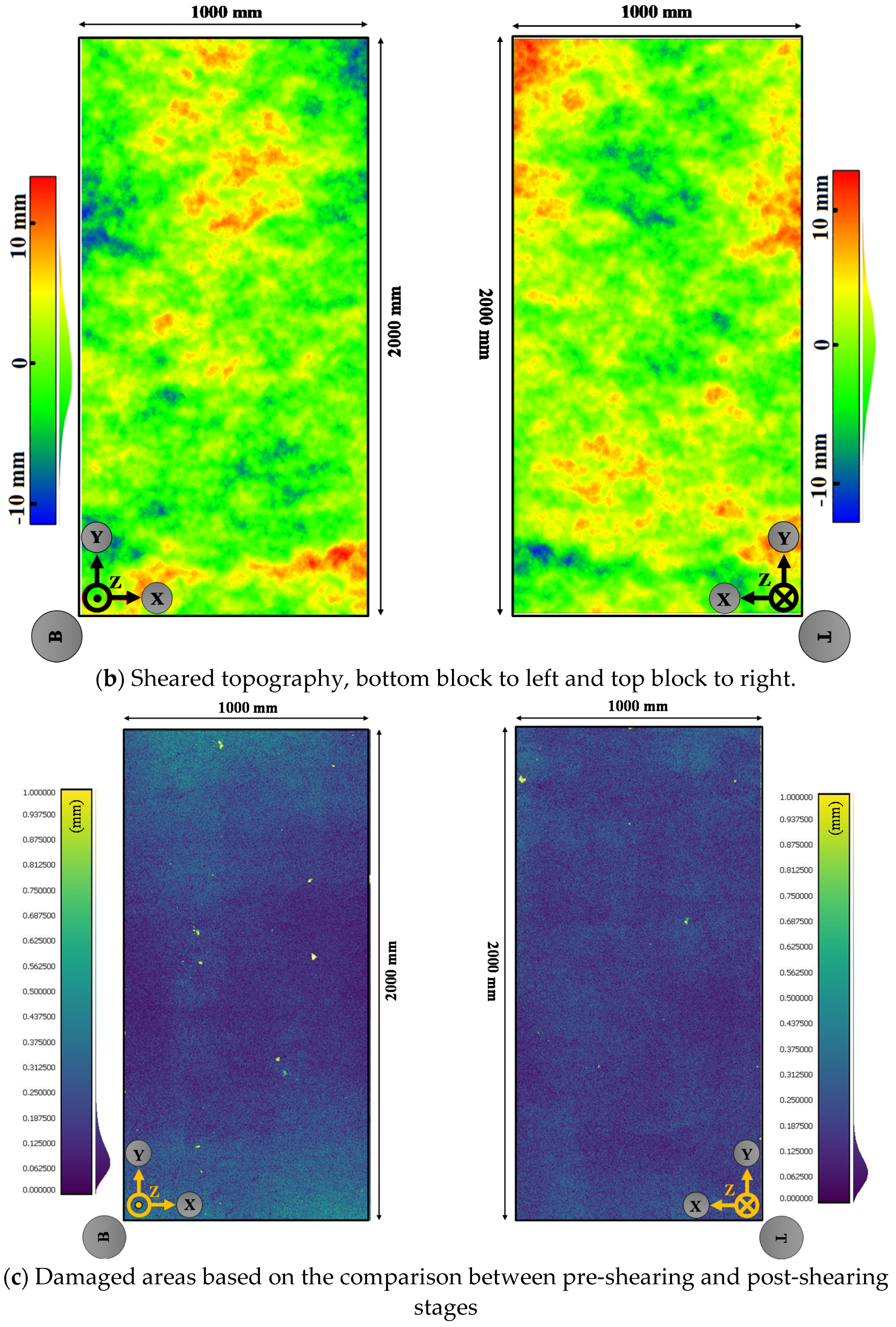
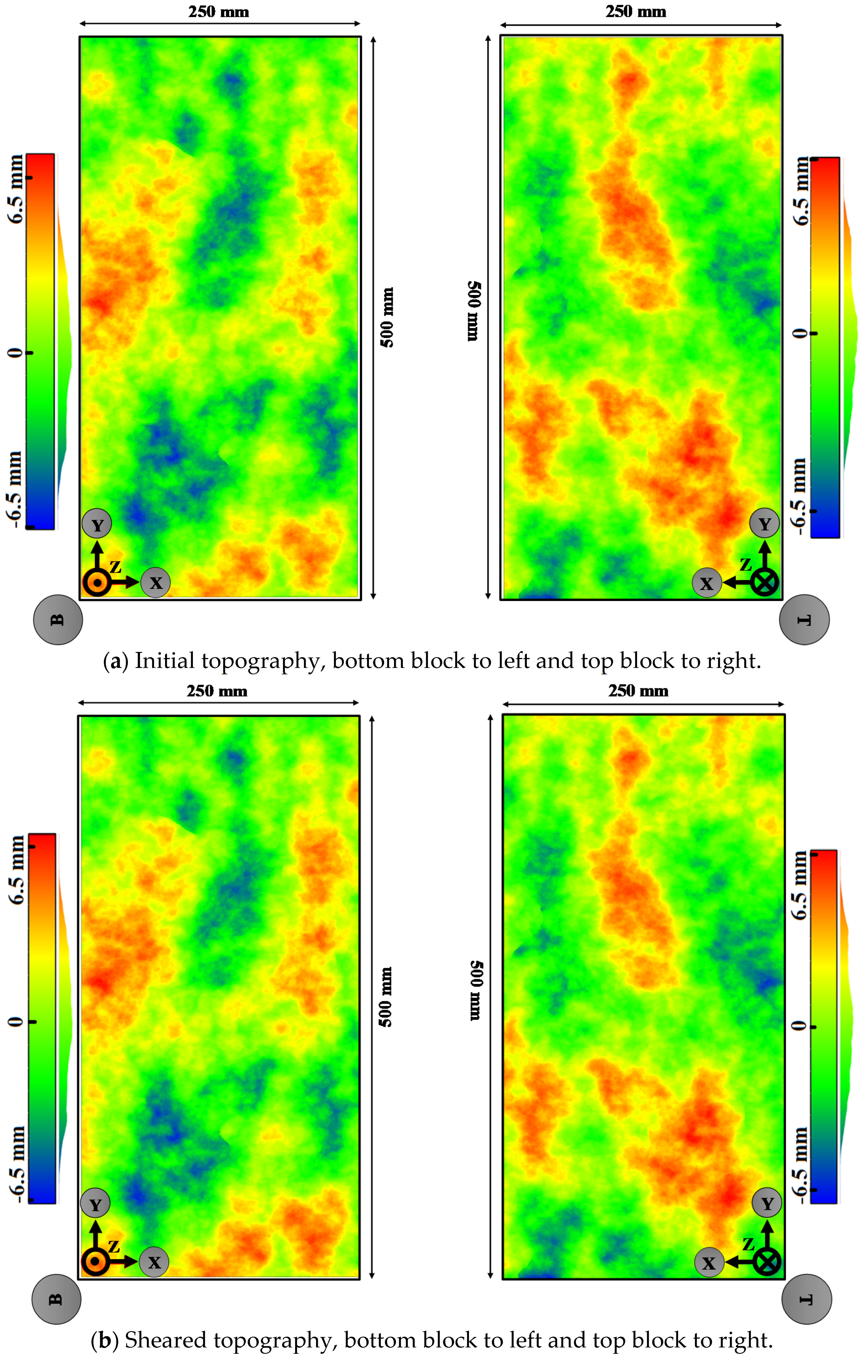
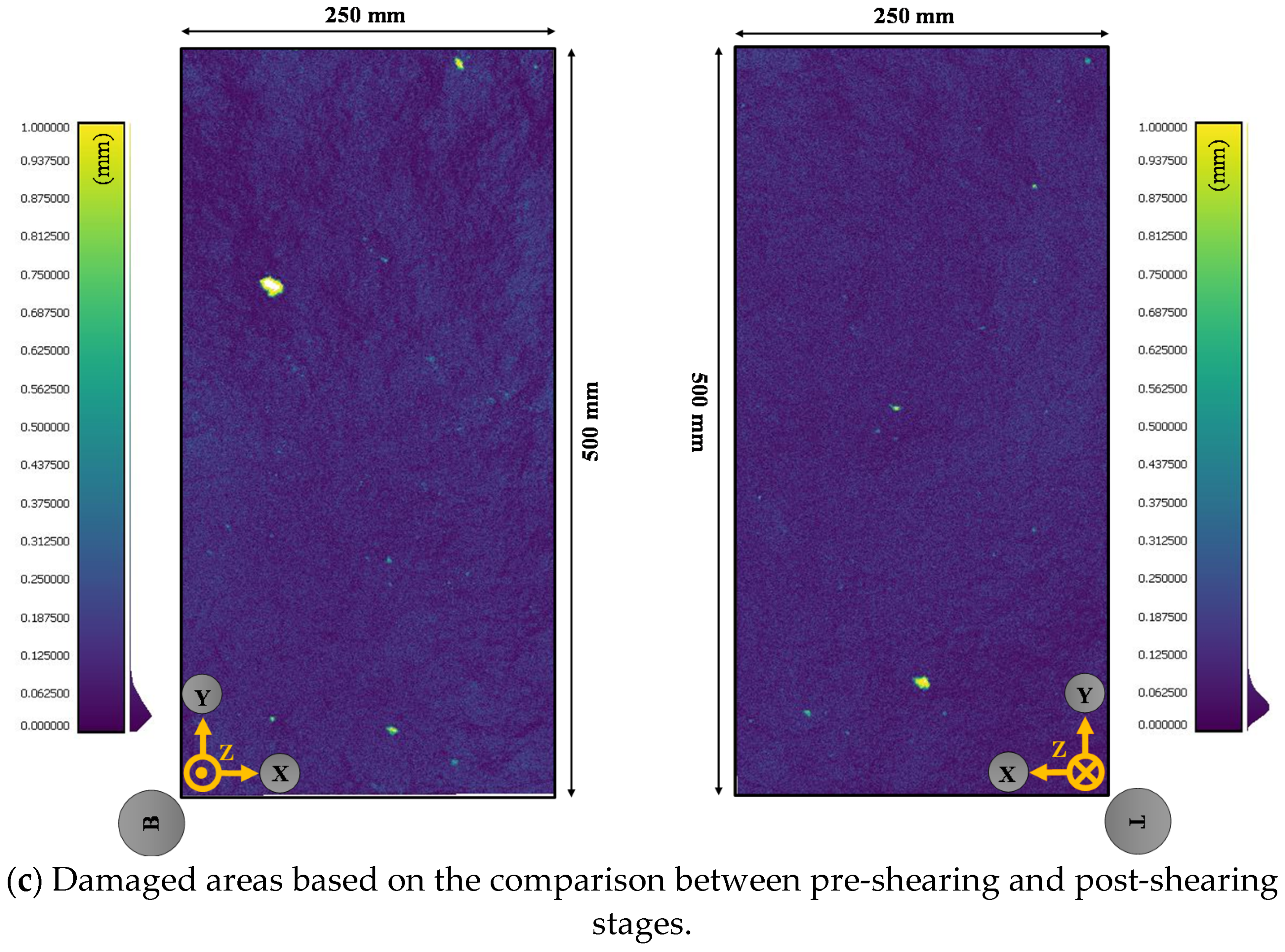
3.1. Characterization of Damaged Areas of the Fracture Surface
3.1.1. JRC Estimated by the Profilometer
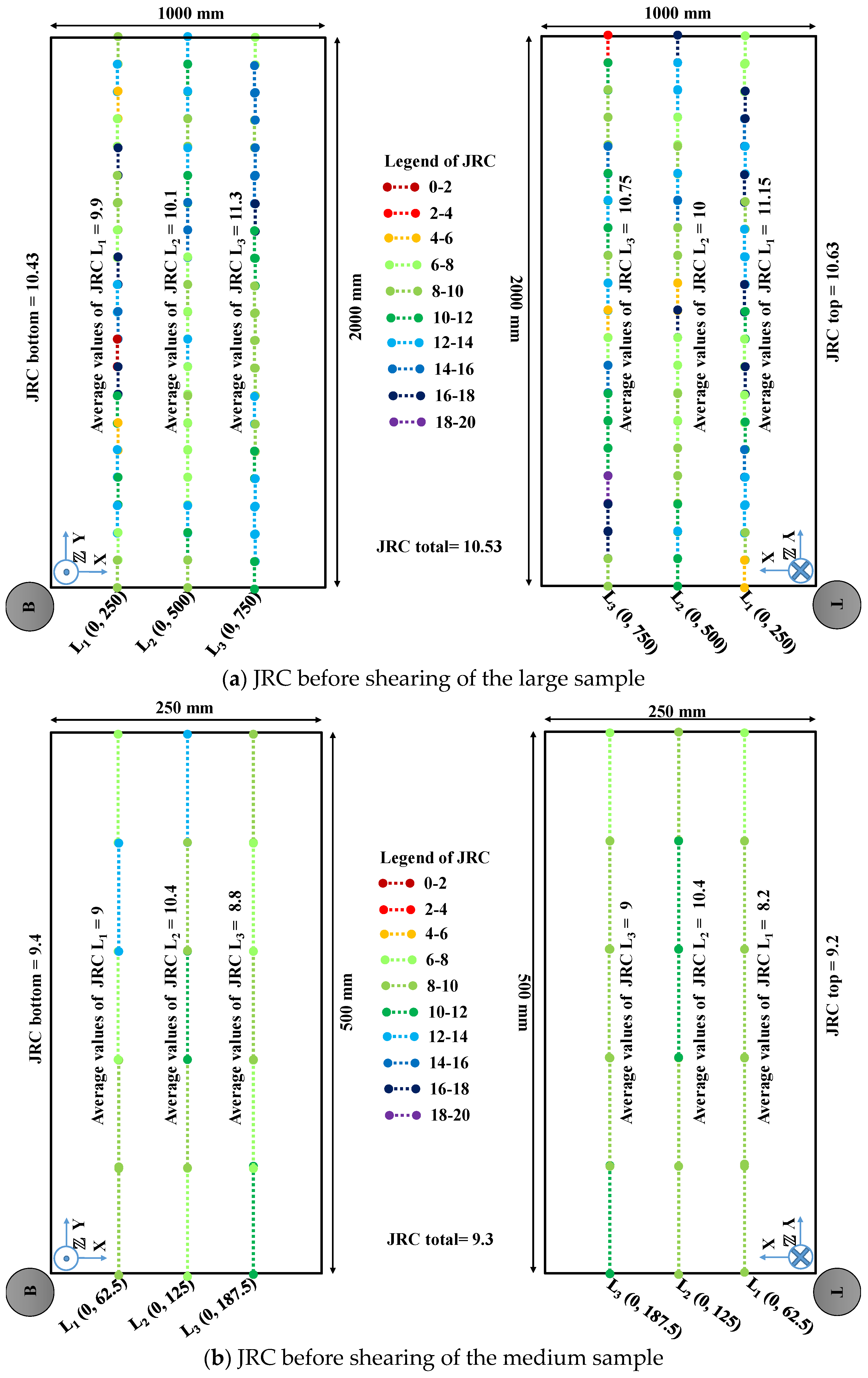
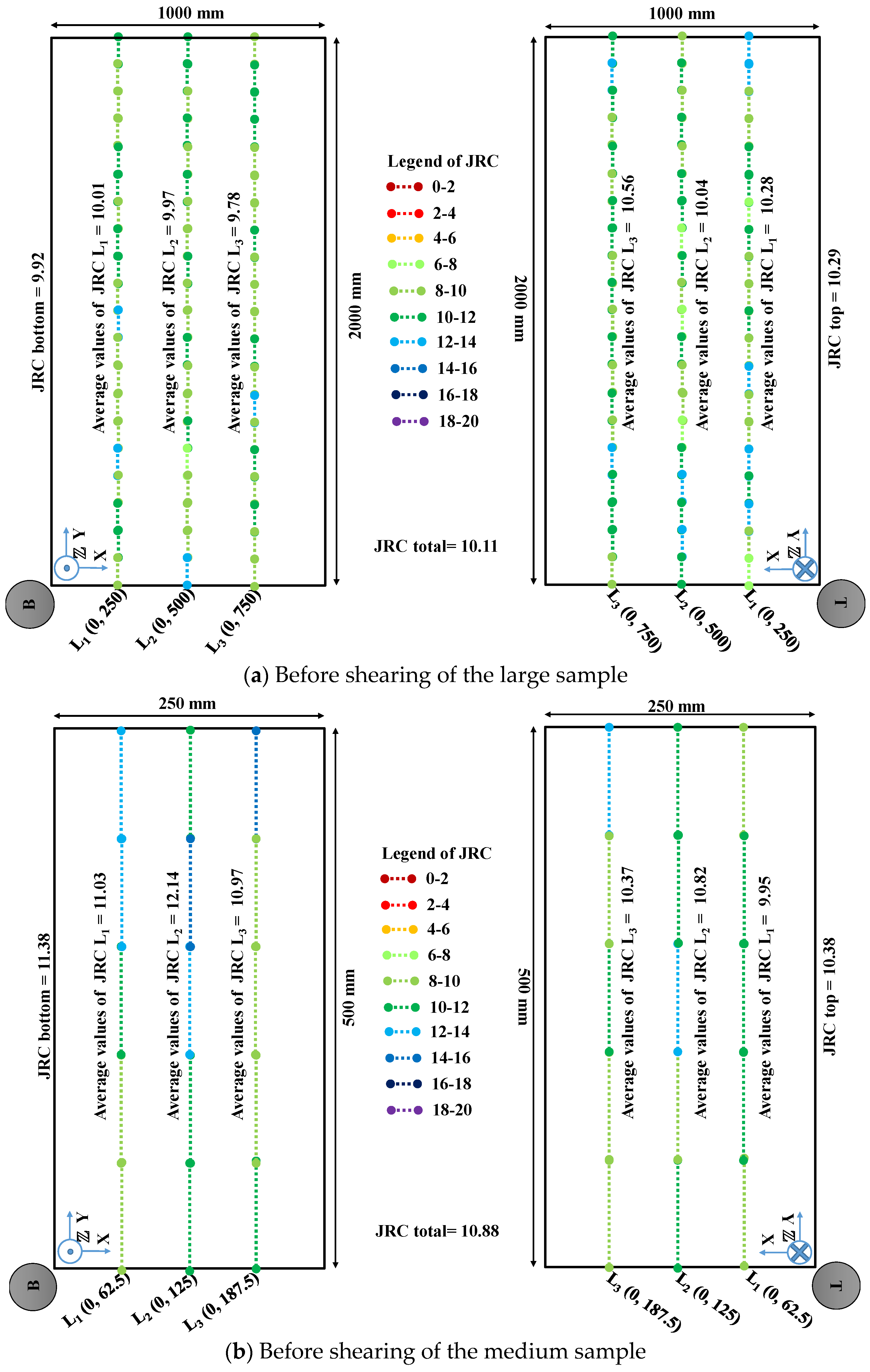
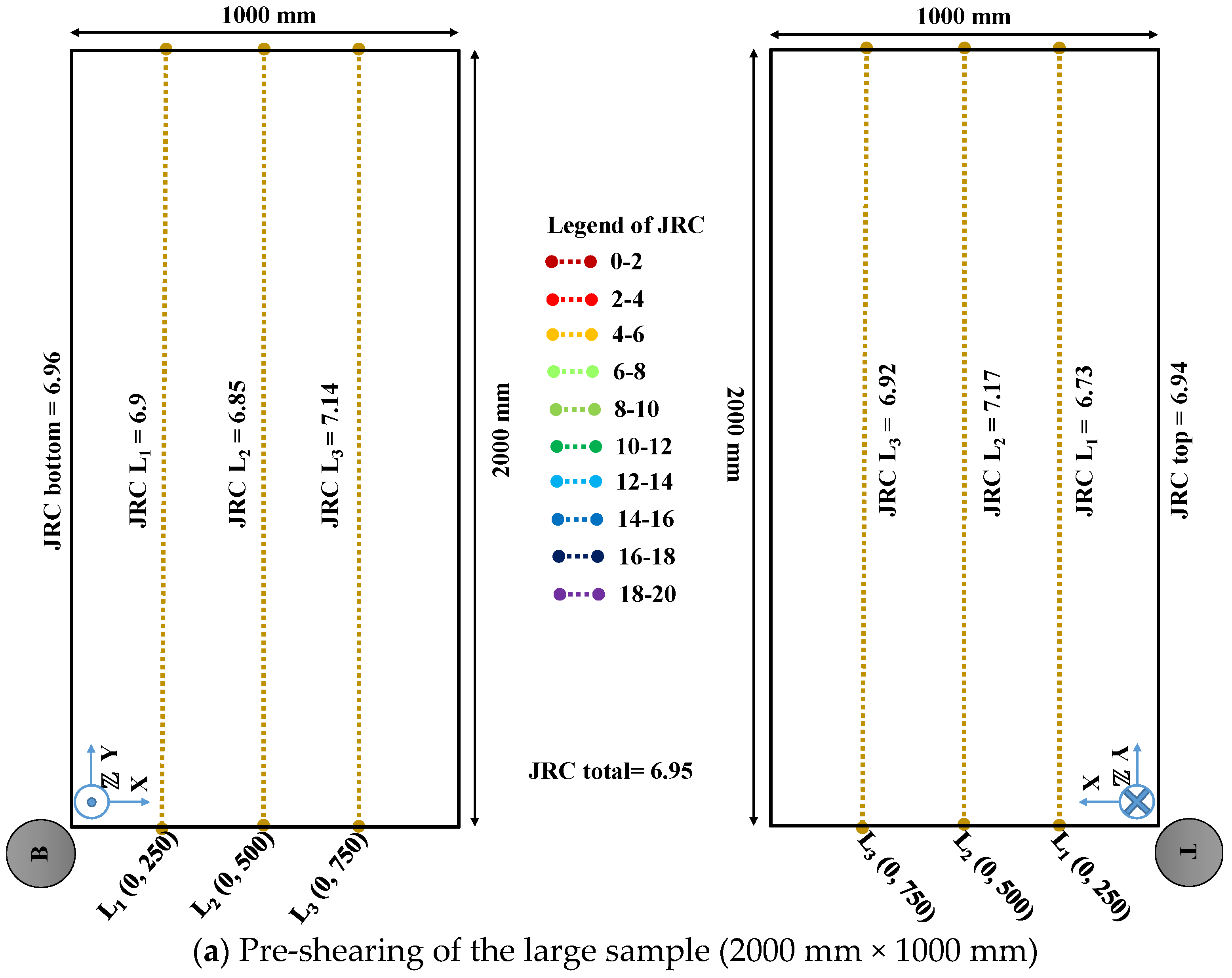
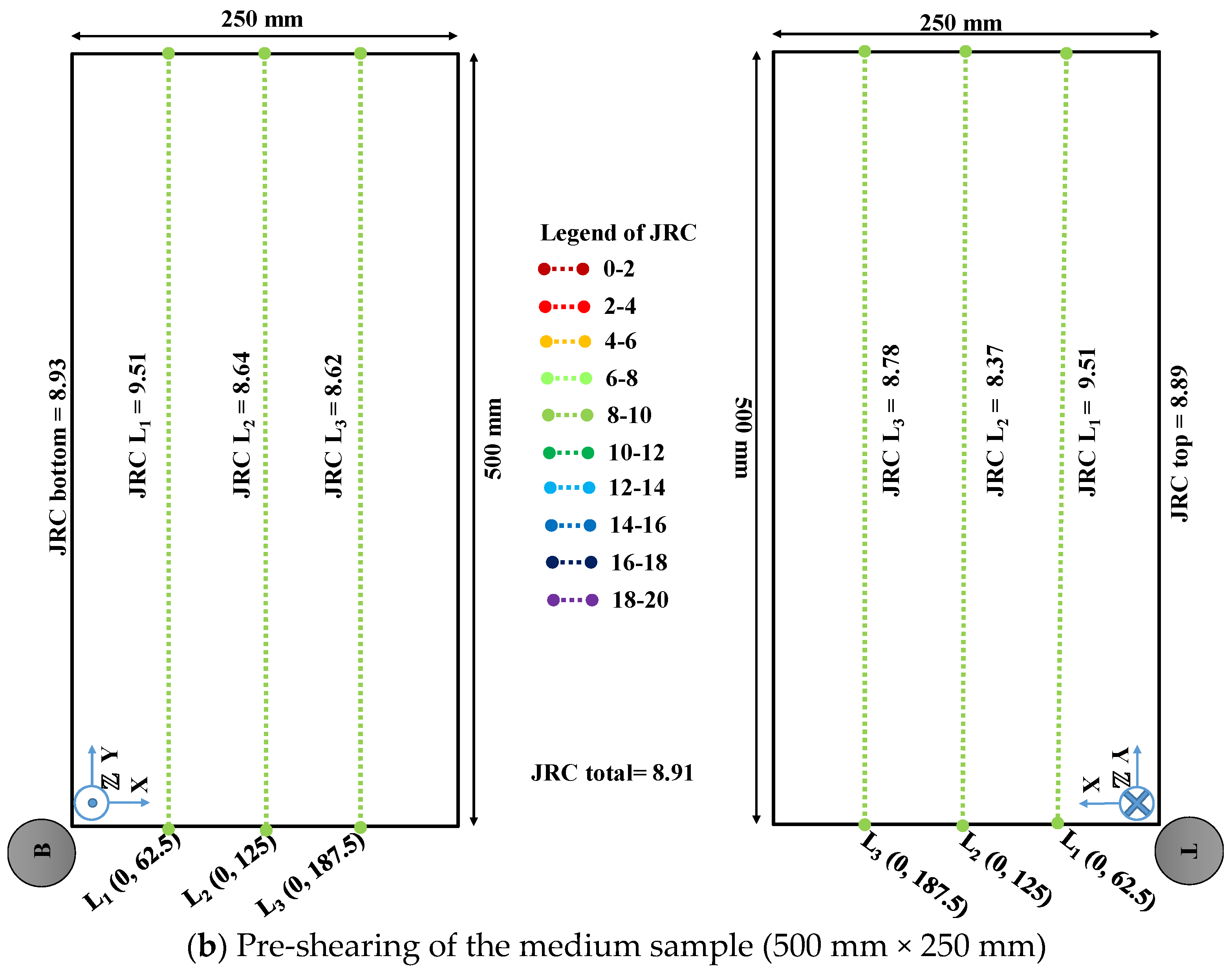
3.1.2. Photogrammetric JRC Values
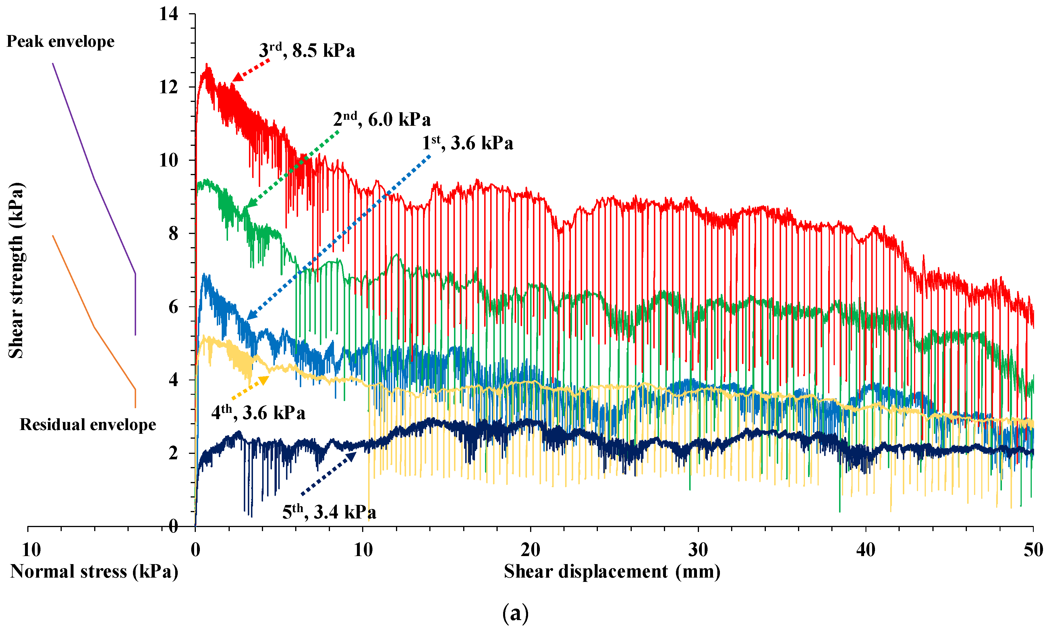
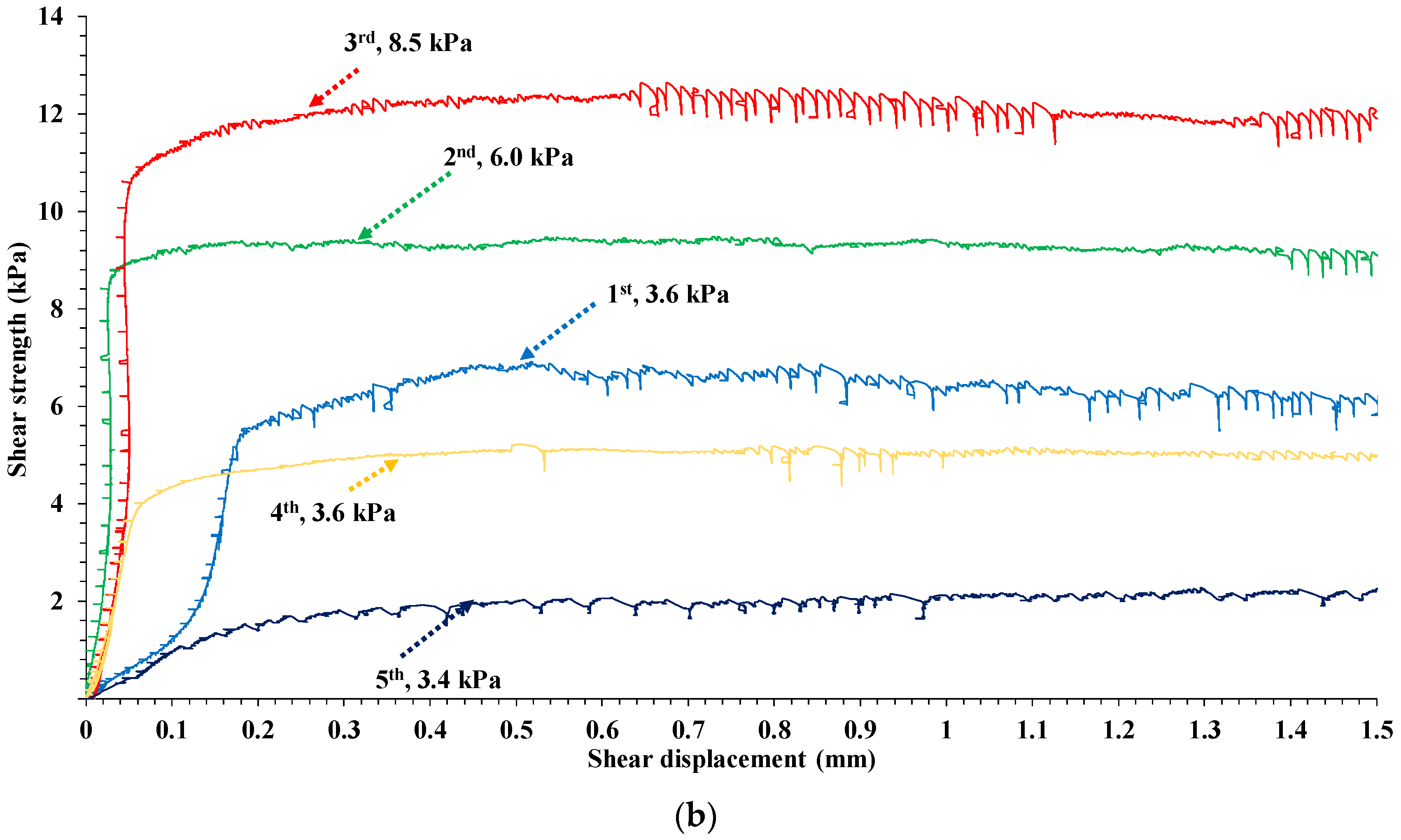
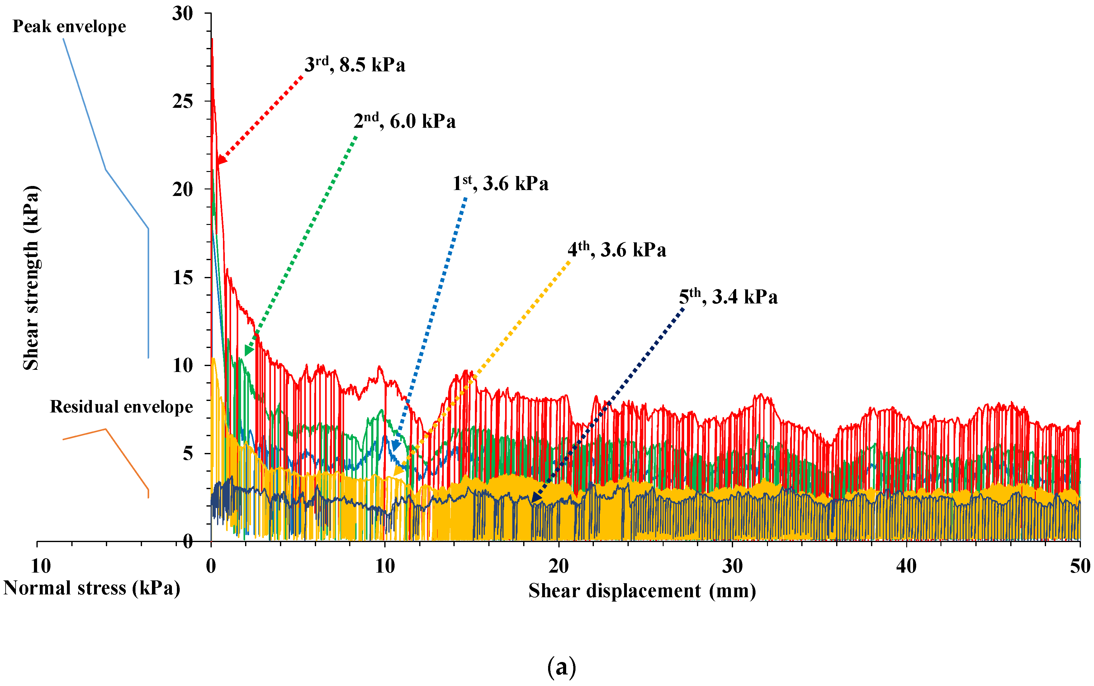
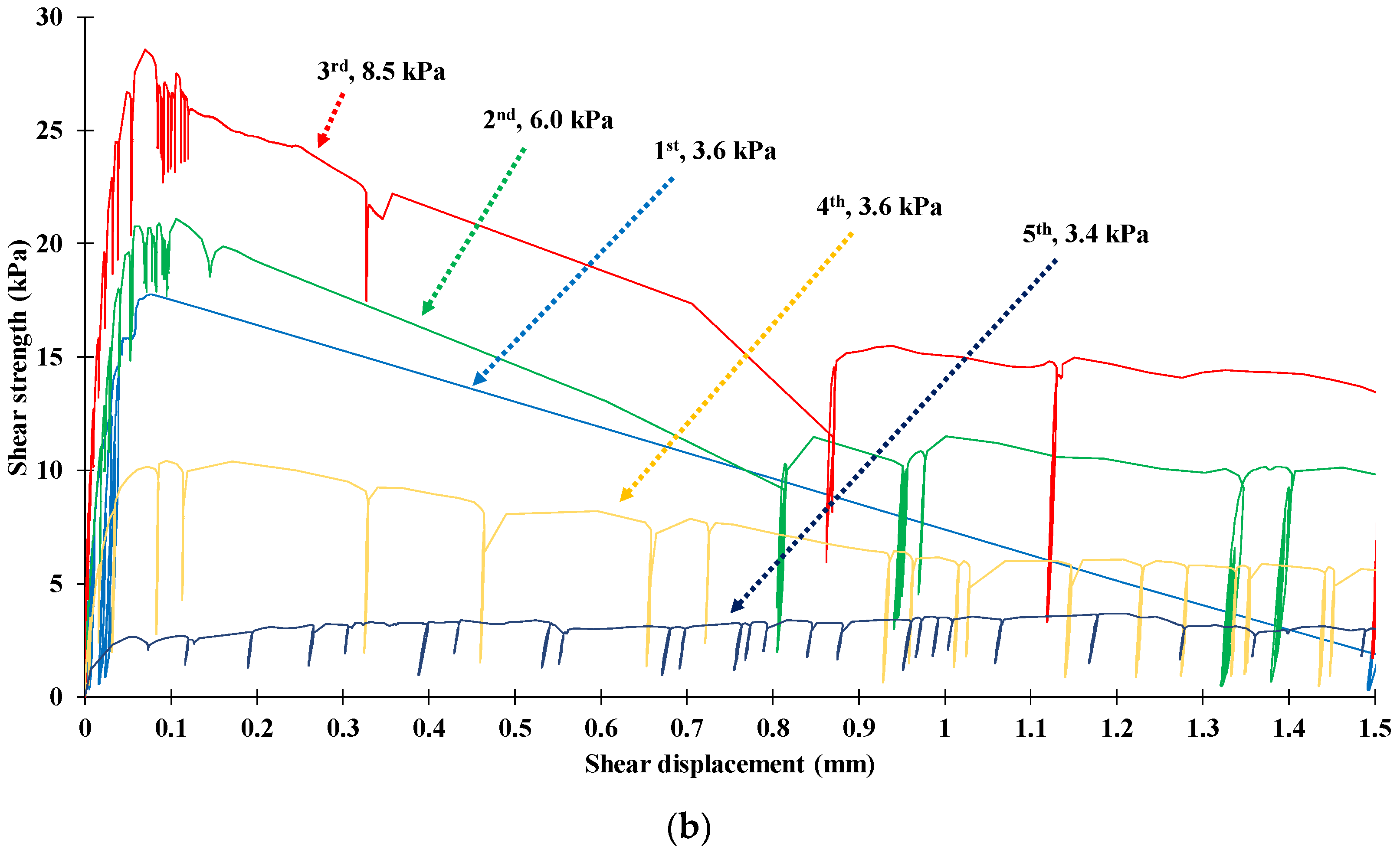
3.2. Shear Test Diagrams
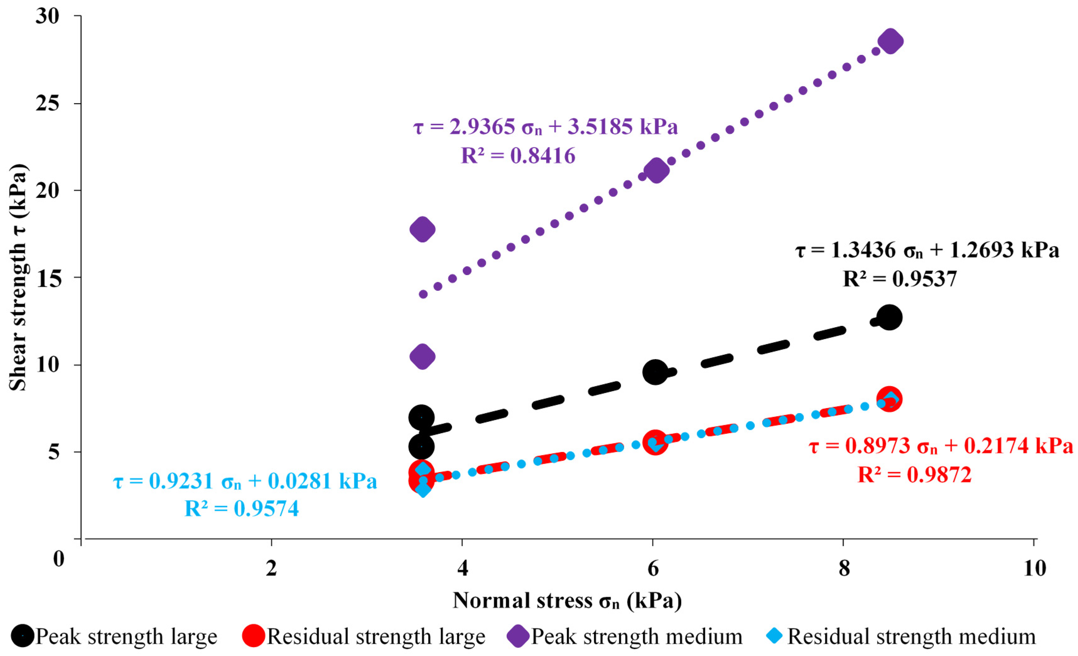
3.3. Method Comparison for Peak Friction Angles
4. Conclusions
Author Contributions
Funding
Acknowledgments
Conflicts of Interest
Appendix A. Experimental


References
- Castelli, M.; Re, F.; Scavia, C.; Zaninett, A. Experimental evaluation of scale effects on the mechanical behavior of rock joints. In Proceedings of the EUROCK 2001 Rock Mechanics—A Challenge for Society, Espoo, Finland, 3–7 June 2001. [Google Scholar]
- Bandis, S. Experimental Studies of Scale Effects on Shear Strength, and Deformation of Rock Joints. Ph.D. Thesis, University of Leeds, Leeds, UK, 1980. [Google Scholar]
- Bandis, S.; Lumsden, A.C.; Barton, N.R. Experimental studies of scale effects on the shear behavior of rock joints. Int. J. Rock Mech. Min. Sci. Geomech. Abstr. 1981, 18, 1–21. [Google Scholar] [CrossRef]
- Patton, F.D. Multiple modes of shear failure in rock. In Proceedings of the 1st ISRM Congress, International Society for Rock Mechanics and Rock Engineering, Lisbon, Portugal, 25 September–1 October 1966. [Google Scholar]
- Barton, N.; Choubey, V. The shear strength of rock joints in theory and practice. Rock Mech. 1977, 10, 1–54. [Google Scholar] [CrossRef]
- Zhao, J. Joint surface matching and shear strength part A: Joint matching coefficient (JMC). Int. J. Rock Mech. Min. Sci. 1997, 34, 173–178. [Google Scholar] [CrossRef]
- Zhao, J. Joint surface matching and shear strength part B: JRC-JMC shear strength criterion. Int. J. Rock Mech. Min. Sci. 1997, 34, 179–185. [Google Scholar] [CrossRef]
- Cruden, D.M.; Hu, X.Q. Basic friction angles of carbonate rocks from Kananaskis country, Canada. Bull. Int. Assoc. Eng. Geol. 1988, 38, 55–59. [Google Scholar] [CrossRef]
- Barton, N. The shear strength of rock and rock joints. Int. J. Rock Mech. Min. Sci. Geomech. Abstr. 1976, 13, 255–279. [Google Scholar] [CrossRef]
- Ulusay, R.; Karakul, H. Assessment of basic friction angles of various rock types from Turkey under dry, wet and submerged conditions and some considerations on tilt testing. Bull. Eng. Geol. Environ. 2016, 75, 1683–1699. [Google Scholar] [CrossRef]
- Özvan, A.; Dinçer, İ.; Acar, A.; Özvan, B. The effects of discontinuity surface roughness on the shear strength of weathered granite joints. Bull. Eng. Geol. Environ. 2014, 73, 801–813. [Google Scholar] [CrossRef]
- Brown, S.R. Fluid flow through rock joints: The effect of surface roughness. J. Geophys. Res. B Solid Earth 1987, 92, 1337–1347. [Google Scholar] [CrossRef]
- Cravero, M.; Iabichino, G.; Piovano, V. Analysis of large joint profiles related to rock slope instabilities. In Proceedings of the 8th ISRM Congress, International Society for Rock Mechanics and Rock Engineering, Tokyo, Japan, 25 September 1995. [Google Scholar]
- Johansson, F. Influence of scale and matedness on the peak shear strength of fresh, unweathered rock joints. Int. J. Rock Mech. Min. Sci. 2016, 82, 36–47. [Google Scholar] [CrossRef] [Green Version]
- Barton, N. Review of a new shear-strength criterion for rock joints. Eng. Geol. 1973, 7, 287–332. [Google Scholar] [CrossRef]
- Serasa, A.S.; Lai, G.T.; Rafek, A.G.; Hussin, A. Peak friction angle estimation from joint roughness coefficient of discontinuities of limestone in Peninsular Malaysia. Sains Malays. 2017, 46, 181–188. [Google Scholar] [CrossRef]
- Rafek, A.G.; Lai, G.T.; Serasa, A.S. A Low Cost Alternative Approach to Geological Discontinuity Roughness Quantification. In IAEG/AEG Annual Meeting Proceedings, San Francisco, California; Springer: Cham, Switzerland, 2019. [Google Scholar]
- Tse, R.; Cruden, D.M. Estimating joint roughness coefficients. Int. J. Rock Mech. Min. Sci. Geomech. Abstr. 1979, 16, 303–307. [Google Scholar] [CrossRef]
- Maerz, N.H.; Franklin, J.A.; Bennett, C.P. Joint roughness measurement using shadow profilometry. Int. J. Rock Mech. Min. Sci. Geomech. Abstr. 1990, 27, 329–343. [Google Scholar] [CrossRef]
- Tatone, B.S.; Grasselli, G. A new 2D discontinuity roughness parameter and its correlation with JRC. Int. J. Rock Mech. Min. Sci. 2010, 47, 1391–1400. [Google Scholar] [CrossRef]
- Zhang, G.; Karakus, M.; Tang, H.; Ge, Y.; Zhang, L. A new method estimating the 2D joint roughness coefficient for discontinuity surfaces in rock masses. Int. J. Rock Mech. Min. Sci. 2014, 72, 191–198. [Google Scholar] [CrossRef]
- Magsipoc, E.; Zhao, Q.; Grasselli, G. 2D and 3D Roughness Characterization. Rock Mech. Rock Eng. 2020, 53, 1495–1519. [Google Scholar] [CrossRef]
- Brown, S.R.; Scholz, C.H. Broad bandwidth study of the topography of natural rock surfaces. J. Geophys. Res. B Solid Earth 1985, 90, 12575–12582. [Google Scholar] [CrossRef]
- Thom, C.A.; Brodsky, E.E.; Carpick, R.W.; Pharr, G.M.; Oliver, W.C.; Goldsby, D.L. Nanoscale roughness of natural fault surfaces controlled by scale-dependent yield strength. Geophys. Res. Lett. 2017, 44, 9299–9307. [Google Scholar] [CrossRef]
- Lanaro, F. A random field model for surface roughness and aperture of rock fractures. Int. J. Rock Mech. Min. Sci. 2000, 37, 1195–1210. [Google Scholar] [CrossRef]
- Ficker, T.; Martišek, D. Digital fracture surfaces and their roughness analysis: Applications to cement-based materials. Cem. Concr. Res. 2012, 42, 827–833. [Google Scholar] [CrossRef]
- Renard, F.; Mair, K.; Gundersen, O. Surface roughness evolution on experimentally simulated faults. J. Struct. Geol. 2012, 45, 101–112. [Google Scholar] [CrossRef]
- Mah, J.; Samson, C.; McKinnon, S.D.; Thibodeau, D. 3D laser imaging for surface roughness analysis. Int. J. Rock Mech. Min. Sci. 2013, 58, 111–117. [Google Scholar] [CrossRef]
- Fardin, N.; Feng, Q.; Stephansson, O. Application of a new in situ 3D laser scanner to study the scale effect on the rock joint surface roughness. Int. J. Rock Mech. Min. Sci. 2004, 41, 329–335. [Google Scholar] [CrossRef]
- Sagy, A.; Brodsky, E.E.; Axen, G.J. Evolution of fault-surface roughness with slip. Geology 2007, 35, 283–286. [Google Scholar] [CrossRef]
- Grasselli, G.; Wirth, J.; Egger, P. Quantitative three-dimensional description of a rough surface and parameter evolution with shearing. Int. J. Rock Mech. Min. Sci. 2002, 39, 789–800. [Google Scholar] [CrossRef]
- Tatone, B.S. Quantitative Characterization of Natural Rock Discontinuity Roughness In-Situ and in the Laboratory. Ph.D. Thesis, University of Toronto, Toronto, ON, Canada, 2009. [Google Scholar]
- Tatone, B.S.; Grasselli, G. Use of a stereo-topometric measurement system for the characterization of rock joint roughness in-situ and in the laboratory. Rock Engineering in Difficult Conditions. In Proceedings of the 3rd CANUS Rock Mechanics Symposium, Toronto, ON, Canada, 9−15 May 2009. [Google Scholar]
- El-Soudani, S.M. Profilometric analysis of fractures. Metallography 1978, 11, 247–336. [Google Scholar] [CrossRef]
- Unal, M.; Yakar, M.; Yildiz, F. Discontinuity surface roughness measurement techniques and the evaluation of digital photogrammetric method. In Proceedings of the 20th international Congress for Photogrammetry and Remote Sensing (ISPRS), Istanbul, Turkey, 12−23 July 2004; pp. 1103–1108. [Google Scholar]
- Lee, H.S.; Ahn, K.W. A prototype of digital photogrammetric algorithm for estimating roughness of rock surface. Geosci. J. 2004, 8, 333–341. [Google Scholar] [CrossRef]
- Haneberg, W.C. Directional roughness profiles from three-dimensional photogrammetric or laser scanner point clouds. In Proceedings of the 1st Canada-US Rock Mechanics Symposium, Vancouver, BC, Canada, 27 May 2007. [Google Scholar]
- Baker, B.R.; Gessner, K.; Holden, E.J.; Squelch, A.P. Automatic detection of anisotropic features on rock surfaces. Geosphere 2008, 4, 418–428. [Google Scholar] [CrossRef]
- Poropat, G.V. Remote characterisation of surface roughness of rock discontinuities. In First Southern Hemisphere International Rock Mechanics Symposium; Potvin, Y., Carter, J., Dyskin, A., Jeffrey, R., Eds.; Australian Centre for Geomechanics: Perth, Australia, 2008; pp. 447–458. [Google Scholar] [CrossRef]
- Poropat, G.V. Measurement of surface roughness of rock discontinuities. In Proceedings of the 3rd CANUS Rock Mechanics Symposium, Toronto, ON, Canada, 9−15 May 2009. [Google Scholar]
- Nilsson, M.; Edelbro, C.; Sharrock, G. Small scale joint surface roughness evaluation using digital photogrammetry. In Proceedings of the ISRM International Symposium-EUROCK 2012, Stockholm, Sweden, 28 May 2012. [Google Scholar]
- Kim, D.H.; Gratchev, I.; Balasubramaniam, A. Determination of joint roughness coefficient (JRC) for slope stability analysis: A case study from the Gold Coast area, Australia. Landslides 2013, 10, 657–664. [Google Scholar] [CrossRef] [Green Version]
- Kim, D.H.; Gratchev, I.; Poropat, G.V. The determination of joint roughness coefficient using three-dimensional models for slope stability analysis. In 2013 International Symposium on Slope Stability in Open Pit Mining and Civil Engineering; Australian Centre for Geomechanics: Perth, Australia, 2013; pp. 281–289. [Google Scholar] [CrossRef] [Green Version]
- Kim, D.H.; Poropat, G.V.; Gratchev, I.; Balasubramaniam, A. Improvement of photogrammetric JRC data distributions based on parabolic error models. Int. J. Rock Mech. Min. Sci. 2015, 80, 19–30. [Google Scholar] [CrossRef]
- Kim, D.H.; Poropat, G.; Gratchev, I.; Balasubramaniam, A. Assessment of the accuracy of close distance photogrammetric JRC data. Rock Mech. Rock Eng. 2016, 49, 4285–4301. [Google Scholar] [CrossRef] [Green Version]
- Sirkiä, J.; Kallio, P.; Iakovlev, D.; Uotinen, L. Photogrammetric calculation of JRC for rock slope support design. In Eighth International Symposium on Ground Support in Mining and Underground Construction; Nordlund, E., Jones, T.H., Eitzenberger, A., Eds.; Ground Support: Luleå, Sweden, 2016. [Google Scholar]
- Iakovlev, D.; Sirkiä, J.; Kallio, P.; Uotinen, L. Determination of joint mechanical parameters for stability analysis in low stress open pit mines. In Proceedings of the 7th International Symposium on In-Situ Rock Stress, Tampere, Finland, 10–12 May 2016; Johansson, E., Raasakka, V., Eds.; Suomen Rakennusinsinöörien Liitto: Tampere, Finland, 2016. [Google Scholar]
- Dzugala, M. Pull Experiment to Validate the Photogrammetrically Predicted Friction Angle of Rock Discontinuities. Master’s Thesis, Aalto University, Espoo, Finland, 2016. [Google Scholar]
- Dzugala, M.; Sirkiä, J.; Uotinen, L.; Rinne, M. Pull experiment to validate photogrammetrically predicted friction angle of rock discontinuities. Procedia Eng. 2017, 191, 378–385. [Google Scholar] [CrossRef]
- Kim, D.H.; Lee, C.H.; Balasubramaniam, A.; Gratchev, I. Application of data mining technique to complement photogrammetric roughness data. In Proceedings of the 20th SEAGC—3rd AGSSEA Conference in conjunction with 22nd Annual Indonesian National Conference on Geotechnical Engineering, Jakarta, Indonesia, 6–7 November 2018. [Google Scholar]
- Bizjak, K.F.; Geršak, A. Quantified joint surface description and joint shear strength of small rock samples. Geologija 2018, 61, 25–32. [Google Scholar] [CrossRef]
- Pitts, A.D.; Salama, A.; Volatili, T.; Giorgioni, M.; Tondi, E. Analysis of fracture roughness control on permeability using sfm and fluid flow simulations: Implications for carbonate reservoir characterization. Geofluids 2019, 2019, 4132386. [Google Scholar] [CrossRef] [Green Version]
- Uotinen, L.; Janiszewski, M.; Baghbanan, A.; Caballero Hernandez, E.; Oraskari, J.; Munukka, H.; Szydlowska, M.; Rinne, M. Photogrammetry for recording rock surface geometry and fracture characterization. In Proceedings of the ISRM International Congress on Rock Mechanics and Rock Engineering, Foz do Iguaçu, Brazil, 13–18 September 2019; CRC Press: Iguassu Falls, Brazil, 2019. [Google Scholar]
- Uotinen, L. Prediction of Stress-Driven Rock Mass Damage in Spent Nuclear Fuel Repositories in Hard Crystalline Rock and in Deep Underground Mines. Ph.D. Thesis, Aalto University, Espoo, Finland, 2018. [Google Scholar]
- Fardin, N.; Stephansson, O.; Jing, L. The scale dependence of rock joint surface roughness. Int. J. Rock Mech. Min. Sci. 2001, 38, 659–669. [Google Scholar] [CrossRef]
- Tatone, B.S.; Grasselli, G. An investigation of discontinuity roughness scale dependency using high-resolution surface measurements. Rock Mech. Rock Eng. 2013, 46, 657–681. [Google Scholar] [CrossRef]
- Bahaaddini, M.; Hagan, P.C.; Mitra, R.; Hebblewhite, B.K. Scale effect on the shear behavior of rock joints based on a numerical study. Eng. Geol. 2014, 181, 212–223. [Google Scholar] [CrossRef]
- Johansson, F.; Stille, H. A conceptual model for the peak shear strength of fresh and unweathered rock joints. Int. J. Rock Mech. Min. Sci. 2014, 69, 31–38. [Google Scholar] [CrossRef]
- Bost, M.; Mouzannar, H.; Rojat, F.; Coubard, G.; Rajot, J.P. Metric Scale Study of the Bonded Concrete-Rock Interface Shear Behavior. KSCE J. Civ. Eng. 2019, 24, 390–403. [Google Scholar] [CrossRef]
- Azinfar, M.J.; Ghazvinian, A.H.; Nejati, H.R. Assessment of scale effect on 3D roughness parameters of fracture surfaces. Eur. J. Environ. Civ. Eng. 2019, 23, 1–28. [Google Scholar] [CrossRef]
- Wang, S.; Masoumi, H.; Oh, J.; Zhang, S. Scale-Size and Structural Effects of Rock Materials; Woodhead Publishing: Sawston, UK, 2020. [Google Scholar]
- Swan, G.; Zongqi, S. Prediction of shear behavior of joints using profiles. Rock Mech. Rock Eng. 1985, 18, 183–212. [Google Scholar] [CrossRef]
- Rasilainen, K. The Finnish Research Programme on Nuclear Waste Management (KYT) 2002–2005. VTT Technical Research Centre of Finland. 2006. Available online: http://www.vtt.fi/inf/pdf/tiedotteet/2006/T2337.pdf (accessed on 27 March 2021).
- Uotinen, L.; Torkan, M.; Janiszewski, M.; Baghbanan, A.; Nieminen, V.; Rinne, M. Characterization of hydro-mechanical properties of rock fractures using steady state flow tests. In Proceedings of the ISRM International Symposium-EUROCK 2020, Trondheim, Norway, 12–14 October 2020; Li, C.C., Odegaard, H., Hoien, A.H., Macias, J., Eds.; International Society for Rock Mechanics and Rock Engineering: Trondheim, Norway, 2020. [Google Scholar]
- Sirkiä, J. Requirements for Initial Data in Photogrammetric Recording of Rock Joint Surfaces. Master’s Thesis, Aalto University, Espoo, Finland, 2015. [Google Scholar]
- Wu, C. VisualSFM: A Visual Structure from Motion System. 2011. Available online: http://ccwu.me/vsfm/doc.html (accessed on 14 April 2021).
- Girardeau-Montaut, D. CloudCompare; EDF R&D Telecom: Paris, France, 2016. [Google Scholar]
- Muralha, J.; Grasselli, G.; Tatone, B.; Blümel, M.; Chryssanthakis, P.; Yujing, J. ISRM suggested method for laboratory determination of the shear strength of rock joints: Revised version. Rock Mech. Rock Eng. 2014, 47, 291–302. [Google Scholar] [CrossRef]
- Buocz, I.; Rozgonyi-Boissinot, N.; Török, Á. The angle between the sample surface and the shear plane; its influence on the direct shear strength of jointed granitic rocks and Opalinus Claystone. Procedia Eng. 2017, 191, 1008–1014. [Google Scholar] [CrossRef]


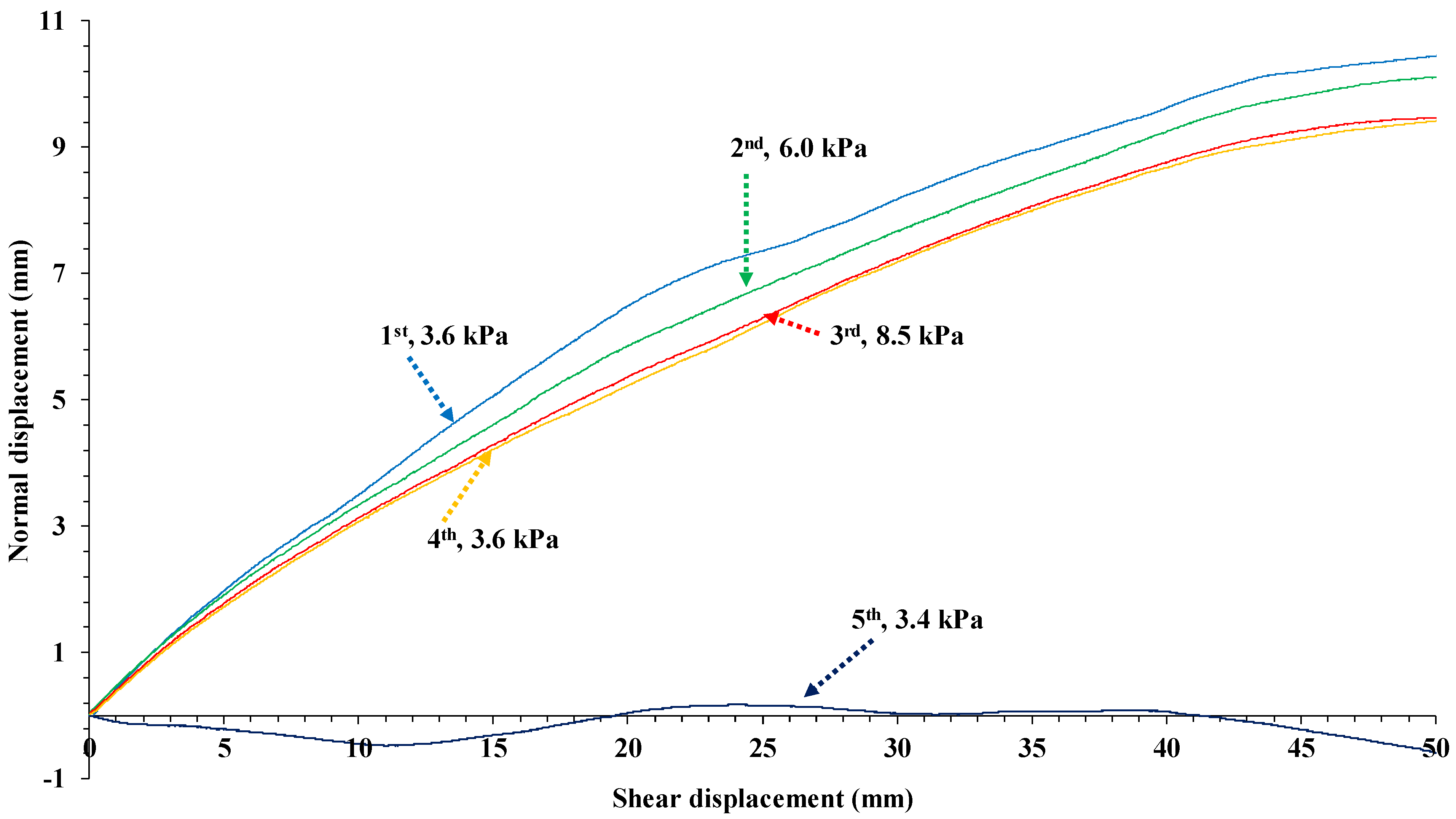
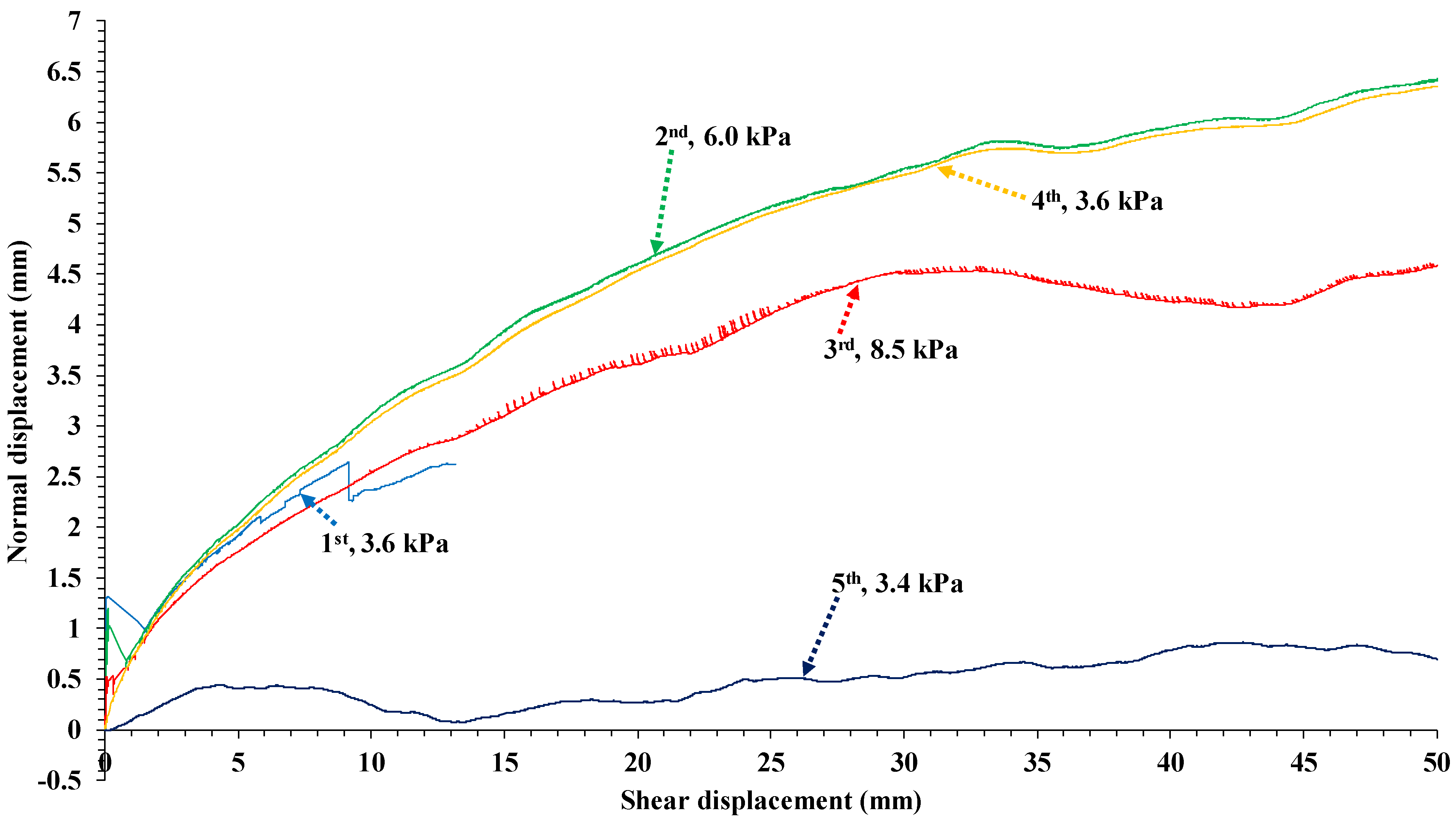
| Phase | Description | Normal Stress (kPa) |
|---|---|---|
| Pre-test | Photogrammetry | |
| First stage: | Pushing without extra normal stress | 3.6 |
| Damage mapping 1 | Visual assessment of damage locations and resetting | |
| Second stage: | Pushing with extra normal weight | 6.0 |
| Damage mapping 2 | Visual assessment of damage locations and resetting | |
| Third stage: | Pushing with extra normal weight | 8.5 |
| Damage mapping 3 | Visual assessment of damage locations and resetting | |
| Fourth stage: | Pushing without extra normal stress | 3.6 |
| Damage mapping 4 | Photogrammetry | |
| Fifth stage: Unmatched residual | Pushing without extra normal stress, top sample rotated through 180° | 3.4 |
| Phase of Shearing Test | Weight (kg) | Normal Stress (kPa) | ||||||
|---|---|---|---|---|---|---|---|---|
| Large Sample Test | Medium Sample Test | |||||||
| Slab | Frame | Additional | Total | Slab | Additional | Total | ||
| First stage | 697.60 | 34.5 | 0 | 732.10 | 17.11 | 28.65 | 45.76 | 3.6 |
| Second stage | 697.60 | 34.5 | 500.23 | 1232.33 | 17.11 | 59.91 | 77.02 | 6.0 |
| Third stage | 697.60 | 34.5 | 1000.20 | 1732.30 | 17.11 | 91.16 | 108.27 | 8.5 |
| Fourth stage | 697.60 | 34.5 | 0 | 732.10 | 17.11 | 28.65 | 45.76 | 3.6 |
| Fifth stage | 697.60 | 0 | 0 | 697.60 | 17.11 | 26.49 | 43.60 | 3.4 |
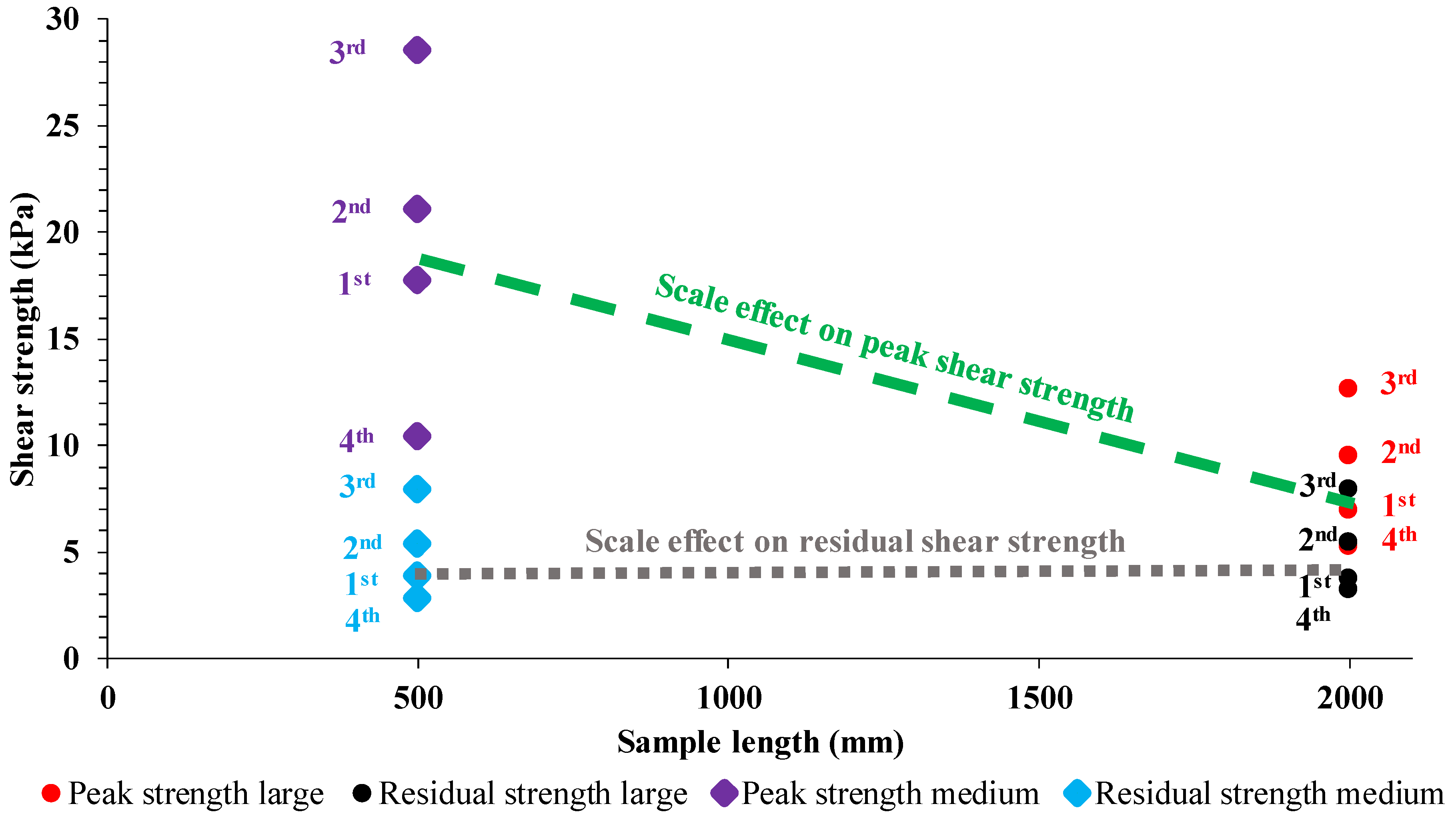
| PHASE | Normal Stress | Large Size Sample 2000 mm × 1000 mm | Medium Size Sample 500 mm × 250 mm | ||||
|---|---|---|---|---|---|---|---|
| Peak Shear Strength | Residual Shear Strength | Shear Displacement at Peak | Peak Shear Strength | Residual Shear Strength | Shear Displacement at Peak | ||
| (kPa) | (kPa) | (kPa) | (mm) | (kPa) | (kPa) | (mm) | |
| First stage | 3.6 | 6.9 | 3.7 | 0.52 | 17.8 | 3.9 | 0.08 |
| Second stage | 6.0 | 9.5 | 5.4 | 0.73 | 21.1 | 5.4 | 0.11 |
| Third stage | 8.5 | 12.0 | 7.9 | 0.68 | 28.6 | 8.0 | 0.07 |
| Fourth stage | 3.6 | 5.2 | 3.2 | 0.50 | 10.4 | 2.8 | 0.10 |
| Fifth stage | 3.4 | N/A | 2.05 | 60.0 | N/A | 2.5 | 1.18 |
| Sample | Peak Friction Angle (°) | Peak Cohesion (kPa) | Residual Friction Angle (°) | Residual Cohesion (kPa) |
|---|---|---|---|---|
| Large sample (2000 mm × 1000 mm) | 53.34 | 1.27 | 41.9 | 0.217 |
| Medium sample (500 mm × 250 mm) | 71.19 | 3.51 | 42.72 | 0.028 |
| Item (Using Barton–Bandis’s Criterion) | Large | Medium | ||||
|---|---|---|---|---|---|---|
| JRC | Peak Friction Angle (°) | JRC | Peak Friction Angle (°) | |||
| Direct shear test | 6.17 | 62.51 | 9.54 | 78.6 | ||
| Profilometer | L0 | 10.5 | 81 | 9.3 | 77 | |
| Lscaled | 5.6 | 59.8 | 6.9 | 66 | ||
| Photogrammetry | Z2 | L0 | 10.11 | 77.53 | 10.88 | 85 |
| Lscaled | 5.5 | 59.3 | 7.7 | 69.8 | ||
| Z′2 | 6.95 | 66.22 | 8.91 | 75.58 | ||
Publisher’s Note: MDPI stays neutral with regard to jurisdictional claims in published maps and institutional affiliations. |
© 2021 by the authors. Licensee MDPI, Basel, Switzerland. This article is an open access article distributed under the terms and conditions of the Creative Commons Attribution (CC BY) license (https://creativecommons.org/licenses/by/4.0/).
Share and Cite
Uotinen, L.; Torkan, M.; Baghbanan, A.; Hernández, E.C.; Rinne, M. Photogrammetric Prediction of Rock Fracture Properties and Validation with Metric Shear Tests. Geosciences 2021, 11, 293. https://0-doi-org.brum.beds.ac.uk/10.3390/geosciences11070293
Uotinen L, Torkan M, Baghbanan A, Hernández EC, Rinne M. Photogrammetric Prediction of Rock Fracture Properties and Validation with Metric Shear Tests. Geosciences. 2021; 11(7):293. https://0-doi-org.brum.beds.ac.uk/10.3390/geosciences11070293
Chicago/Turabian StyleUotinen, Lauri, Masoud Torkan, Alireza Baghbanan, Enrique Caballero Hernández, and Mikael Rinne. 2021. "Photogrammetric Prediction of Rock Fracture Properties and Validation with Metric Shear Tests" Geosciences 11, no. 7: 293. https://0-doi-org.brum.beds.ac.uk/10.3390/geosciences11070293