
Tidal Flood Risk on Salt Farming: Evaluation of Post Events in the Northern Part of Java Using a Parametric Approach


1
Department of Geography, Universitas Muhammadiyah Purwokerto, Banyumas 53182, Indonesia
2
Institute of Geography, Department of Geosciences, University of Cologne, 50923 Cologne, Germany
*
Author to whom correspondence should be addressed.
Geosciences 2021, 11(10), 420; https://0-doi-org.brum.beds.ac.uk/10.3390/geosciences11100420
Submission received: 23 August 2021
/
Revised: 22 September 2021
/
Accepted: 5 October 2021
/
Published: 9 October 2021
(This article belongs to the Collection Early Career Scientists’ (ECS) Contributions to Geosciences)
Abstract
:Tidal flood risk threatens coastal urban areas and their agriculture and aquaculture, including salt farming. There is, therefore, an urgency to map and portray risk to reduce casualties and loss. In the floodplain of Cirebon, West Java, where salt farming dominates the landscape, this type of flooding has frequently occurred and disrupted the local economy. Based on two recorded events in 2016 and 2018 as benchmarks, this paper formulates an innovative approach to analyze tidal flood risk in salt farming areas. Our study considers the fundamental concepts of hazard and vulnerability, then uses selective parameters for evaluation in an Analytical Hierarchical Process (AHP)-based Geographic Information System. The analytical process includes weighting criteria judged by experts and uses the resulting values to define the spatial characteristics of each salt parcel. Our high-resolution simulations show that the two flood events in 2016 and 2018 affected almost all salt production areas, particularly in the eastern, middle, and western parts of the Cirebon floodplain, although to very different degrees. The study also uses a physical-based approach to validate these results. The damage estimates show a strong positive correlation for economic loss (r = 0.81, r = 0.84). Finally, the study suggests that our multi-methods approach to assessing tidal flood risk should be considered in disaster mitigation planning and integrated coastal zone management in salt farming areas.
1. Introduction
Nowadays, millions of inhabitants have been threatened by floods in coastal regions, with the most destructing impacts in rural coastal communities in developing countries [1]. People from lower income brackets tend to settle in floodplains in remote rural areas due to lower land prices and possible cultivation activities [2]. The physical and social settings have turned many of these areas into high-risk regions through geohazards such as tsunamis, storm surges, and flooding. These circumstances are worsening, especially in the Global South, due to limited mitigation capacity [3,4]. At the same time, most of the population in these low land areas is being supported by fisheries [5,6] and agriculture products [7], including salt [8,9].
On the north coast of Java, Indonesia, salt farming has been practiced for hundreds of years. Along the shore, traditional salt farmers have produced the salt brine with inputs mainly from the Java Sea, which has a relatively shallow depth and mostly calm waves. Seawater bitterns are encountered in the sea-salt production and desalination process in which large portions of bittern and brine are processed as by-products and waste products [10]. Besides being used as raw material and for food, the local salt product is also used in the chemical industry. Salt farming in this region is of the local culture. However, the area is also vulnerable to coastal hazards [11,12]. Flooding occurs due to intense rainfall and sea-level dynamics. Extreme sea levels resulting from combined events of high tides and storm surges are considered a significant threat for coastal communities and their infrastructure [13,14].
Tidal flooding has threatened traditional salt farming in Cirebon, West Java, again and again, especially during the production period from April to October. Local and national media have described at least two recent tidal flooding events, in 2016 and 2018 [15,16,17]. Our previous paper modeled those events through a physical-based approach using a numerical model [18]. In the last few years, risk assessment for this type of flood in the north part of Java has been probed in several studies focusing on urban areas using various methods [19,20,21]. One example of a coupled method was practiced in the Eilenburg municipality, Germany. A risk analysis comparison was performed for different scenarios of hydraulic model and flood loss model combinations [22]. The method also involves the Flood Loss Estimation Model for the private sector (FLEMOps) approach and a benchmark from a previous monetary loss estimation by the Saxonian Relief Bank (SAB). In another case study by Ward et al. [23], the damage-scanner model was used to estimate the flood risk through the expected annual damage (EAD) algorithm. That study also addressed the general estimation of different categories based on land use types, including residential, agricultural, commercial, industrial, and recreational. With different flood scenarios in that model, the paper also stated that floods with relatively low economic damage per event should also be considered in the flood risk assessment due to frequency [23,24]. Several of those studies also optimized the use of geospatial technology such as remote sensing and geographic information systems (RS-GIS).
Currently, the established flood risk models focus on urban structures, while agriculture have been hardly discussed [25], with a few studies trying to address the economic impact on agricultural land using different approaches [26,27,28]. However, there are still limited studies concerning the flood risk for agricultural areas including the coastal parts of Central [29] and West Java [30]. Therefore, this article mainly endorses methodological innovation to evaluate tidal flood risk on salt farming land by applying geospatial data and geographic information system technology.
2. Conceptual Considerations
2.1. Concept and Definition of Hazard, Vulnerability, and Risk
The concepts of hazard, vulnerability, and risk are widely discussed in numerous studies on natural hazards and disaster risk management. The following sub-sections describe some relevant theoretical considerations and empirical results from former studies.
2.1.1. Hazard (H)
A natural hazard can be described as the possibility of events of potentially damaging natural phenomena in a particular period and a certain area [31]. The hazard also can be simply defined as a threatening natural event, including its magnitude and probability of occurrence [32,33]. Hazards can contain latent conditions that may characterize future threats and can have multiple causes, including natural (geological, hydrometeorological, or biological) and anthropogenic processes (environmental degradation or technological hazards) [34]. Each hazard is characterized by its specific geography, intensity, regularity, and probability [35].
Hazard assessment has been conducted in many different areas including coastal regions, with a pronounced focus on hydrometeorology hazards such as cyclones, storm surges, and flooding. Flood hazard measurement aims to identify the flood pattern utilizing relevant parameters such as inundation depth [36,37,38], flood duration [38,39,40], and even timing of flooding [41,42,43]. This information can be extracted through hydraulic models with different scenarios [44] or based on past recorded events [45,46].
2.1.2. Vulnerability (V)
Researchers define vulnerability in diverse spatial contexts, for different purposes, and with different rationales [47]. It is widely accepted, however, that vulnerability is a condition influenced by physical, social, economic, and environmental factors that raise the susceptibility of people to a hazard impact [48]. In an engineering conceptualization, vulnerability defines the scale of the region, population, physical structures, or properties exposed to the hazard [49]. Thouret et al. [50] extended the description of vulnerability as a degree of damage to a certain object at flood risk by including a specified amount, expressed on a scale from 0 to 1 (no damage to full damage).
Vulnerability should be able to portray the specific problem in the context of a locality [51]. At some points, it is also understood that vulnerability is a relative concept that relies on the society’s interpretation of a risk and how communities construct their normality on a daily basis [52]. Previous studies obtained vulnerability measures through selecting relevant parameters, i.e., they focused on the watersheds involving hydrologic and physical components such as elevation, slope, geomorphological conditions, soil, and land use [53,54]. In coastal areas, the specific characteristics of additional parameters, such as coastal slope, distance to the next channel, and distance to the sea, are used [55,56,57,58].
2.1.3. Risk (R)
The concept of risk is broadly discussed in various contexts and with various purposes. Risk is commonly associated with hazard (H) and vulnerability (V), especially in the field of flood risk management. In many cases, the simple equation (Equation (1)) is illustrated as follows [34,59,60]:
R = H * V
UNISDR [59] defines risk as a combination of the probability of a hazardous event and its consequences, which result from the interaction between natural or man-made hazards, vulnerability, exposure, and capacity. In this context, the concept of flood risk is closely interrelated to the probability that a high flow event of a given extent happens, which results in specific environmental, financial, and social deficiencies [47]. In addition, risk is also dynamic due to the different ability of the society and environment to manage and adapt to the changes [42].
The selection of instruments and approaches for risk analyses mainly relies on the objective and existing information about the hazard and the vulnerability [60]. As risk is the combination of hazard and vulnerability, the expected damage can be evaluated by a value combination of the elements-at-risk and the estimated damage function [61]. The current practice of risk assessment including flood hazards and cost-benefit analyses focuses on damages that can be easily assessed in monetary terms [62]. Currently, the coupled flood loss estimation and risk assessments have been practiced in residential areas [63].
2.2. Flood Risk Assessment Using a Physical-Based and Multicriteria Approach
Different methods in addressing flood risk have been advanced [64,65]. According to Balica et al. [47], there are at least two distinct techniques in flood risk assessment. First, the deterministic approach, which applies physical-based numerical modelling to calculate flood hazard probability, coupled with a damage estimation model that describes the economic loss. This information can be used for flood risk assessments for particular regions. Studies that integrate a physical-based flood simulation and a damage estimation model have been conducted in different regions, usually with a focus on agriculture [26,36,38,66]. The second technique is the parametric approach, which uses available datasets to describe the relevant hazard and vulnerability features in a study area [47]. This approach involves experts in hazard and vulnerability assessment generating a straightforward risk map based on available data [67]. This method has been applied mainly in data-scarce regions or developing countries.
Recently, the combination of different geospatial data series with a multicriteria approach (MCA) has contributed to flood vulnerability and risk assessment [66]. MCA is a suitable method for all relevant types of impacts, without any measurement on a single monetary rank [68]. The integration of MCA and Geographic Information Systems (GIS) enhances the utilization of the three components of risk (hazard, vulnerability, and exposure), including social, economic, and/or environmental vulnerabilities [69]. GIS are eminently suited to processing the geospatial data required for flood risk assessment. This technology is also acknowledged for its great flexibility in MCAs, including the very reliable analytical hierarchical process (AHP) [31,70,71,72]. This semi-quantitative approach has its strength in supporting priority selection and decision-making [39]. The method has been widely recognized in the academic literature and has been recently applied in studies on flood risk assessment [73,74]. In the present study, AHP was performed and utilized to evaluate the tidal flood risk in salt farming areas through thematic data layers processed on a GIS platform.
3. Description of the Case Study Area
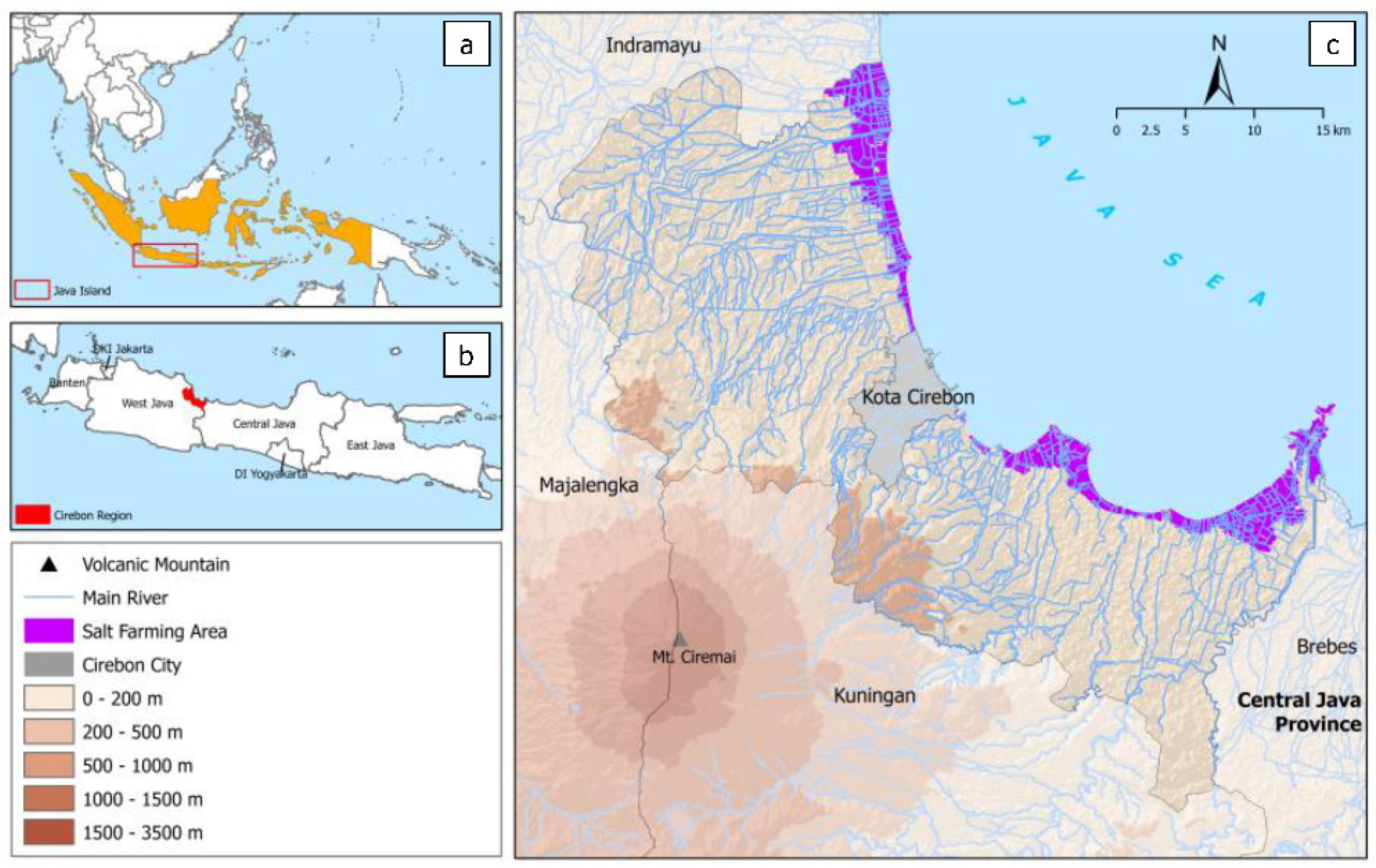
The coastal area of Cirebon, West Java, Indonesia has been acknowledged as one of the major centers for traditional salt production in Indonesia. The region covers around 990 km2 between 6°30′ and 7°00′ S and 108°40′ to 108°48′ E. The Cirebon borders of the province of Central Java are on the east, the Java Sea is to the north, and Indramayu is to the west. Cirebon has 40 districts, with eight located along the coastline. According to the Development Planning Board [75], the coastal water area covers 399.6 km2. The region is geomorphologically diverse, with mountainous areas and also coastal plains (Figure 1). As mentioned by Hadian et al. [76], the region consists of four geological units: alluvium deposits, coastal deposits, results of the young Ciremai Volcano, and the Gintung Formation. The coastal area is structured by mud sediments, silt, and grey clay containing shells that are deposited several meters thick. Mount Ciremai (3078 m) is an active stratovolcano and one of the highest active volcanoes in Indonesia. Slope conditions in Cirebon predominantly consist of flat zones (less than 5°), but there are also moderate (5–30°) and steep areas (more than 30°) [77].
Salt harvesting predominantly takes place in low-lying areas dominated by alluvial deposits together with mangrove ecosystems along the Cirebon shoreline. The local farmers benefit from tidal cycles that supply the salt ponds with sea water. Solar energy is used to evaporate the sea water into salt brine, especially during the dry season. In this region, the dry season usually lasts from March to September, while the rainy season begins in October and ends in February, with 1300–1500 mm/year of rainfall and a mean temperature of 24.2 °C [78]. Most farmers start to store seawater at the beginning of the dry season. In that period, the mean temperature is 32.8 °C with a maximum average temperature of 38.6 °C in October [78]. As the dry period begins, the brines are formed in the crystallization pond. Local farmers start to collect brine and produce 0.5–1.0 tons per hectare each day [18,79]. During the production season in 2019, Cirebon produced at least 135.9 thousand tons of salt [78].
4. Research Materials and Methodology
4.1. Model Framework
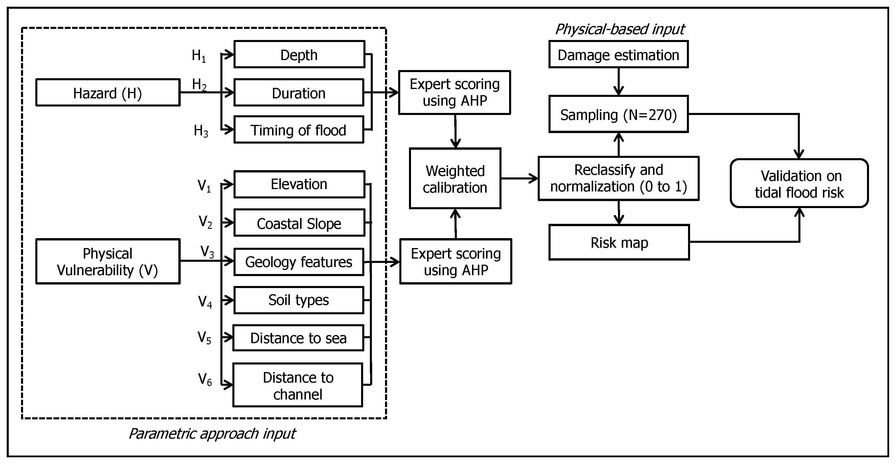
This study evaluates the tidal flood risk using a parametric approach: the analytical hierarchical process (AHP). In addition, we compare the AHP results with the results of a physical-based model. For this purpose, several indicators from geospatial data and relevant research were carefully chosen to identify risk components. A total of 9 indicators were selected and arranged into two clusters of risk components. The first cluster consisted of hazard (H) indicators (n = 3; explained in Section 4.2), and the second compiled vulnerability (V) indicators (n = 6; described in Section 4.3). The selected indicators were used in the AHP analysis to acquire the weighted score (illustrated in Section 4.4). All selected indicators in each thematic layer were processed using ArcGIS 10.6. All maps were set on raster format with a 25-m cell size, Universal Transverse Mercator (Zone 48S) projection, and reclassified to optimize the calculation. Ultimately, the risk map gained from the weighted score calculation was validated using a physical-based approach from a former study (elaborated in Section 4.6). These data allowed an individual analysis of each pond in the risk analysis with the chosen parameters. Additionally, the cell size was customized into 25-m for the purpose of synchronization with the former study. Figure 2 depicts the study’s structure.
4.2. Tidal Flood Hazard Components
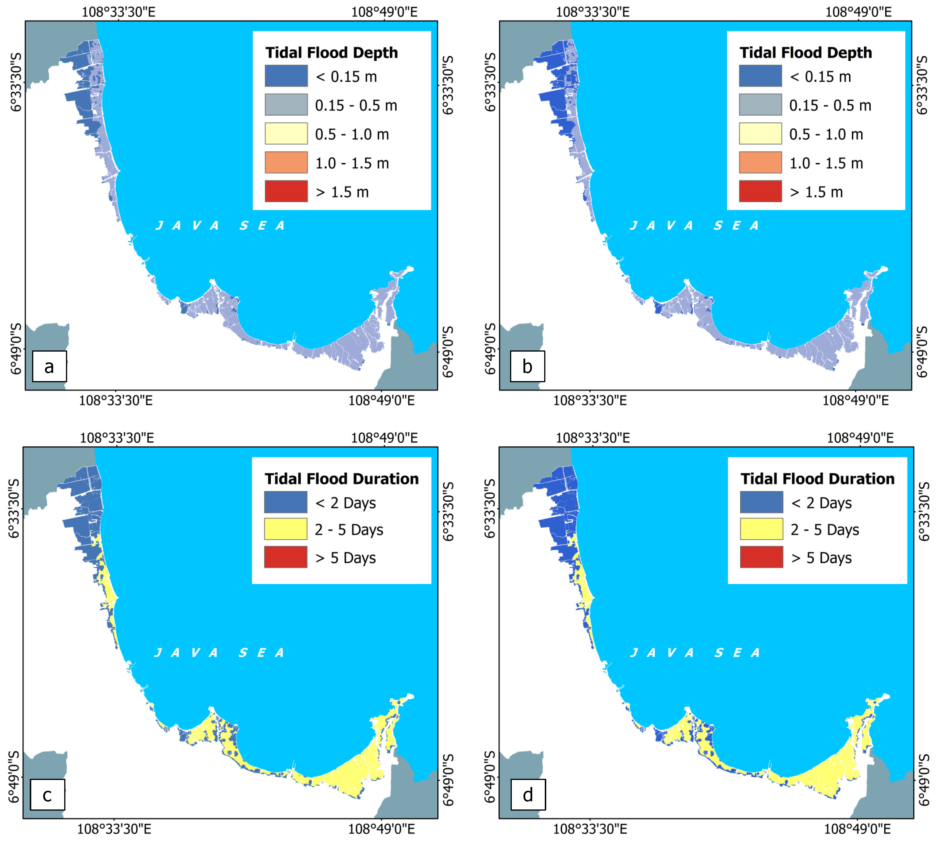
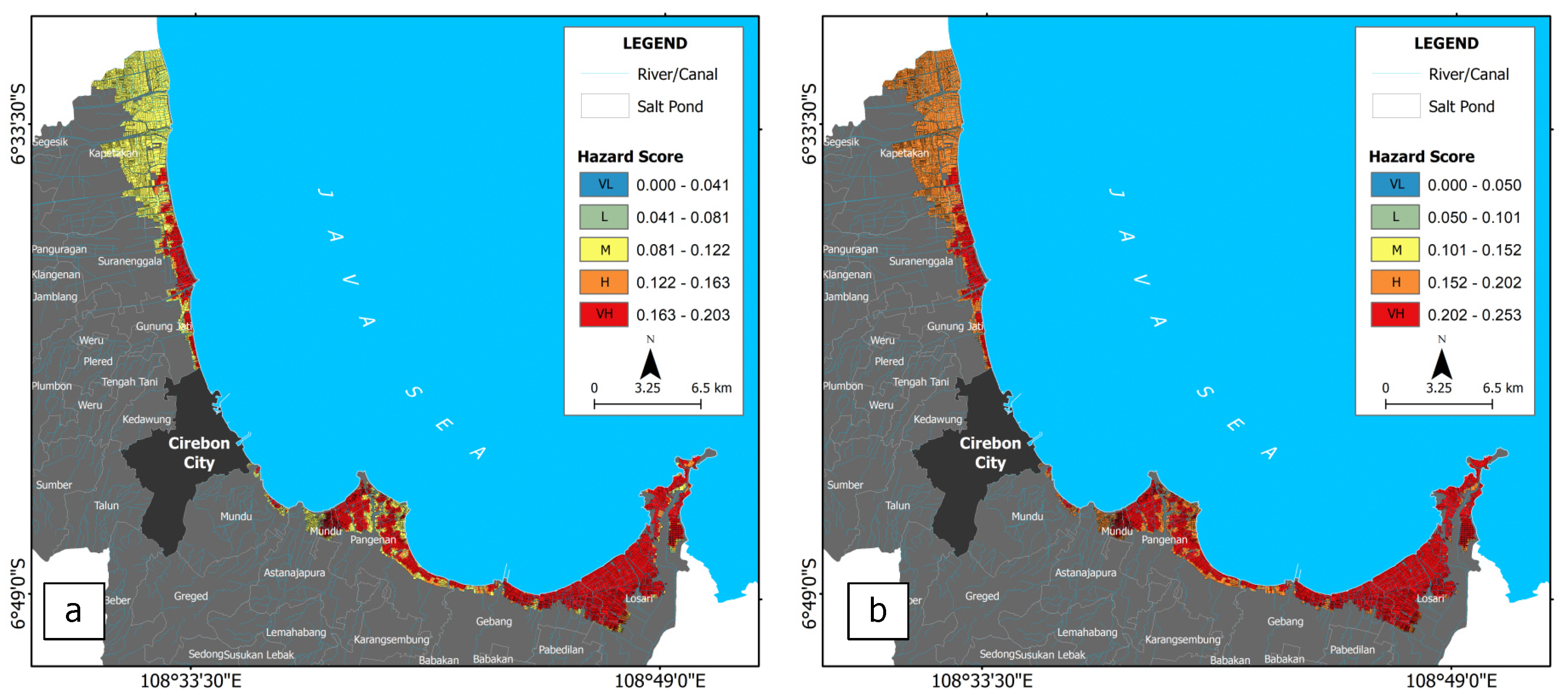
Tidal induced hazards have disrupted most of the coastal communities, including salt farmers, in the Cirebon region. This current study uses two recorded events in 2016 and 2018, with 0.38 m and 0.40 m depth, respectively [18]. Those depths were extracted by Nirwansyah and Braun [18] through a hydrodynamic model in DHI MIKE. However, the events occurred at different stages of salt production. The hazard (H) indicators or criteria (shown in Figure 3) include the following primary factors: (i) The depth (H1) was mainly extracted from the magnitude of the tide. The flood hazard increased proportionally to the depth of inundation [80]. The previously mentioned simulation was reclassified into 5 classes (<15 cm; 15–50 cm; 50–100 cm; 100–150 cm; >150 cm) to be judged by selected experts. (ii) The duration (H2) of the tidal floods was 2.23 days for 2016 and 2.32 days for 2018, for the events analyzed in the study by Nirwansyah and Braun, respectively [81]. In that model, the duration was extracted from individual raster data from hourly hydrodynamic simulation that exported in ArcGIS. We classified the duration of inundation into 3 categories (<2 days; 2–5 days; and >5 days). The duration of flooding is associated with the possible damage level [82,83]. In salt farming, the duration of flooding increases the risk that the formed salt brine melts [81]. (iii) The time of flood (H3) is significant for flood damage in farming activities [41]. As mentioned in the previous section, the time dimension has a strong impact depending on the particular event and the response from the environment or community [23]. For this study, the selected indicators were divided into 3 groups (pre-production, harvesting period, and post-production). The event in 2016 occurred during the harvesting period, whereas the 2018 flood happened in the pre-production period.
4.3. Vulnerability Components
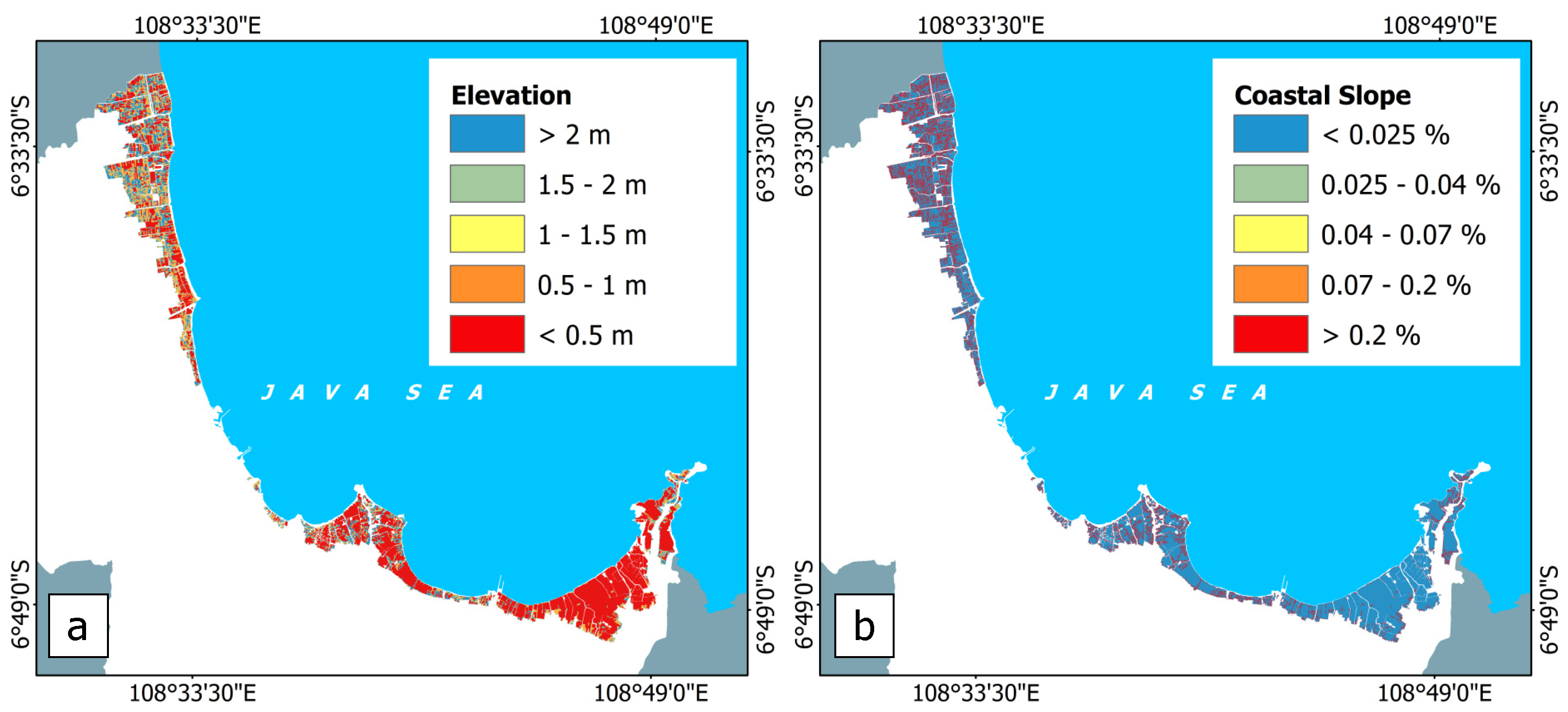
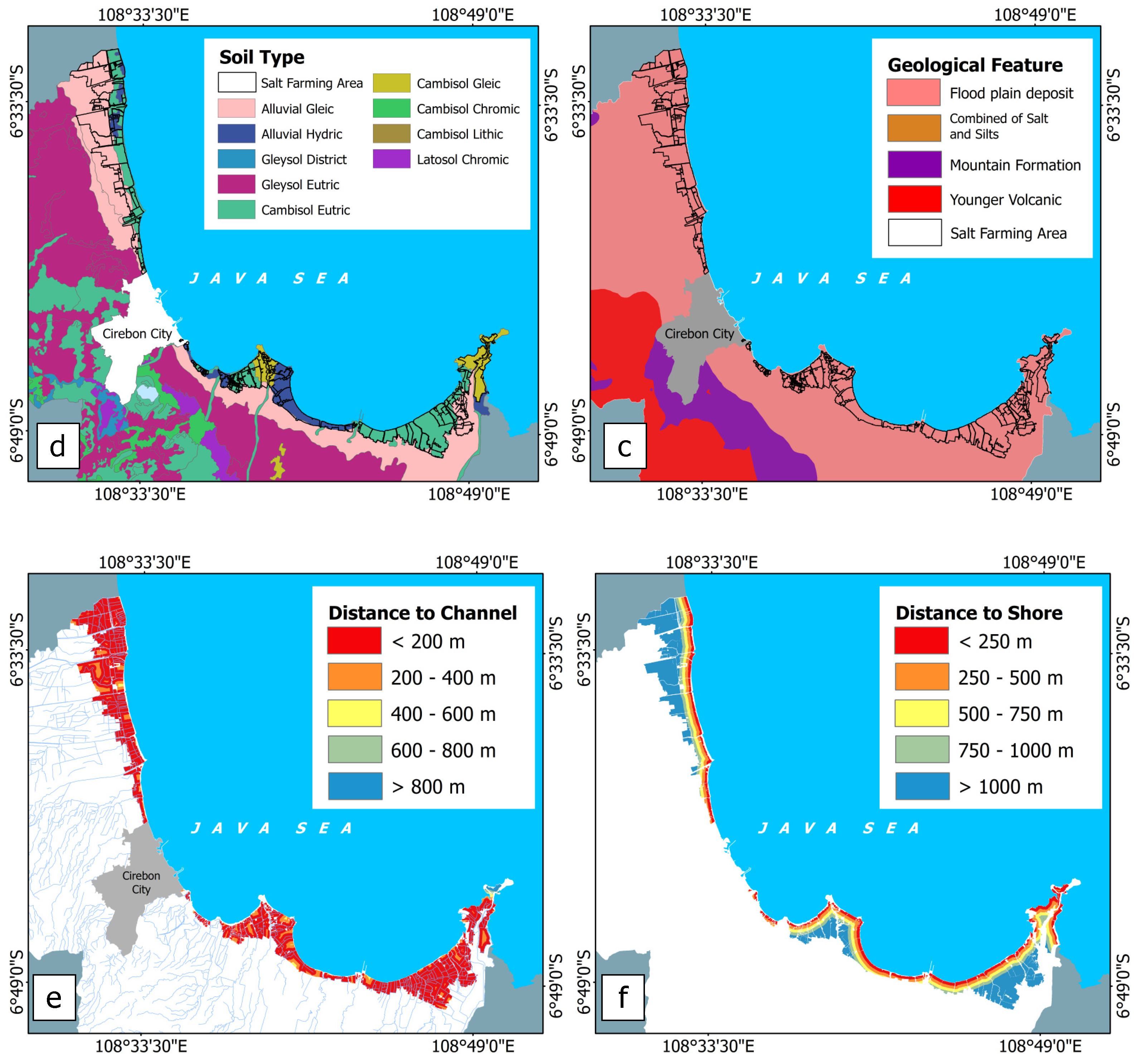
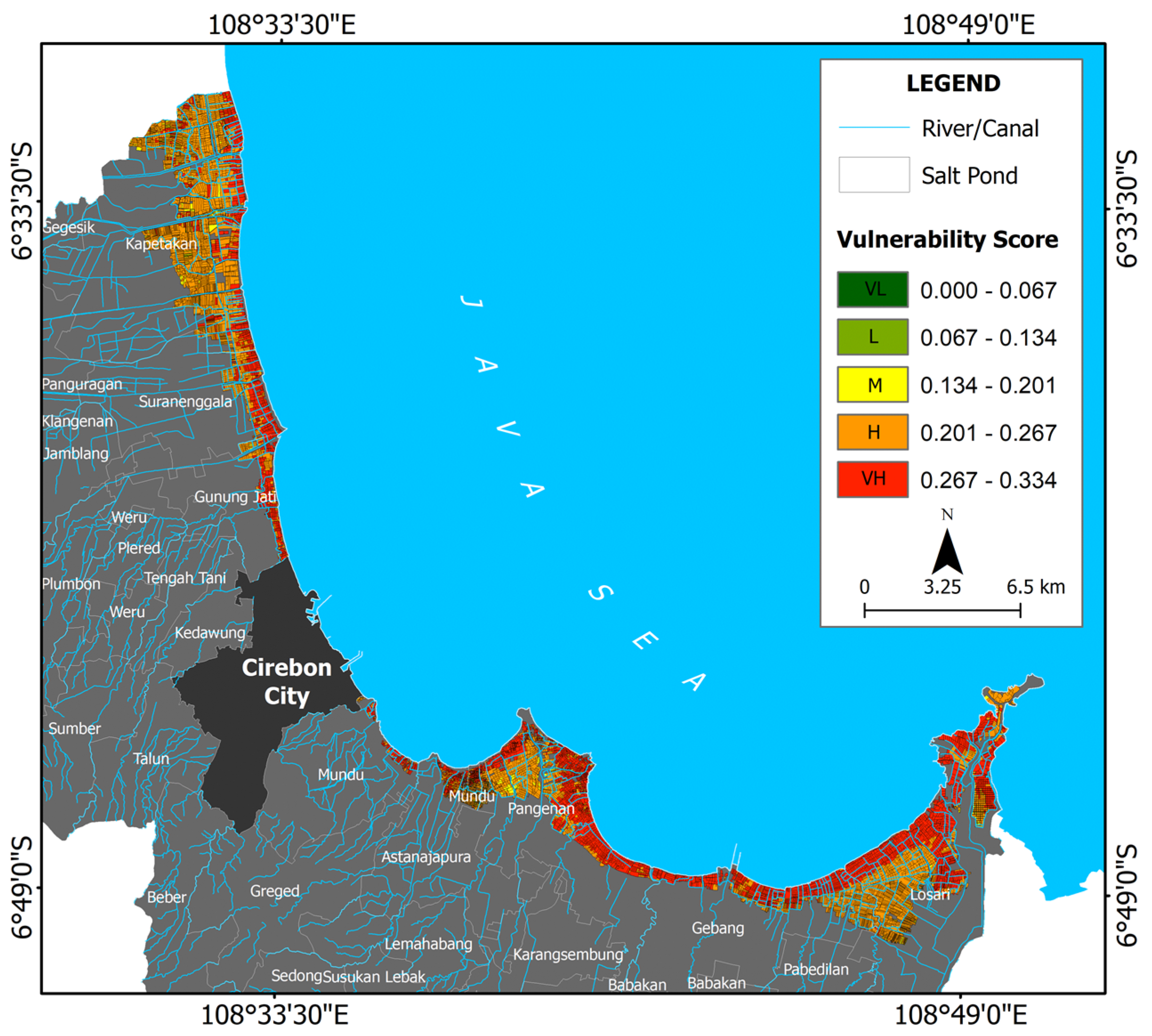
To investigate the vulnerability in coastal zones, a range of parameters and indexes, including physical vulnerability, can be applied [57,84]. Several parameters were used to address the vulnerability components (V). These are shown in the thematic maps (Figure 4). Firstly, (V1) elevation data were extracted from topographical data of DEMNAS (0.27 arc-second) resolution from the Geospatial Information Agency (here referred to as BIG: Badan Informasi Geospasial). The elevation has been categorized into 5 groups (0.5 m; 0.5–1 m; 1–1.5 m; 1.5–2 m, and >2 m). This information generally depicts the coastal altitude conditions [39,69]. This component plays a significant role in identifying areas at risk of flooding during an event [85]. Salt farming is mostly located in the coastal plain within 1–2 m elevation. The variable coastal slope (V2) indicates the degree of elevation variability in bordering grids [86]. The possibility of flooding rises as the slope declines, making it a relevant indicator for vulnerability [87]. Salt ponds require a relatively slight slope to facilitate the sea water flow and to reduce construction expenses [88]. In line with Silva et al. [54], the slope in the case study area was classified into categories of <0.025%, 0.025–0.04%, 0.04–0.07%, 0.07–0.2%, and >0.2%. Another considered indicator, geological features (V3), significantly influences the drainage pattern formation associated with the floodplain formation [89]. In this study, specific classes were included: flood plain deposits, sand with silts and clays, mountain formations, and younger volcanic formations. This classification was taken from the Directorate of Geology and Environmental Planning (DGTL) vector data. Soil type (V4) is a relevant factor affecting infiltration and runoff during floods [71]. In traditional salt farming, salt production has major implications for productivity, water quality, and pond construction [90]. The DGTL soil map, scale 1:100,000, reveals that the soil of the Cirebon region is divided into four major types, Alluvial, Gleysol, Cambisol, and Latosol, although the salt pond area is dominated by Alluvial soil. This dominant soil type is the result of sedimentation from streams and rivers or of marine sediments along ocean shorelines [91]. To identify the soil characteristics, Subardja et al. [92] and Sulaeman et al. [93] were used as sources for this study. Finally, both distance to channel (V5) and distance to shore (V6) influence the breaching of water during floods and overtopping water from the channel. This study classified distance to channel into <200 m, 200–400 m, 400–600 m, 600–1000 m, and >1000 m [94], and distance to shore into <250 m, 250–500 m, 500–750 m, 750–1000 m, and >1000 m. All mentioned classification references were defined in the level of vulnerability to tidal flood events.
4.4. AHP and Variable Weighting Procedure
In various flood risk studies, the analytical hierarchical process (AHP), introduced by Saaty [95], has been effectively used to conduct flood risk measurements [70,72,96]. This method selects criteria by ranking the parameters and creating a combination of qualitative and quantitative factors [39,56,69]. Generally, this approach is a structured technique to deal with complex decisions and to help decision-makers find the most suitable options [97]. In this process, the decision-makers use factual data related to the included elements and can use their professional judgments to identify the level of importance by using a basic scale of absolute numbers (listed in Table 1).
The AHP was employed to obtain the weight scores of selected criteria and sub-criteria based on an evaluation by the interviewed stakeholders and experts associated with the policy-making process [39]. Following Cabrera and Lee [71], four experts from local authorities, including the Ocean and Fisheries Department (DKP) of Cirebon, the Indonesian National Geospatial Agency (BIG), the Spatial Planning Official (BAPPEDA) of the West Java province, and an academic from the geomatic department, Brawijaya University, were involved due to their experience and their duties regarding salt farming. These experts carefully judged all parameters and the H, V, and R indicators. Due to the COVID-19 pandemic, data collection was conducted via online correspondence using Zoom from January to March 2021. The collected data were inserted into a template (https://bpmsg.com/, accessed on 10 January 2021) containing the AHP justification variables. This Excel workbook consists of 20 input worksheets for pair-wise comparison [100].
In the present research, AHP was employed to allocate weights for the H, V, and R factors. The following steps were included in the AHP: A pairwise comparison was performed for all H, V, and R indicators and a matrix was established through scores based on relative importance. A pairwise comparison matrix was utilized to compare and rank the selected H and V domains based on the experts’ judgments. The assessment was based on the relationship between the indicators and the risk components. The indicators were reclassified and ranked. Here, different ranks were applied from 1 to 3, 1 to 4, and 1 to 5. Finally, the normalized rank was counted by dividing the column value by the sum of the ranking’s score. After doing so, the total score for each indicator was 1. Table 2 represents the rankings and the normalized scores of all selected indicators used in the present work.
In the AHP model, the Eigenvalue of the matrix expresses the priority value of variables [31,56]. The estimations were completed by dividing each column by the value of their sum [69]. Ultimately, the mean values of each row were carefully estimated and used as weights in the objective hierarchy in the H and V domains. In addition, to establish the consistency of the comparison matrix, a standardized Consistency Ratio (CR) test was generated. The ratio confirms the justification or preference to be consistent if the CR < 0.10, and reliable results can be supposed in the model [101]. However, a greater CR value does not necessarily mean a greater accuracy [39]. The consistency ratio test is formulated in Equation (2)
where CI is described as the consistency index and RI refers to a random index whose value is stated by the number of criteria (n) [72]. The consistency index is expressed as follows in Equation (3).
CR = CI/RI
CI = (λmax–N)/(N–1)
Here, λmax represents the maximum Eigenvalue of the comparison matrix while n describes the number of criteria for each variable of H (n = 3), V (n = 6), and R (n = 2). In the present study, the CR and CI for H were calculated as 0.012 and 0.03 while the RI was 0.58. For the V variable, the CR was estimated as 0.019, the CI was measured as 0.07, and the RI was 1.24. The value of the RI standardized in the AHP was taken from Table 3.
4.5. Estimating H, V and R Tidal Flood Indices
A composite risk map (R) in the raster data format was expected to be the result of this model in 25-m cell size. The weight input from the previous process in the AHP was used to construct the mathematical formulation with H and V criteria (see Equations (4) and (5)). The weight score from previous expert inputs and the calculations were combined using weighted overlay in ESRI ArcGIS 10.6, which generated hazard maps (H) for the 2016 and 2018 cases, in addition to a vulnerability map (V), by means of map algebra tools in the software. The risk assessment result was incorporated into a GIS platform to provide a flood risk map [80]. The following expressions describe the risk as the ultimate result of the MCA approach for H and V with incorporated expert judgment.
H = 0.109 × H1 + 0.567 × H2 + 0.324 × H3
V = 0.161 × V1 + 0.137 × V2 + 0.086 × V3 + 0.11×V4 + 0.265 × V5 + 0.241 × V6
In line with Equation (6), the R is measured by combining both the H and V inputs. Here, both weighted components were calculated using a similar procedure in ArcGIS 10.6. In the final map, the scores of risk are normalized into a 0 to 1 range [103]. The results of the weighted overlay analysis were classified using equal intervals, i.e., five levels: very low (0–0.20), low (0.20–0.40), moderate (0.40–0.60), high (0.60–0.80), and very high (0.80–1.00).
Composite of R index = 0.39 × H * 0.61 × V
For the calculation, a salt parcel shapefile in 1:15,000 scale acquired from National Geospatial Agency was used to extract raster values using a zonal statistic operation in ArcGIS.
4.6. Relationship between the Multi-Criteria and Physical-Based Approach
Previous comparison analyses have been presented in established damage models, e.g., those included in [104,105]. However, there is still no direct evaluation of the relation between economic loss from a physical-based approach and risk value from a MCA, especially with regard to salt farming land. Although this combined approach was implemented previously in Afifi et al. [63], no specific correlations were performed. In the study, the simple correlation was obtained in order to evaluate the relation between risk level and monetary damage for both tidal flood events. Since there were no approved reports from the responsible authorities for both recorded tidal flood events, approximately 270 salt parcels were taken as samples according to the proportional number for each risk class, while the damage calculation was taken from the previous numerical model by Nirwansyah and Braun [81]. These parcels contain information on the monetary damage for both selected periods. For this purpose, we used the ‘create random points tool’ in ArcGIS and extracted values from parcel data in vector format using the ‘identity’ feature. The monetary loss was evaluated using the depth-duration damage function taken from Nirwansyah and Braun [81] and was then compared to the scores of both risks. Following Molinari et al. [106], a simple Pearson correlation coefficient (r) was applied to identify both approaches’ relation to each other in a statistical context.
5. Results and Discussion
5.1. Tidal Hazard on Salt Ponds
In this study, the indicators from the selected variables (H1-H3) were processed following the conditions of tidal flooding records in 2016 and 2018. Two hazard maps can be drawn from the model that portrays the tidal occurrence during those two events. The interviewed experts believe that duration (H2) has the most significant impact on the tidal flood hazard (0.567 weight score). Depth (H1) and the timing of flooding (H3) have the least effects on salt farming, according to our experts. The indicators have, respectively, 0.109 and 0.324 weight scores in Equation (4). The hazard map features five classification areas from very low to very high, as shown in Figure 5a,b. For the 2016 hazard, the very low (VL) class extends over 43.63% of all salt ponds, while in 2018, about 42.43% fall into this class. Moreover, about 3.33% of the production area has been grouped in the low (L) class for 2016, and 3.20% for the 2018 event. These areas experience relatively low depth and short inundation during the floods in both tide events. Some districts such as Kapetakan and Suranenggala (west part) have been allocated to this class. Small areas in the districts of Mundu and Pangenan (middle part) have also been allocated to this class. The moderate class (M) covers 3.12% (2016) and 3.74% (2018). The class for very high (VH) hazards comprises 45.59% (2016) and 47.24% (2018) of the total salt farming land in Cirebon. These two classes essentially displayed higher depths and relatively longer durations in 2016 and 2018. Both flood events have mostly affected the eastern part of the region, including Losari, Gebang, and the middle part, including Mundu and Astanajapura.
5.2. Tidal Flood Vulnerability of Salt Ponds
The five combined vulnerability indicators (V1–V5) are shown combined in a single vulnerability map (Figure 6). The experts agreed that each indicator shows a quantifiably different response to tidal flood hazards. Equation (5) clearly shows that the distance to the next channel has been considered as the most influential factor for tidal-induced flooding (26.5%). On the other hand, experts suggest that geological features have the least contribution to the vulnerability level of salt farming due to tidal flood (8.6%). The area with a very low (VL) vulnerability represents only 0.46% of the total salt pond area. This category is essentially dominated by areas with relatively higher elevation, steeper slopes formed by flood plain deposits, mixed types of soils (Alluvial, Gleysol, and Cambisol), and a location far from a channel and the shore. No area is labeled as low (L) vulnerability and only 2.07% are assigned to the moderate (M) class. The H and VH classes represent 57.03% and 40.44% of the salt pond areas, respectively. These classes dominate in almost all salt production areas, including the western, eastern, and middle parts. The analysis shows that all of these areas are characterized by low elevation, flat flood plain deposits, and Cambisol and Alluvial soils. They are also located close to channels and the sea. Not surprisingly, these categories apply to highly productive areas where farmers can easily extract saline water directly from the ocean and transfer it to their ponds.
5.3. Tidal Flood Risk of Salt Ponds
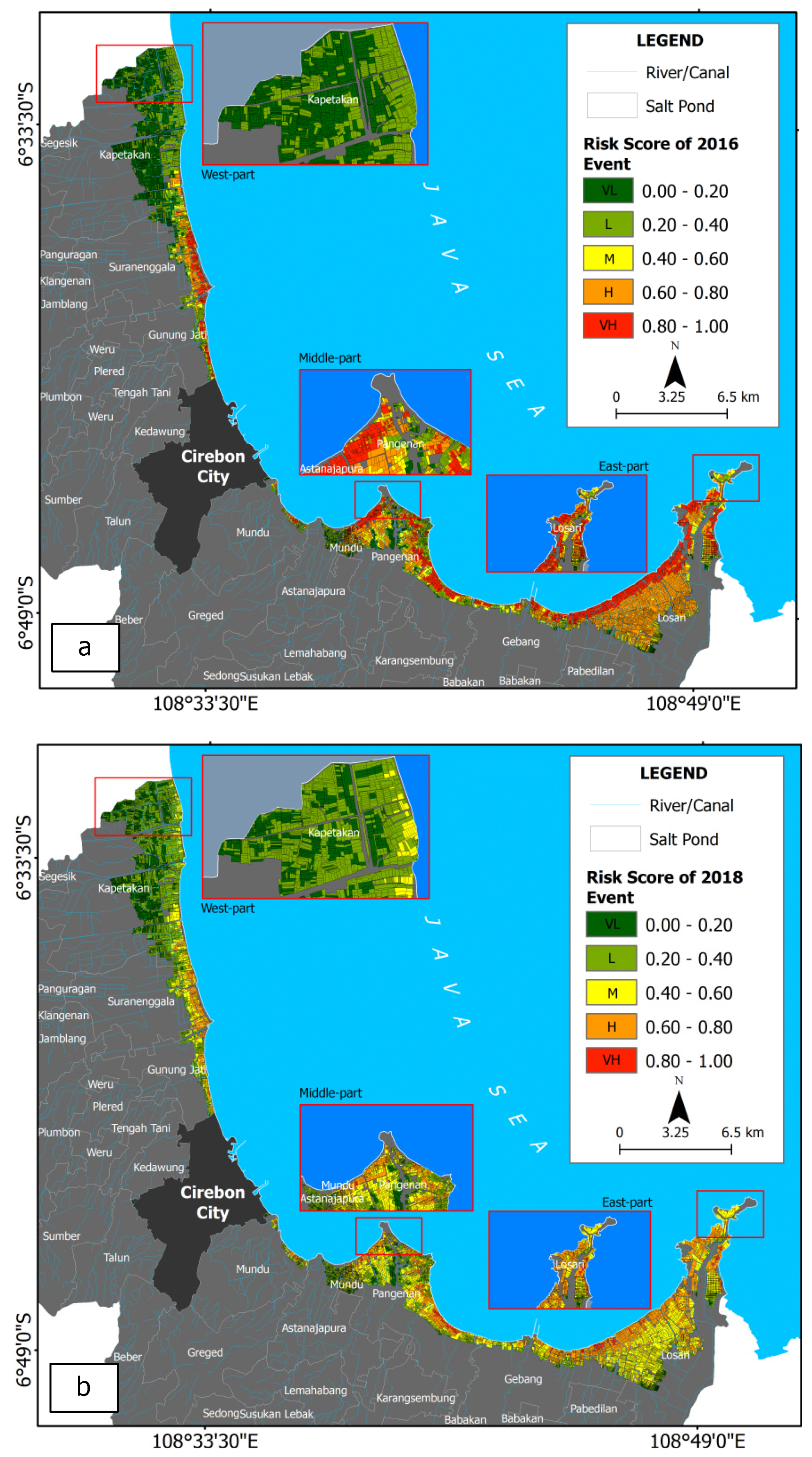
The tidal flood risk (R) map combining the H and V layers outlines five levels of risk, varying from very low to very high (VL to VH). In addition, the V element plays a bigger role than H for the tidal flood risk in salt farming, as described in Equation (6). Here, the interviewed experts have suggested a proportion for both components, where H and V, respectively, contribute 39% and 61% to the resulting risk. The two studied events also present different stages of farming. Our calculations reveal that VL represents 4.06% and 12.72% of the study sites for the 2016 and 2018 floods, while L extends to 15.13% and 33.36% of the total salt farming area, respectively. Areas in these two categories had minimum flood depths and durations. Moreover, these areas are mostly located on higher elevations, have relatively steep slopes, and are far off channels and the shoreline. They are characterized by mixed soil types and were formed by flood plain deposits. They can be found especially in the western part of the region; for instance, in Kapetakan (see top box in Figure 7a,b). The moderate (M) category of risk covers 18.02% (2016) and 30.52% (2018) of the total area of salt farming in Cirebon, while the H class accounts for about 38.54% (2016) and 21.9% (2018). The VH class represents 24.26% of the area for 2016 and only 1.5% for 2018. The H and VH areas had maximum flood depths and durations. This aspect is also physically illustrated by low elevation flat slopes and proximity to the shore and channels. Furthermore, these areas have mixed soil types and geological features dominated by flood plain deposits. Usually, traditional salt farmers tend to choose this type of location due to impervious soil that is suitable for the salt pan surface layer. In Cirebon, these two classes dominate the eastern and middle part, including Losari, Gebang, Pangenan, Mundu, and Astanajapura. Figure 7 shows the levels of risk in the salt farming area of Cirebon based on tidal flood occurrences in the past.
5.4. Validation
Although there are no official reports on the two flood events in 2016 and 2018, previous numerical simulations have to be taken as an alternative to validate the model [81]. According to that study, the total damage value was 170.3 billion rupiahs in the pre-production period, where the salt had not yet been produced, while the total value during the harvesting period was estimated at 1.38 trillion rupiahs [81]. This value includes all costs and lost revenues (C/R) of the production for the whole area. The Pearson value shows strong correlations: in 2016 (harvesting period) the value was 0.81, and in 2018 (pre-production period) the value was 0.84. These strongly positive correlations are associated with monetary loss that was estimated based on the numerical model and the risk score of the current approach. Nevertheless, the impact on monetary aspects has proven to be similar to the one given in the previous model by Nirwansyah and Braun [81].
The maximum loss on each parcel is estimated to be 13.29 million rupiahs (2016 event) and 2.49 million rupiahs (2018 event). Both calculations are close to the physical-based model, where a monetary loss of 13.32 million rupiahs for the 2016 event was calculated and the 2018 event showed a 2.58 million rupiahs loss on the most affected parcel. Table 4 compares the evaluation of the current multicriteria approach with that of the physical-based method.
5.5. Discussion
5.5.1. Implementation of AHP for Tidal Flood Mapping in Salt Farming
This study presents the assessment of risk for salt farming in Cirebon through a combination of hazard and vulnerability parameters. The selected events in 2016 and 2018 showed a relatively low level of risk caused by the hazard magnitude (H), which ranged between 0.203 and 0.253, while the maximum vulnerability (V) score reached a level of 0.334. However, both components highlighted the higher risk areas, especially the ones close to the coast and/or to channels, where the salt ponds were impacted the most (see Figure 8). In extreme cases, the risk can increase drastically due to maximum tides coupled with storm surges, river floods, and sea-level rise [107,108]. Such a scenario will potentially trigger massive disruptions in almost all salt production areas that have minimum structural protection. We expect that our model can be applied to different periods and geographical contexts. Moreover, to assess flood risk in salt farming, several other scenarios of depth and duration are also possible, especially when the absence of historical data records needs to be overcome.
In this study, a combined AHP-GIS approach was implemented to address the tidal flood risk for salt farming. The AHP approach has been efficiently and successfully implemented in other flood risk assessments [31,69,70,71,72]. This approach involves depth and duration as common aspects in flood hazard assessment. We introduced the timing of flooding as an additional indicator as it allows for different responses on each salt production stage. The present study also underlines that vulnerability has a higher impact on flood risk in salt farming compared to the hazard level. This is especially true for factors such as distance to channels or distance to the coast. Other physical conditions such as geological features, soil types, topography, and coastal slopes have less implications for salt farming vulnerability. Although several studies suggest that elevation and slope elements have a substantial impact on coastal vulnerability assessment (CVA) [109,110,111], we argue for considering other parameters in further research, such as the shoreline change range [112,113] and rates of sea-level rise, the latter being a global phenomenon that will increasingly impact agricultural activities in coastal areas throughout the world [114,115].
5.5.2. Combined Parametric and Physical-Based Approaches
The physical-based model, with the advantage of being able to simulate flood occurrences, was used in validating this study. The physical-based approach could compensate for a lack of official damage reports for coastal agricultural land in Cirebon, and is, additionally, a solution to handling the complicated and coupled sets of equations, especially in hydrodynamic processes such as flooding [47]. This approach considers the hydrodynamic condition of the tide that influences the magnitude, the momentum, the tidal character, and the velocity and timing of the stream [116]. However, our model requires various historical data that might be unavailable in many less developed regions. The parametric approach was designed for these situations in order to address hazards and vulnerability through selected, commonly available indicators. Our study also applied a weighting technique, as it proposed the consideration of inter-dependency among variables in the final expression [46,117]. Finally, the study explored the accuracy of both approaches by applying a simple statistical correlation analysis (see Supplementary Material Table S1).
5.5.3. Possible Uncertainties
Many studies appreciate how the AHP can give a better understanding of the topic, especially with a weight given to each indicator [71]. However, there are possibilities for several uncertainties for the current study. First, it was noticed that the elevation data caused uncertainty in the risk model due to errors and extreme smoothing [118]. Although this study used DEMNAS elevation data with a relatively fine resolution, there is possible space for uncertainty in comparison to real salt farming conditions. Second, the subjectivity inherent in the AHP weighting, as it depends on expert opinion in scoring variables [40,71], also applies to this study. The lack on documented expertise in salt farming meant that the selection for experts for the study was limited to local experts and authorities with experience in research and management in coastal areas of West Java. However, during AHP, we applied consistency measuring, which can be acknowledged as indirect control of the uncertainty in the criteria weighting stage [74]. Third, an uncertainty aspect may also relate to the selection, comparison, and ranking of the multiple criteria [119]. At the same time, this study was also concerned with the multiple facets of hazard, vulnerability, and risk, which are represented by the indicator selection. Here, the indicator selection for each parameter considered a tidal flooding event with the aspects of depth, duration, and timing, and also the characteristic of salt farming itself in low-lying areas, with its operation based on seasonality.
6. Conclusions
This research aimed at evaluating the risk of tidal flooding for salt farmers in northern Java. The model was based on two recorded events in 2016 and 2018 and developed criteria for each component of hazard and vulnerability. The combination of AHP and GIS proved to be useful for tidal risk assessments in situations where data and official damage reports are scarce. However, physical-based approaches can support the validity of our AHP model. Notwithstanding these methodological advancements, sea-level rise, land subsidence, and stronger storm surges will increase the risks for many economic activities in less developed coastal areas of Indonesia and many other tropical countries in the years and decades to come. For this reason, flood risk assessments should be systematically integrated into decision-making processes in disaster mitigation planning and coastal zone management.
Supplementary Materials
The following material is available online at www.mdpi.com/article/10.3390/geosciences11100420/s1, Table S1: Correlation test for physical-based and parametric approaches of tidal flood risk on salt farming.
Author Contributions
Conceptualization, A.W.N. and B.B.; methodology, software, validation, formal analysis, and writing—original draft preparation, A.W.N.; writing—review and editing, A.W.N. and B.B.; supervision, B.B. All authors have read and agreed to the published version of the manuscript.
Funding
The authors would like to acknowledge the financial support provided by the Indonesia Endowment Fund for Education (LPDP) provided to the first author (LPDP code: PRJ-115/LPDP.3/2017).
Institutional Review Board Statement
Not applicable.
Informed Consent Statement
Not applicable.
Data Availability Statement
Not applicable.
Acknowledgments
This project has been part of the doctoral research of the first author at the Institute of Geography, University of Cologne, Germany. The authors are thankful for the contribution of all experts interviewed for this study. The authors also express their gratitude to the co-supervisors of the PhD thesis for constructive inputs, Frauke Haensch and Anne Wegner for proofreading, and the anonymous reviewers for their valuable reviews and suggestions.
Conflicts of Interest
The authors declare no conflict of interest. The funders had no role in the design of the study; in the collection, analyses, or interpretation of data; in the writing of the manuscript, or in the decision to publish the results.
References
- Munji, C.A.; Bele, M.Y.; Nkwatoh, A.F.; Idinoba, M.E.; Somorin, O.A.; Sonwa, D.J. Vulnerability to coastal flooding and response strategies: The case of settlements in Cameroon mangrove forests. Environ. Dev. 2013, 5, 54–72. [Google Scholar] [CrossRef]
- Dasgupta, A. Floods and poverty traps: Evidence from Bangladesh. Econ. Polit. Wkly. 2007, 42, 3166–3171. [Google Scholar] [CrossRef]
- Pacetti, T.; Caporali, E.; Rulli, M.C. Floods and food security: A method to estimate the effect of inundation on crops availability. Adv. Water Resour. 2017, 110, 494–504. [Google Scholar] [CrossRef]
- Domeneghetti, A.; Gandolfi, S.; Castellarin, A.; Brandimarte, L.; Di Baldassarre, G.; Barbarella, M.; Brath, A. Flood risk mitigation in developing countries: Deriving accurate topographic data for remote areas under severe time and economic constraints. J. Flood Risk Manag. 2015, 8, 301–314. [Google Scholar] [CrossRef]
- Potts, W.M.; Götz, A.; James, N. Review of the projected impacts of climate change on coastal fishes in southern Africa. Rev. Fish Biol. Fish. 2015, 25, 603–630. [Google Scholar] [CrossRef]
- Gunawan, B.I. Shrimp Fisheries and Aquaculture: Making a Living in the Coastal Frontier of Berau. Ph.D. Thesis, Wageningen University, Wageningen, The Netherlands, 2012. [Google Scholar]
- Howlader, M.S.; Akanda, M.G.R. Problems in Adaptation to Climate Change Effects on Coastal Agriculture by the Farmers of Patuakhali District of Bangladesh. Am. J. Rural Dev. 2016, 4, 10–14. [Google Scholar] [CrossRef]
- Oren, A. Saltern evaporation ponds as model systems for the study of primary production processes under hypersaline conditions. Aquat. Microb. Ecol. 2009, 56, 193–204. [Google Scholar] [CrossRef]
- De Medeiros Rocha, R.; Costa, D.F.; Lucena-Filho, M.A.; Bezerra, R.M.; Medeiros, D.H.; Azevedo-Silva, A.M.; Araújo, C.N.; Xavier-Filho, L. Brazilian solar saltworks—ancient uses and future possibilities. Aquat. Biosyst. 2012, 8, 8. [Google Scholar] [CrossRef] [Green Version]
- Apriani, M.; Hadi, W.; Masduqi, A. Physicochemical properties of sea water and bittern in Indonesia: Quality improvement and potential resources utilization for marine environmental sustainability. J. Ecol. Eng. 2018, 19, 1–10. [Google Scholar] [CrossRef] [Green Version]
- Willemsen, P.; van der Lelij, A.C.; Wesenbeeck, B. Van Risk Assessment North Coast Java; Wetlands International: Wageningen, The Netherlands, 2019. [Google Scholar]
- Dede, M.; Widiawaty, M.A.; Pramulatsih, G.P.; Ismail, A.; Ati, A.; Murtianto, H. Integration of participatory mapping, crowdsourcing and geographic information system in flood disaster management (case study Ciledug Lor, Cirebon). J. Inf. Technol. Its Util. 2019, 2, 44. [Google Scholar] [CrossRef]
- Quinn, N.; Lewis, M.; Wadey, M.P.; Haigh, I.D. Assessing the temporal variability in extreme storm-tide time series for coastal flood risk assessment. J. Geophys. Res. Ocean. 2014, 119, 4983–4998. [Google Scholar] [CrossRef]
- Lyddon, C.; Brown, J.M.; Leonardi, N.; Plater, A.J. Flood Hazard Assessment for a Hyper-Tidal Estuary as a Function of Tide-Surge-Morphology Interaction. Estuaries Coasts 2018, 1565–1586. [Google Scholar] [CrossRef] [Green Version]
- Lia, E. Puluhan Ribu Ton Garam di Cirebon Tersapu Banjir Rob page-2: Okezone News. Available online: https://news.okezone.com/read/2016/06/17/525/1418255/puluhan-ribu-ton-garam-di-cirebon-tersapu-banjir-rob?page=2 (accessed on 10 June 2019).
- Metrotv 700 Hectares of Salt Pond in Cirebon Submerged Coastal Flood (In Bahasa). Available online: http://m.metrotvnews.com/jabar/peristiwa/JKR4MYQb-700-hektare-tambak-garam-di-cirebon-terendam-banjir-rob (accessed on 29 September 2017).
- radarcirebon.com Waspada Rob Susulan, Ini Sebabnya. Available online: http://www.radarcirebon.com/waspada-rob-sususlan-ini-sebabnya.html (accessed on 26 March 2021).
- Nirwansyah; Braun Mapping Impact of Tidal Flooding on Solar Salt Farming in Northern Java using a Hydrodynamic Model. ISPRS Int. J. Geo-Information 2019, 8, 451. [CrossRef] [Green Version]
- Budiyono, Y. Flood Risk Modeling in Jakarta Development: Development and Usefulness in a Time of Climate Change; Vrije Universiteit Amsterdam: Amsterdam, The Netherlands, 2018. [Google Scholar]
- Budiyono, Y.; Aerts, J.; Brinkman, J.J.; Marfai, M.A.; Ward, P. Flood risk assessment for delta mega-cities: A case study of Jakarta. Nat. Hazards 2015, 75, 389–413. [Google Scholar] [CrossRef]
- Suroso, D.S.A.; Firman, T. The role of spatial planning in reducing exposure towards impacts of global sea level rise case study: Northern coast of Java, Indonesia. Ocean Coast. Manag. 2018, 153, 84–97. [Google Scholar] [CrossRef]
- Apel, H.; Aronica, G.T.; Kreibich, H.; Thieken, A.H. Flood risk analyses—How detailed do we need to be? Nat. Hazards 2009, 49, 79–98. [Google Scholar] [CrossRef]
- Ward, P.J.; De Moel, H.; Aerts, J.C.J.H. How are flood risk estimates affected by the choice of return-periods? Nat. Hazards Earth Syst. Sci. 2011, 11, 3181–3195. [Google Scholar] [CrossRef] [Green Version]
- Merz, B.; Thieken, A.H. Flood risk curves and uncertainty bounds. Nat. Hazards 2009, 51, 437–458. [Google Scholar] [CrossRef]
- Ganji, Z.; Shokoohi, A.; Samani, J.M. V Developing an agricultural flood loss estimation function (case study: Rice). Nat. Hazards 2012, 64, 405–419. [Google Scholar] [CrossRef]
- Bhakta Shrestha, B.; Sawano, H.; Ohara, M.; Yamazaki, Y.; Tokunaga, Y. Methodology for Agricultural Flood Damage Assessment. In Recent Advances in Flood Risk Management; IntechOpen: London, UK, 2019; Volume i, p. 13. [Google Scholar]
- Chau, V.N.; Cassells, S.; Holland, J. Economic impact upon agricultural production from extreme flood events in Quang Nam, central Vietnam. Nat. Hazards 2015, 75, 1747–1765. [Google Scholar] [CrossRef]
- Huda, F.A. Economic Assessment of Farm Level Climate Change Adaptation Options: Analytical Approach and Empirical Study for the Coastal Area of Bangladesh; Humboldt-Universität zu Berlin: Berlin, Germany, 2015. [Google Scholar]
- Hartini, S. Modeling of Flood Risk of Agriculture land Area in Part of North Coast of Central Java; Universitas Gadjah Mada: Yogyakarta, Indonesia, 2015. [Google Scholar]
- Sianturi, R.; Jetten, V.; Ettema, J.; Sartohadi, J. Distinguishing between Hazardous Flooding and Non-Hazardous Agronomic Inundation in Irrigated Rice Fields: A Case Study from West Java. Remote Sens. 2018, 10, 1003. [Google Scholar] [CrossRef] [Green Version]
- Ghosh, A.; Kar, S.K. Application of analytical hierarchy process (AHP) for flood risk assessment: A case study in Malda district of West Bengal, India. Nat. Hazards 2018, 94, 349–368. [Google Scholar] [CrossRef]
- Kron, W. Flood Risk = Hazard • Values • Vulnerability. Water Int. 2005, 30, 58–68. [Google Scholar] [CrossRef]
- Tsakiris, G.; Nalbantis, I.; Pistrika, A. Critical Technical Issues on the EU Flood Directive. Eur. Water 2009, 2526, 39–51. [Google Scholar]
- ADPC. A Primer: Disaster Risk Management in Asia. Apikul, C., Noson, L., Karumaratne, G., Choong, W., Eds.; ADPC: Bangkok, Thailand, 2005; ISBN 9746802313. [Google Scholar]
- UNISDR. 2009 UNISDR Terminology on Disaster Risk Reduction; UNISDR: Geneva, Switzerland, 2009; ISBN 978-600-6937-11-3. [Google Scholar]
- Vozinaki, A.E.K.; Karatzas, G.P.; Sibetheros, I.A.; Varouchakis, E.A. An agricultural flash flood loss estimation methodology: The case study of the Koiliaris basin (Greece), February 2003 flood. Nat. Hazards 2015, 79, 899–920. [Google Scholar] [CrossRef]
- Hadipour, V.; Vafaie, F.; Deilami, K. Coastal flooding risk assessment using a GIS-based spatial multi-criteria decision analysis approach. Water 2020, 12, 2379. [Google Scholar] [CrossRef]
- Dutta, D.; Herath, S.; Musiake, K. A mathematical model for flood loss estimation. J. Hydrol. 2003, 277, 24–49. [Google Scholar] [CrossRef]
- Luu, C.; Von Meding, J.; Kanjanabootra, S. Assessing flood hazard using flood marks and analytic hierarchy process approach: A case study for the 2013 flood event in Quang Nam, Vietnam. Nat. Hazards 2018, 90, 1031–1050. [Google Scholar] [CrossRef]
- Cai, T.; Li, X.; Ding, X.; Wang, J.; Zhan, J. Flood risk assessment based on hydrodynamic model and fuzzy comprehensive evaluation with GIS technique. Int. J. Disaster Risk Reduct. 2019, 35, 101077. [Google Scholar] [CrossRef]
- Glaz, B.; Lingle, S.E. Flood Duration and Time of Flood Onset Effects on Recently Planted Sugarcane. Agron. J. 2012, 104, 575–583. [Google Scholar] [CrossRef]
- Cardona, O.-D.; van Aalst, M.K.; Birkmann, J.; Forndham, M.; McGregor, G.; Perez, R.; Pulwarty, R.S.; Schipper, E.L.F.; Sinh, B.T. Determinants of Risk: Exposure and Vulnerability; Cambridge University Press: Cambridge, UK; New York, NY, USA, 2012. [Google Scholar]
- Black, A.R. Flood seasonality and physical controls in flood risk estimation. Scott. Geogr. Mag. 1995, 111, 187–190. [Google Scholar] [CrossRef]
- Ronco, P.; Gallina, V.; Torresan, S.; Zabeo, A.; Semenzin, E.; Critto, A.; Marcomini, A. The KULTURisk Regional Risk Assessment methodology for water-related natural hazards—Part 1: Physical—environmental. Hydrol. Earth Syst. Sci. 2014, 5399–5414. [Google Scholar] [CrossRef] [Green Version]
- Torres, M.A.; Jaimes, M.A.; Reinoso, E.; Ordaz, M. Event-based approach for probabilistic flood risk assessment. Int. J. River Basin Manag. 2014, 12, 377–389. [Google Scholar] [CrossRef]
- Nasiri, H.; Mohd Yusof, M.J.; Mohammad Ali, T.A. An overview to flood vulnerability assessment methods. Sustain. Water Resour. Manag. 2016, 2, 331–336. [Google Scholar] [CrossRef] [Green Version]
- Balica, S.F.F.; Popescu, I.; Beevers, L.; Wright, N.G.G. Parametric and physically based modelling techniques for flood risk and vulnerability assessment: A comparison. Environ. Model. Softw. 2013, 41, 84–92. [Google Scholar] [CrossRef]
- UNDP. Reducing Disaster Risk: A Challenge for Development-A Global Report; UNDP: New York, NY, USA, 2004; ISBN 9211261600. [Google Scholar]
- Dandapat, K.; Panda, G.K. Flood vulnerability analysis and risk assessment using analytical hierarchy process. Model. Earth Syst. Environ. 2017, 3, 1627–1646. [Google Scholar] [CrossRef]
- Thouret, J.C.; Ettinger, S.; Guitton, M.; Santoni, O.; Magill, C.; Martelli, K.; Zuccaro, G.; Revilla, V.; Charca, J.A.; Arguedas, A. Assessing physical vulnerability in large cities exposed to flash floods and debris flows: The case of Arequipa (Peru). Nat. Hazards 2014, 73, 1771–1815. [Google Scholar] [CrossRef]
- Post, J.; Zosseder, K.; Strunz, G.; Birkmann, J.; Gebert, N.; Setiadi, N.; Anwar, H.Z.; Harjono, H. Risk and vulnerability assessment to tsunami and coastal hazards in Indonesia: Conceptual framework and indicator development. In Proceedings of the International Symposium on Disaster in Indonesia, Padang, Indonesia, 26–28 July 2007; pp. 26–29. [Google Scholar]
- Voss, M. The vulnerable can′t speak. An integrative vulnerability approach to disaster and climate change research. Behemoth 2008, 1. [Google Scholar] [CrossRef]
- Mohamed, S.A.; El-Raey, M.E. Vulnerability assessment for flash floods using GIS spatial modeling and remotely sensed data in El-Arish City, North Sinai, Egypt. Nat. Hazards 2020, 102, 707–728. [Google Scholar] [CrossRef]
- Radwan, F.; Alazba, A.A.; Mossad, A. Flood risk assessment and mapping using AHP in arid and semiarid regions. Acta Geophys. 2019, 67, 215–229. [Google Scholar] [CrossRef]
- Silva, S.F.; Martinho, M.; Capitão, R.; Reis, T.; Fortes, C.J.; Ferreira, J.C. An index-based method for coastal-flood risk assessment in low-lying areas (Costa de Caparica, Portugal). Ocean Coast. Manag. 2017, 144, 90–104. [Google Scholar] [CrossRef]
- Rimba, A.; Setiawati, M.; Sambah, A.; Miura, F. Physical Flood Vulnerability Mapping Applying Geospatial Techniques in Okazaki City, Aichi Prefecture, Japan. Urban Sci. 2017, 1, 7. [Google Scholar] [CrossRef] [Green Version]
- Hoque, M.A.A.; Tasfia, S.; Ahmed, N.; Pradhan, B. Assessing spatial flood vulnerability at kalapara upazila in Bangladesh using an analytic hierarchy process. Sensors 2019, 19, 1302. [Google Scholar] [CrossRef] [PubMed] [Green Version]
- Satta, A. An Index-Based Method to Assess Vulnerabilities and Risks of Mediterranean Coastal Zones to Multiple Hazards; Ca’ Foscari University of Venice: Venice, Italy, 2014. [Google Scholar]
- UNISDR. Proposed Updated Terminology on Disaster Risk Reduction: A Technical Review; UNISDR: Geneva, Switzerland, 2015; pp. 1–31. [Google Scholar]
- Khazai, B.; Daniell, J.; Apel, H. Risk Analysis Course Manual; Gfdrr: Washington, DC, USA, 2011. [Google Scholar]
- Baky, A.; Islam, M.; Paul, S. Flood Hazard, Vulnerability and Risk Assessment for Different Land Use Classes Using a Flow Model. Earth Syst. Environ. 2020, 4, 225–244. [Google Scholar] [CrossRef] [Green Version]
- Meyer, V.; Haase, D.; Scheuer, S. GIS-Based Multicriteria Analysis as Decision Support in Flood Risk Management; Helmholz Unweltforschungszentrum (UFZ): Leipzig, Germany, 2007. [Google Scholar]
- Afifi, Z.; Chu, H.J.; Kuo, Y.L.; Hsu, Y.C.; Wong, H.K.; Ali, M.Z. Residential flood loss assessment and risk mapping from high-resolution simulation. Water 2019, 11, 751. [Google Scholar] [CrossRef] [Green Version]
- Xia, J.; Falconer, R.A.; Lin, B.; Tan, G. Numerical assessment of flood hazard risk to people and vehicles in flash floods. Environ. Model. Softw. 2011, 26, 987–998. [Google Scholar] [CrossRef]
- Sadeghi-Pouya, A.; Nouri, J.; Mansouri, N.; Kia-Lashaki, A. Developing an index model for flood risk assessment in the western coastal region of Mazandaran, Iran. J. Hydrol. Hydromech. 2017, 65, 134–145. [Google Scholar] [CrossRef] [Green Version]
- Kourgialas, N.N.; Karatzas, G.P. A flood risk decision making approach for Mediterranean tree crops using GIS; climate change effects and flood-tolerant species. Environ. Sci. Policy 2016, 63, 132–142. [Google Scholar] [CrossRef]
- Ouma, Y.O.; Tateishi, R. Urban flood vulnerability and risk mapping using integrated multi-parametric AHP and GIS: Methodological overview and case study assessment. Water 2014, 6, 1515–1545. [Google Scholar] [CrossRef]
- Meyer, V.; Scheuer, S.; Haase, D. A multicriteria approach for flood risk mapping exemplified at the Mulde river, Germany. Nat. Hazards 2009, 48, 17–39. [Google Scholar] [CrossRef]
- Rincón, D.; Khan, U.; Armenakis, C. Flood Risk Mapping Using GIS and Multi-Criteria Analysis: A Greater Toronto Area Case Study. Geosciences 2018, 8, 275. [Google Scholar] [CrossRef] [Green Version]
- Danumah, J.H.; Odai, S.N.; Saley, B.M.; Szarzynski, J.; Thiel, M.; Kwaku, A.; Kouame, F.K.; Akpa, L.Y. Flood risk assessment and mapping in Abidjan district using multi-criteria analysis (AHP) model and geoinformation techniques, (cote d’ivoire). Geoenviron. Disasters 2016, 3. [Google Scholar] [CrossRef] [Green Version]
- Cabrera, J.S.; Lee, H.S. Lee Flood-Prone Area Assessment Using GIS-Based Multi-Criteria Analysis: A Case Study in Davao Oriental, Philippines. Water 2019, 11, 2203. [Google Scholar] [CrossRef] [Green Version]
- Chakraborty, S.; Mukhopadhyay, S. Assessing flood risk using analytical hierarchy process (AHP) and geographical information system (GIS): Application in Coochbehar district of West Bengal, India. Nat. Hazards 2019, 99, 247–274. [Google Scholar] [CrossRef]
- Siddayao, G.P.; Valdez, S.E.; Fernandez, P.L. Analytic Hierarchy Process (AHP) in Spatial Modeling for Floodplain Risk Assessment. Int. J. Mach. Learn. Comput. 2014, 4, 450–457. [Google Scholar] [CrossRef]
- de Brito, M.M.; Evers, M. Multi-criteria decision-making for flood risk management: A survey of the current state of the art. Nat. Hazards Earth Syst. Sci. 2016, 16, 1019–1033. [Google Scholar] [CrossRef] [Green Version]
- Development Planning Board. Middle Term of Development Plan; Development Planning Board: Cirebon, Indonesia, 2014. [Google Scholar]
- Hadian, M.S.D.; Hardadi, R.R.; Barkah, M.N.; Suganda, B.R.; Putra, D.B.E.; Sulaksana, N. Groundwater Characteristic and Quality of Unconfined Aquifer in Cirebon City. In Proceedings of the 2nd Join Conference of Utsunomiya University and Universitas Pad, Utsunomiya, Japan, 24 November 2017; pp. 48–54. [Google Scholar]
- Suhendra; Amron, A.; Hilmi, E. The pattern of coastline change based on the characteristics of sediment and coastal slope in Pangenan coast of Cirebon, West Java. E3S Web Conf. 2018, 47, 06001. [Google Scholar] [CrossRef]
- BPS Cirebon. Cirebon Cirebon Regency in Figure; BPS-Statistics of Cirebon Regency: Cirebon, Indonesia, 2020.
- Munadi, E.; Ardiyanti, S.T.; Ingot, S.R.; Lestari, T.K.; Subekti, N.A.; Salam, A.R.; Alhayat, A.P.; Salim, Z. Info Komoditi Garam; Salim, Z., Munadi, E., Eds.; Badan Pengkajian dan Pengembangan Perdagangan: Jakarta, Indonesia, 2016; ISBN 9789794618905.
- Luu, C.; Tran, H.X.; Pham, B.T.; Al-Ansari, N.; Tran, T.Q.; Duong, N.Q.; Dao, N.H.; Nguyen, L.P.; Nguyen, H.D.; Ta, H.T.; et al. Framework of spatial flood risk assessment for a case study in quang binh province, Vietnam. sustainability 2020, 12, 3058. [Google Scholar] [CrossRef] [Green Version]
- Nirwansyah, A.W.; Braun, B. Assessing the degree of tidal flood damage to salt harvesting landscape using synthetic approach and GIS—Case study: Cirebon, West Java. Int. J. Disaster Risk Reduct. 2021, 55, 102099. [Google Scholar] [CrossRef]
- Serinaldi, F.; Loecker, F.; Kilsby, C.G.; Bast, H. Flood propagation and duration in large river basins: A data-driven analysis for reinsurance purposes. Nat. Hazards 2018, 94, 71–92. [Google Scholar] [CrossRef] [Green Version]
- Molinari, D.; Ballio, F.; Handmer, J.; Menoni, S. On the modeling of significance for flood damage assessment. Int. J. Disaster Risk Reduct. 2014, 10, 381–391. [Google Scholar] [CrossRef]
- Baig, M.R.I.; Shahfahad; Ahmad, I.A.; Tayyab, M.; Asgher, M.S.; Rahman, A. Coastal Vulnerability Mapping by Integrating Geospatial Techniques and Analytical Hierarchy Process (AHP) along the Vishakhapatnam Coastal Tract, Andhra Pradesh, India. J. Indian Soc. Remote Sens. 2021, 49, 215–231. [Google Scholar] [CrossRef]
- Souissi, D.; Zouhri, L.; Hammami, S.; Msaddek, M.H.; Zghibi, A.; Dlala, M. GIS-based MCDM–AHP modeling for flood susceptibility mapping of arid areas, southeastern Tunisia. Geocarto Int. 2020, 35, 991–1017. [Google Scholar] [CrossRef]
- Wang, Y.; Li, Z.; Tang, Z.; Zeng, G. A GIS-Based Spatial Multi-Criteria Approach for Flood Risk Assessment in the Dongting Lake Region, Hunan, Central China. Water Resour. Manag. 2011, 25, 3465–3484. [Google Scholar] [CrossRef]
- Rahman, M.; Ningsheng, C.; Islam, M.M.; Dewan, A.; Iqbal, J.; Washakh, R.M.A.; Shufeng, T. Flood Susceptibility Assessment in Bangladesh Using Machine Learning and Multi-criteria Decision Analysis. Earth Syst. Environ. 2019, 3, 585–601. [Google Scholar] [CrossRef]
- Gozan, M.; Ningsih, Y.; Efendy, M.; Basri, F.H. Hikayat si Induk Bumbu, 1st ed.; Rusi, N., Saripudin, J., Isaiyas, I., Eds.; Kepustakaan Populer Gramedia: Jakarta, Indonesia, 2018; ISBN 9786024247928. (In Indonesia) [Google Scholar]
- Bui, D.T.; Ngo, P.T.T.; Pham, T.D.; Jaafari, A.; Minh, N.Q.; Hoa, P.V.; Samui, P. A novel hybrid approach based on a swarm intelligence optimized extreme learning machine for flash flood susceptibility mapping. Catena 2019, 179, 184–196. [Google Scholar] [CrossRef]
- Mahasin, M.Z.; Rochwulaningsih, Y.; Sulistiyono, S.T. Coastal Ecosystem as Salt Production Centre in Indonesia. E3S Web Conf. 2020, 202. [Google Scholar] [CrossRef]
- Hillel, D. Fundamentals of Soil Physics; Elsevier: Amsterdam, The Netherlands, 1980; ISBN 9780080918709. [Google Scholar]
- Subardja, D.S.; Ritung, S.; Anda, M.; Sukarman; Suryani, E.; Subandiono, R.E. Petunjuk Teknis Klasifikasi Tanah Nasional; Hikmatullah, H., Suparto, S., Tafakresnanto, C., Suratman, S., Nugroho, K., Eds.; Balai Besar Penelitian dan Pengembangan Sumberdaya Lahan: Bogor, Indonesia, 2014; ISBN 9786024362867.
- Sulaeman, Y.; Poggio, L.; Minasny, B.; Nursyamsi, D. (Eds.) Tropical Wetlands—Innovation in Mapping and Management; CRC Press: Boca Raton, FL, USA, 2019; ISBN 9780429264467. [Google Scholar]
- Lyu, H.M.; Sun, W.J.; Shen, S.L.; Arulrajah, A. Flood risk assessment in metro systems of mega-cities using a GIS-based modeling approach. Sci. Total Environ. 2018, 626, 1012–1025. [Google Scholar] [CrossRef]
- Saaty, T.L. A scaling method for priorities in hierarchical structures. J. Math. Psychol. 1977, 15, 234–281. [Google Scholar] [CrossRef]
- Hsu, T.-W.; Shih, D.-S.; Li, C.-Y.; Lan, Y.-J.; Lin, Y.-C. A Study on Coastal Flooding and Risk Assessment under Climate Change in the Mid-Western Coast of Taiwan. Water 2017, 9, 390. [Google Scholar] [CrossRef]
- Yadollahi, M.; Rosli, M.Z. Development of the Analytical Hierarchy Process (AHP) method for rehabilitation project ranking before disasters. WIT Trans. Built Environ. 2011, 119, 209–220. [Google Scholar] [CrossRef] [Green Version]
- Ramanathan, R. A note on the use of the analytic hierarchy process for environmental impact assessment. J. Environ. Manag. 2001, 63, 27–35. [Google Scholar] [CrossRef] [Green Version]
- Saaty, T.L. Decision making with the Analytic Hierarchy Process. Sci. Iran. 2002, 9, 215–229. [Google Scholar] [CrossRef] [Green Version]
- Goepel, K.D. Implementing the Analytic Hierarchy Process as a Standard Method for Multi-Criteria Decision Making in Corporate Enterprises—A New AHP Excel Template with Multiple Inputs. In Proceedings of the International Symposium on the Analytic Hierarchy Process, Kuala Lumpur, Malaysia, 23–26 June 2013; Volume 2, pp. 1–10. [Google Scholar]
- Komi, K.; Amisigo, B.; Diekkrüger, B. Integrated Flood Risk Assessment of Rural Communities in the Oti River Basin, West Africa. Hydrology 2016, 3, 42. [Google Scholar] [CrossRef] [Green Version]
- Saaty, T.L.; Vargas, L.G.; Dellmann, K. The allocation of intangible resources: The analytic hierarchy process and linear programming. Socioecon. Plann. Sci. 2003, 37, 169–184. [Google Scholar] [CrossRef]
- Luu, C.; von Meding, J. A flood risk assessment of Quang Nam, Vietnam using spatial multicriteria decision analysis. Water 2018, 10, 461. [Google Scholar] [CrossRef]
- Jongman, B.; Kreibich, H.; Apel, H.; Barredo, J.I.; Bates, P.D.; Feyen, L.; Gericke, A.; Neal, J.; Aerts, J.C.J.H.; Ward, P.J. Comparative flood damage model assessment: Towards a European approach. Nat. Hazards Earth Syst. Sci. 2012, 12, 3733–3752. [Google Scholar] [CrossRef] [Green Version]
- Meyer, J.C.; Pine, J. Comparative Analysis Between Different Flood Assessment Technologies in Hazus-MH. Master’s Thesis, Louisiana State University, Baton Rouge, Louisiana, 2004; p. 72. [Google Scholar]
- Molinari, D.; Scorzini, A.R.; Arrighi, C.; Carisi, F.; Castelli, F.; Gallazzi, A.; Galliani, M.; Grelot, F.; Kellermann, P.; Kreibich, H.; et al. Are flood damage models converging to reality ? Lessons learnt from a blind test. Nat. Hazards Earth Syst. Sci. 2020, 1–32. [Google Scholar] [CrossRef]
- Moftakhari, H.R.; Aghakouchak, A.; Sanders, B.F.; Matthew, R.A. Earth’s Future Special Section: Cumulative hazard: The case of nuisance flooding Earth’ s Future. Earth’s Futur. 2017, 214–223. [Google Scholar] [CrossRef]
- Karegar, M.A.; Dixon, T.H.; Malservisi, R.; Kusche, J.; Engelhart, S.E. Nuisance Flooding and Relative Sea-Level Rise: The Importance of Present-Day Land Motion. Sci. Rep. 2017, 7, 11197. [Google Scholar] [CrossRef] [PubMed] [Green Version]
- Rey, W.; Martínez-Amador, M.; Salles, P.; Mendoza, E.T.; Trejo-Rangel, M.A.; Franklin, G.L.; Ruiz-Salcines, P.; Appendini, C.M.; Quintero-Ibáñez, J. Assessing different flood risk and damage approaches: A case of study in progreso, Yucatan, Mexico. J. Mar. Sci. Eng. 2020, 8, 137. [Google Scholar] [CrossRef] [Green Version]
- Díez-Herrero, A.; Garrote, J. Flood Risk Analysis and Assessment, Applications and Uncertainties: A Bibliometric Review. Water 2020, 12, 2050. [Google Scholar] [CrossRef]
- Mani Murali, R.; Ankita, M.; Amrita, S.; Vethamony, P. Coastal vulnerability assessment of Puducherry coast, India, using the analytical hierarchical process. Nat. Hazards Earth Syst. Sci. 2013, 13, 3291–3311. [Google Scholar] [CrossRef] [Green Version]
- Satta, A.; Snoussi, M.; Puddu, M.; Flayou, L.; Hout, R. An index-based method to assess risks of climate-related hazards in coastal zones: The case of Tetouan. Estuar. Coast. Shelf Sci. 2016, 175, 93–105. [Google Scholar] [CrossRef]
- Kantamaneni, K.; Sudha Rani, N.N.V.; Rice, L.; Sur, K.; Thayaparan, M.; Kulatunga, U.; Rege, R.; Yenneti, K.; Campos, L. A Systematic Review of Coastal Vulnerability Assessment Studies along Andhra Pradesh, India: A Critical Evaluation of Data Gathering, Risk Levels and Mitigation Strategies. Water 2019, 11, 393. [Google Scholar] [CrossRef] [Green Version]
- Anh, N.L. Climate Proofing Aquaculture: A case Study on Pangasius Farming in the Mekong Delta. Ph.D. Thesis, Wageningen University, Wageningen, The Netherlands, 2014. [Google Scholar]
- Ruane, A.C.; Major, D.C.; Yu, W.H.; Alam, M.; Hussain, S.G.; Khan, A.S.; Hassan, A.; Al Hossain, B.M.T.; Goldberg, R.; Horton, R.M.; et al. Multi-factor impact analysis of agricultural production in Bangladesh with climate change. Glob. Environ. Chang. 2013, 23, 338–350. [Google Scholar] [CrossRef] [Green Version]
- Parker, B.B. Tidal Analysis and Prediction; NOAA Special Publication NOS CO-OPS 3; NOAA: Silver Spring, ML, USA, 2007.
- Lein, J.K.; Abel, L.E. Hazard vulnerability assessment: How well does nature follow our rules? Environ. Hazards 2010, 9, 147–166. [Google Scholar] [CrossRef]
- Yunus, A.; Avtar, R.; Kraines, S.; Yamamuro, M.; Lindberg, F.; Grimmond, C. Uncertainties in Tidally Adjusted Estimates of Sea Level Rise Flooding (Bathtub Model) for the Greater London. Remote Sens. 2016, 8, 366. [Google Scholar] [CrossRef] [Green Version]
- Bathrellos, G.D.; Gaki-Papanastassiou, K.; Skilodimou, H.D.; Skianis, G.A.; Chousianitis, K.G. Assessment of rural community and agricultural development using geomorphological–geological factors and GIS in the Trikala prefecture (Central Greece). Stoch. Environ. Res. Risk Assess. 2013, 27, 573–588. [Google Scholar] [CrossRef]
Figure 1.
Map showing the case study area and its topographical situation. (a,b) indicate the case study area in the Southeast Asia region and on Java island, respectively. The red-line box in (a) shows Java as a part of the Indonesian archipelago (orange). In (b), the red marking shows the location of the Cirebon region in the West Java province. (c) portrays the topographical condition of the study area, river systems, and salt farming parcels (magenta) located along the coastline.

Figure 2.
Framework of tidal-induced flooding risk assessment and comparison between parametric and physical-based approaches.
Figure 2.
Framework of tidal-induced flooding risk assessment and comparison between parametric and physical-based approaches.

Figure 3.
Hazard variables of the current study, including (a) flood depth (H1) in 2016 and (b) flood duration (H2) in 2016, while (c,d) portray the depth (H1) and duration (H2) of the 2018 tidal flood event.
Figure 3.
Hazard variables of the current study, including (a) flood depth (H1) in 2016 and (b) flood duration (H2) in 2016, while (c,d) portray the depth (H1) and duration (H2) of the 2018 tidal flood event.

Figure 4.
Maps showing the spatial distribution of vulnerability variables selected for this research including (a) elevation (V1), (b) coastal slope (V2), (c) geological features (V3), (d) type of soil (V4), (e) distance to channel (V5), and (f) distance to shore (V6).
Figure 4.
Maps showing the spatial distribution of vulnerability variables selected for this research including (a) elevation (V1), (b) coastal slope (V2), (c) geological features (V3), (d) type of soil (V4), (e) distance to channel (V5), and (f) distance to shore (V6).


Figure 5.
Hazard scores due to tidal flooding during the 2016 (a) and the 2018 (b) events.

Figure 6.
Vulnerability score represented in a map that is based on multi-criteria input.

Figure 7.
Tidal flood risk on salt farming land in Cirebon, West Java, based on the evaluation of the 2016 (a) and 2018 (b) events.
Figure 7.
Tidal flood risk on salt farming land in Cirebon, West Java, based on the evaluation of the 2016 (a) and 2018 (b) events.

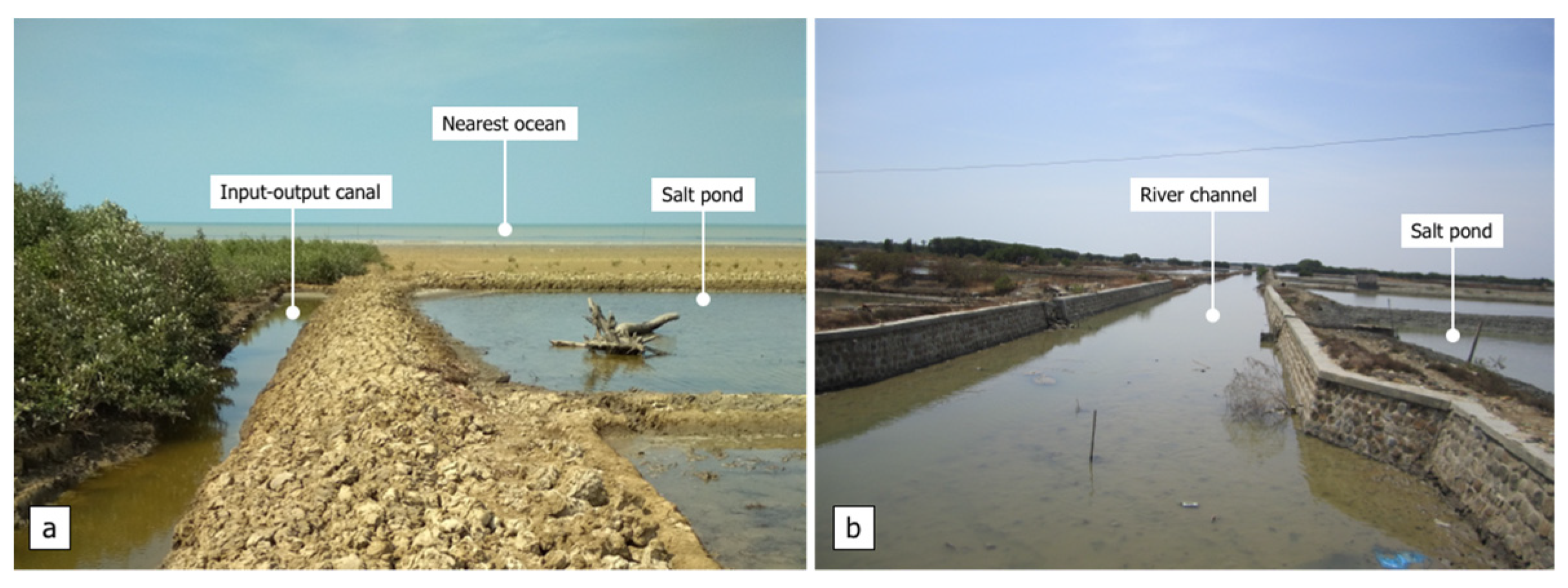
Figure 8.
The example sequence of a salt production pond at very high risk based on its physical condition and location (a) close to the shoreline and (b) close to channels (pictures taken by Nirwansyah in the Pangenan district).
Figure 8.
The example sequence of a salt production pond at very high risk based on its physical condition and location (a) close to the shoreline and (b) close to channels (pictures taken by Nirwansyah in the Pangenan district).


Table 1.
Scale of preference for the AHP model.
| Intensity Importance | Definition | Description |
|---|---|---|
| 1 |
|
|
| 3 |
|
|
| 5 |
|
|
| 7 |
|
|
| 9 |
|
|
| 2, 4, 6, 8 |
|
|
| Reciprocals |
|
|
Table 2.
Hazard and vulnerability components for the current study.
| Risk Components | Indicators | Functional Relation | Classes | Unit | Rank | Normalized Score |
|---|---|---|---|---|---|---|
| Hazard (H) | Depth (H1) | Direct | >150 100–150 50–100 15–50 <15 | cm | 1 2 3 4 5 | 0.33 0.27 0.20 0.13 0.07 |
| Duration (H2) | Direct | >5 2–5 <2 | day | 1 2 3 | 0.50 0.33 0.17 | |
| Timing (H3) | Conditional | Harvesting period Post-production period Construction period | 1 2 3 | 0.50 0.33 0.17 | ||
| Vulnerability (V) | Elevation (V1) | Inverse | <0.5 0.5–1 1–1.5 1.5–2 >2 | meter | 1 2 3 4 5 | 0.33 0.27 0.20 0.13 0.07 |
| Coastal slope (V2) | Inverse | <0.025 0.025–0.04 0.04–0.07 0.07–0.2 >0.2 | % | 1 2 3 4 5 | 0.33 0.27 0.20 0.13 0.07 | |
| Geology feature (V3) | Direct | Flood plain deposits Sand with silts and clay Mountain formation Younger volcanic | 1 2 3 4 | 0.40 0.30 0.20 0.10 | ||
| Soil type (V4) | Inverse | Alluvial Gleic Gleysol Cambisol Latosol | 1 2 3 4 | 0.40 0.30 0.20 0.10 | ||
| Distance to channel (V5) | Inverse | <200 200–400 400–600 600–800 >800 | meter | 1 2 3 4 5 | 0.33 0.27 0.20 0.13 0.07 | |
| Distance to shore (V6) | Inverse | <250 250–500 500–750 750–1000 >1000 | meter | 1 2 3 4 5 | 0.33 0.27 0.20 0.13 0.07 |
Table 3.
Random index (RI) matrix of the same dimension.
| Number of criteria | 2 | 3 | 4 | 5 | 6 | 7 | 8 | 9 | 10 | 11 |
| RI | 0.00 | 0.58 | 0.90 | 1.12 | 1.24 | 1.32 | 1.41 | 1.45 | 1.49 | 1.51 |
Source: Saaty, Vargas and Dellmann [102].
Table 4.
Parametric approach comparison using Pearson correlation test with input from simulated damage by the previous physical-based model * (loss is presented in thousand rupiahs).
Table 4.
Parametric approach comparison using Pearson correlation test with input from simulated damage by the previous physical-based model * (loss is presented in thousand rupiahs).
| 2016 Event | 2018 Event | |||
|---|---|---|---|---|
| Parametric | Physical-Based | Parametric | Physical-Based | |
| Minimum loss (on an individual parcel) | 0.00 | 0.00 | 0.00 | 0.00 |
| Maximum loss (on an individual parcel) | 13,287.28 | 13,322.72 | 2.491.73 | 2528.72 |
| Mean | 6500.68 | 6912.17 | 1240.87 | 1286.23 |
| Estimated total damage | 77,290,054 | 74,105,354 | 13,596,499 | 13,789,773 |
| Sample (n = 270 parcels) | ||||
| Pearson coefficient (r) | 0.81 | 0.84 | ||
| Type of correlation | Strongly positive | Strongly positive | ||
* The values were extracted from previous study by Nirwansyah and Braun [81].
Publisher’s Note: MDPI stays neutral with regard to jurisdictional claims in published maps and institutional affiliations. |
© 2021 by the authors. Licensee MDPI, Basel, Switzerland. This article is an open access article distributed under the terms and conditions of the Creative Commons Attribution (CC BY) license (https://creativecommons.org/licenses/by/4.0/).
Share and Cite
MDPI and ACS Style
Nirwansyah, A.W.; Braun, B. Tidal Flood Risk on Salt Farming: Evaluation of Post Events in the Northern Part of Java Using a Parametric Approach. Geosciences 2021, 11, 420. https://0-doi-org.brum.beds.ac.uk/10.3390/geosciences11100420
AMA Style
Nirwansyah AW, Braun B. Tidal Flood Risk on Salt Farming: Evaluation of Post Events in the Northern Part of Java Using a Parametric Approach. Geosciences. 2021; 11(10):420. https://0-doi-org.brum.beds.ac.uk/10.3390/geosciences11100420
Chicago/Turabian StyleNirwansyah, Anang Widhi, and Boris Braun. 2021. "Tidal Flood Risk on Salt Farming: Evaluation of Post Events in the Northern Part of Java Using a Parametric Approach" Geosciences 11, no. 10: 420. https://0-doi-org.brum.beds.ac.uk/10.3390/geosciences11100420
Note that from the first issue of 2016, this journal uses article numbers instead of page numbers. See further details here.