
Extreme Sea Surges, Tsunamis and Pluvial Flooding Events during the Last ~1000 Years in the Semi-Arid Wetland, Coquimbo Chile

 , , and
Abstract
:1. Introduction
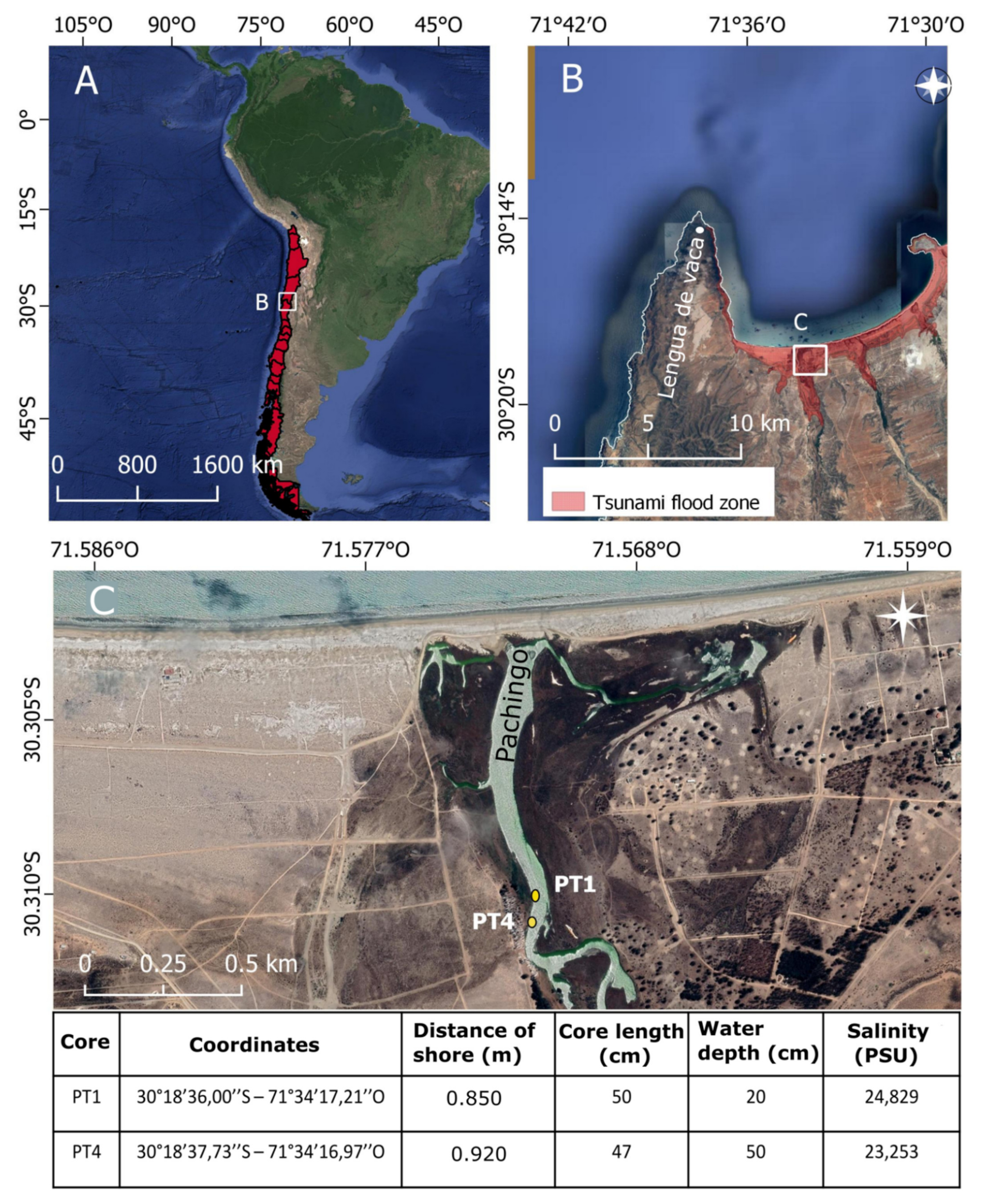
2. Study Area
3. Methodology
3.1. Lithology and Stratigraphy
3.2. Geochemical Characterization
3.3. Geochronology
3.4. Biogenic Components in the Sedimentary Records
3.5. SWAN Model
4. Results
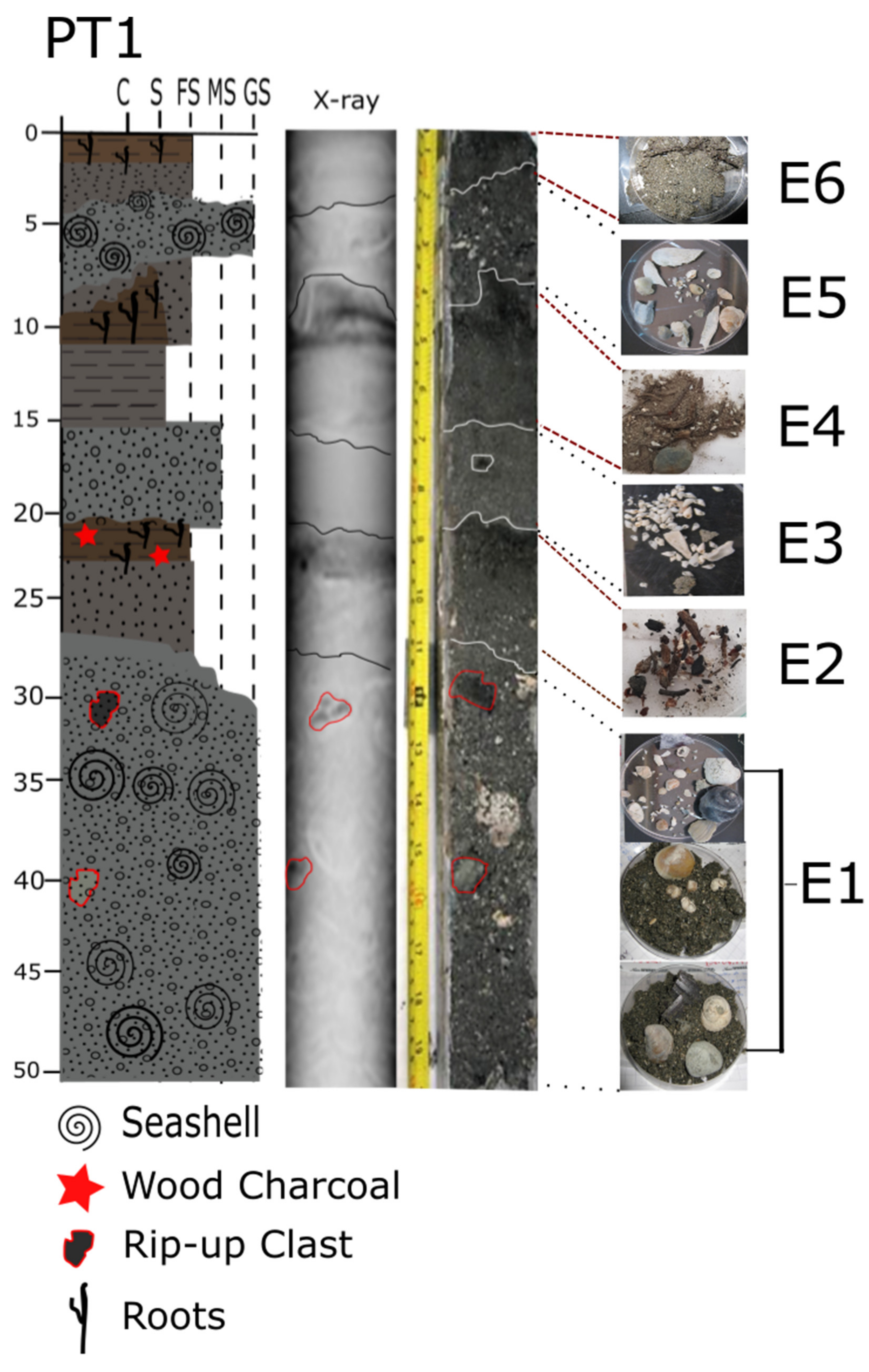
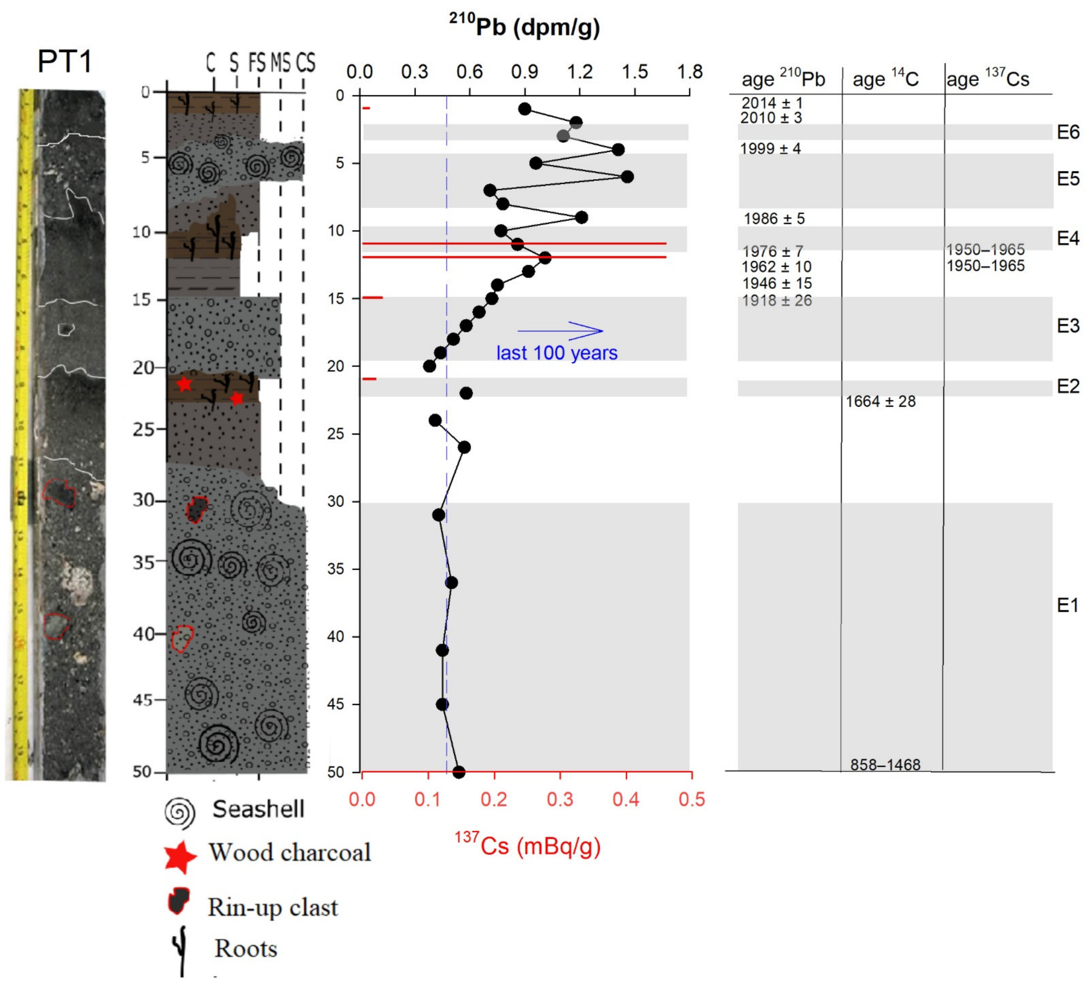
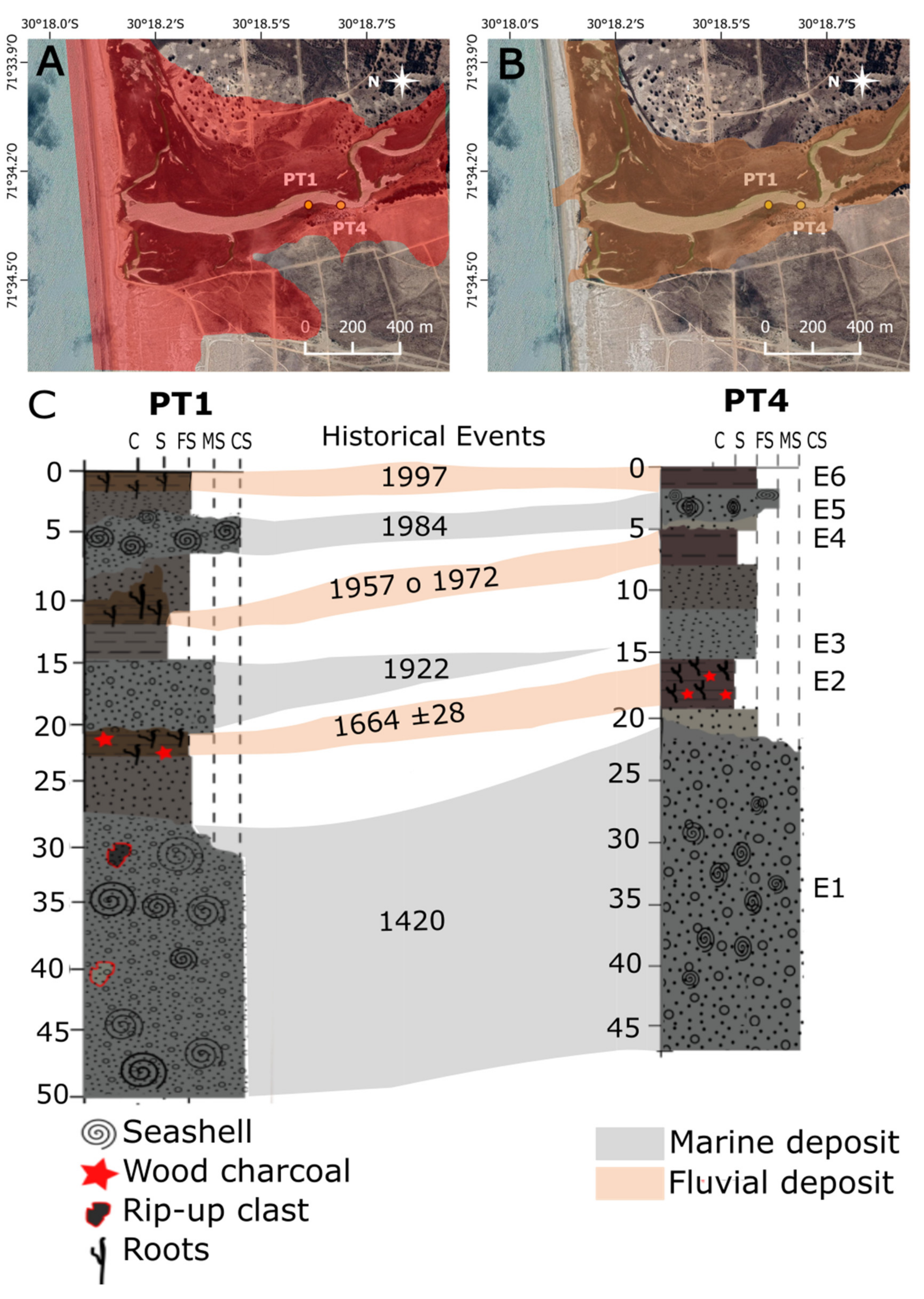
4.1. Lithostratigraphic Description
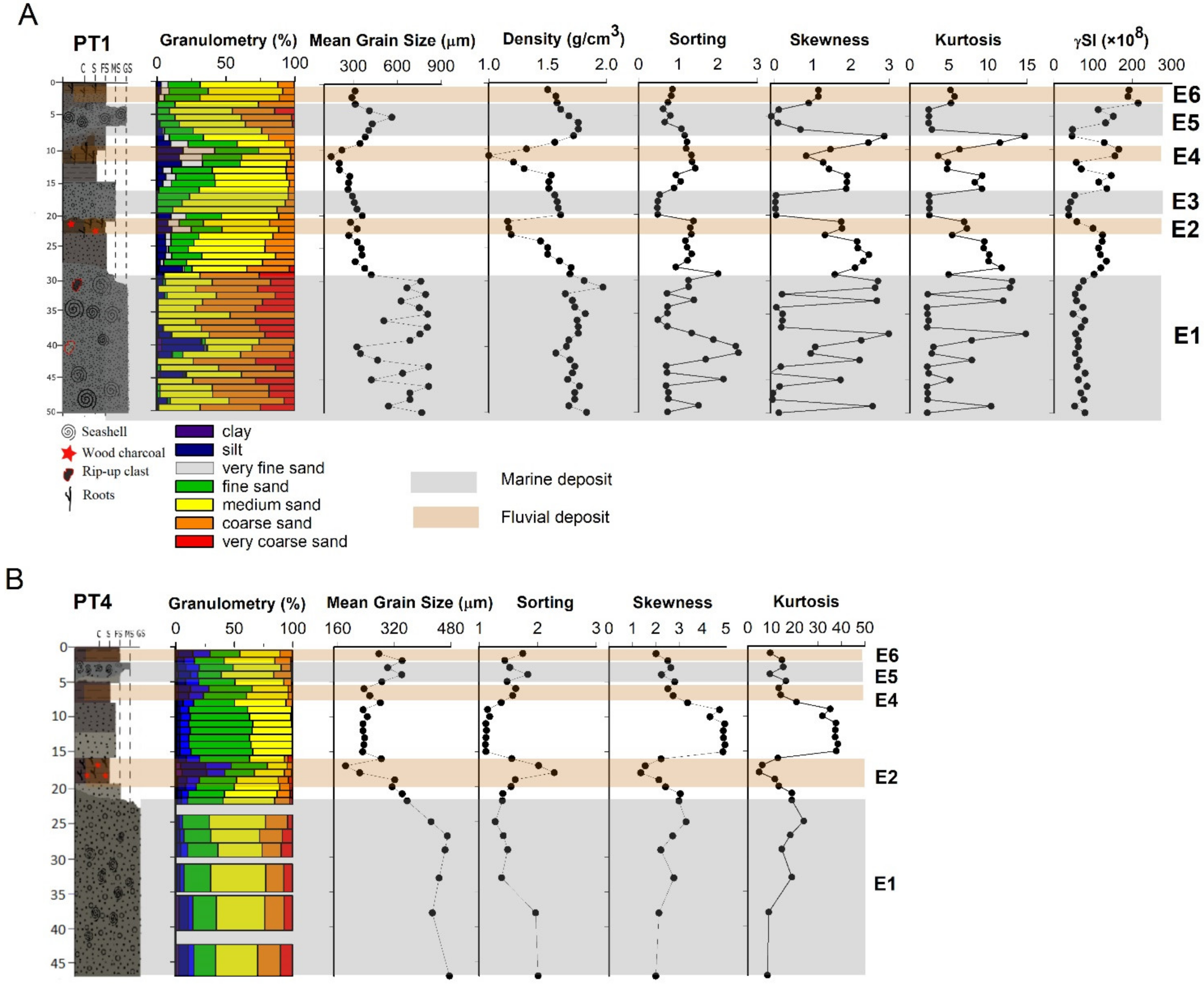
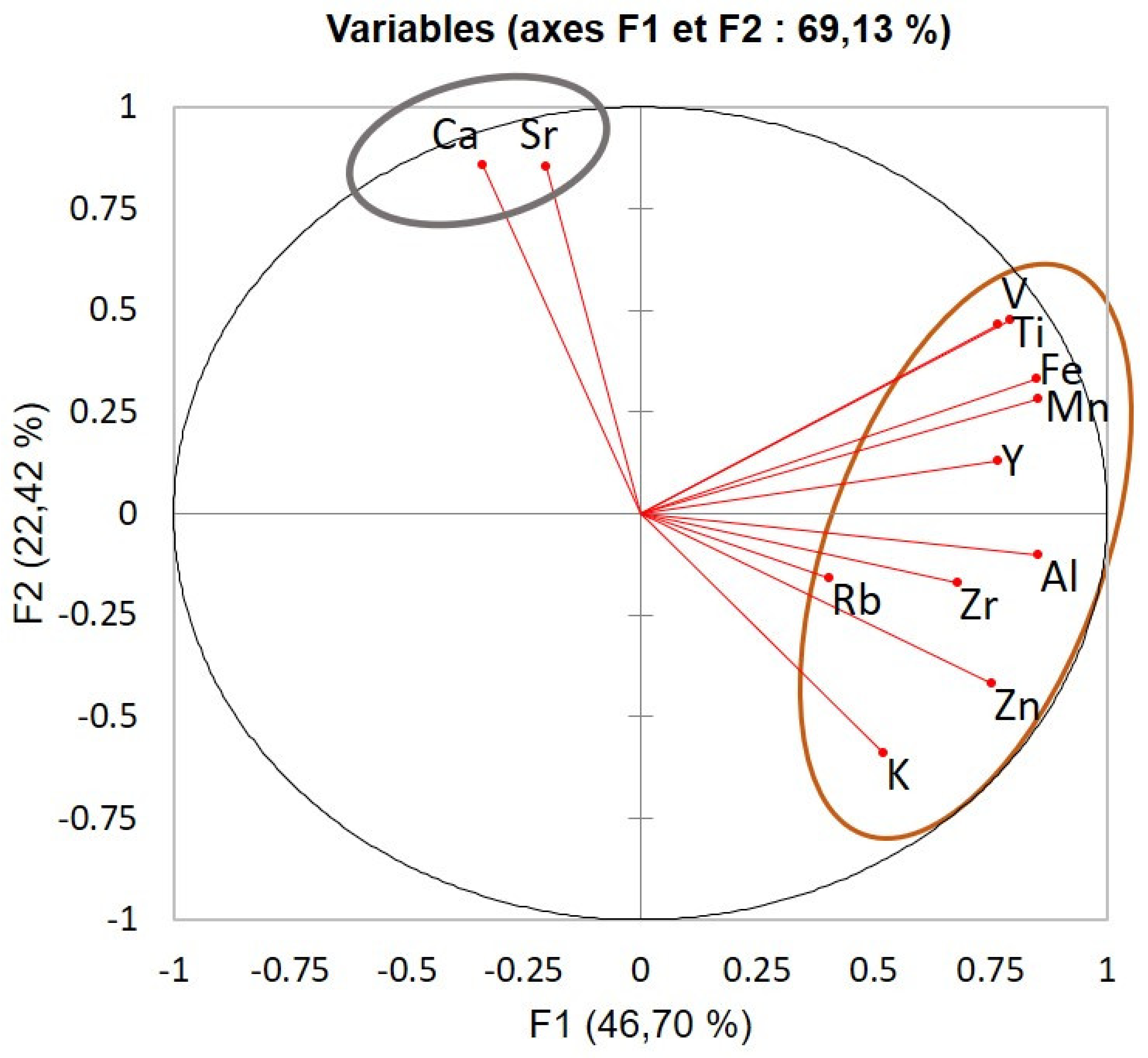
4.2. Geochemistry
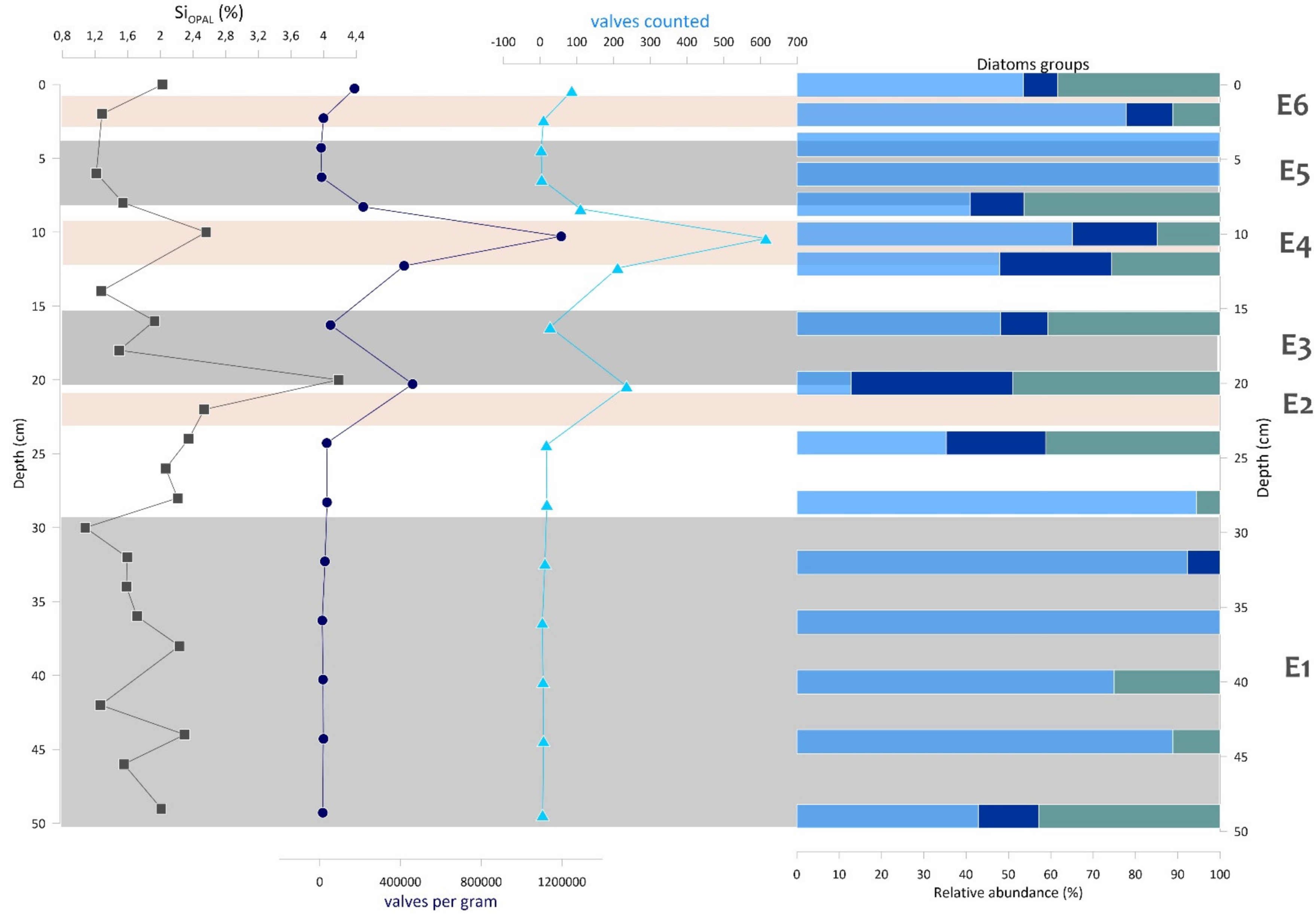
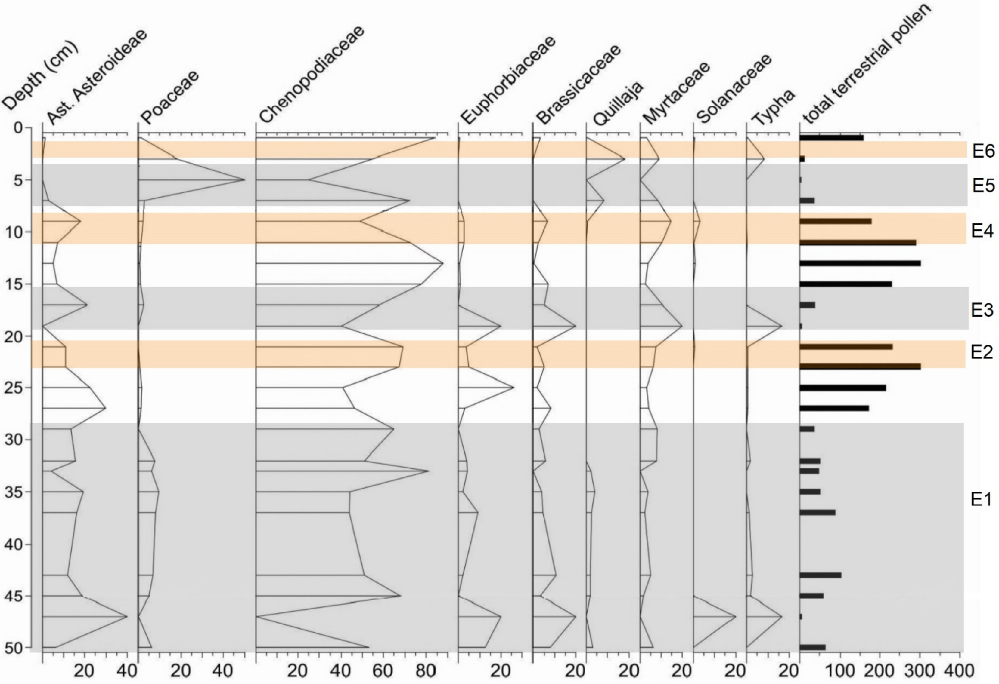
4.3. Biogenic Components
4.4. Marine and Flood Layer Identification
4.5. Geochronology
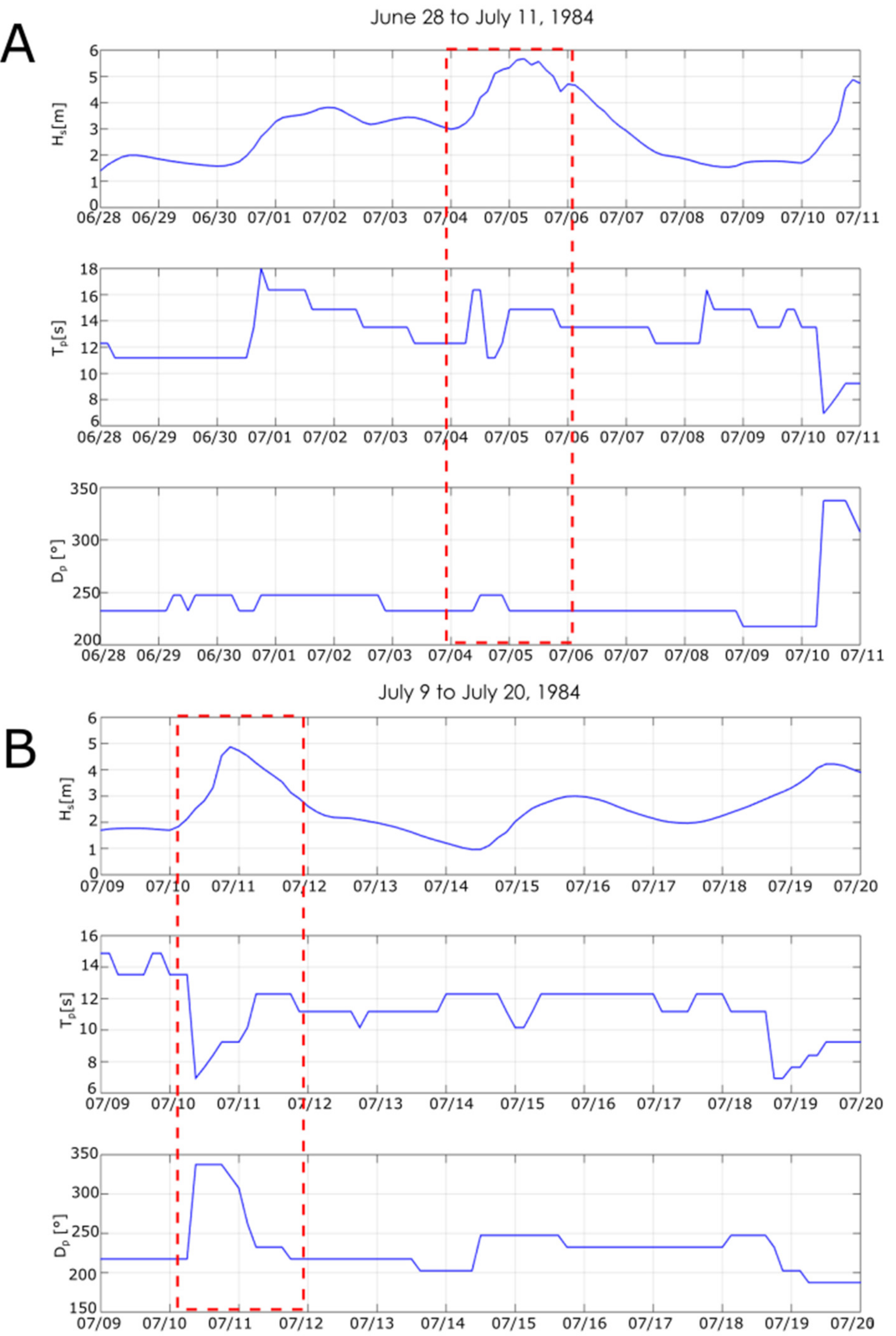
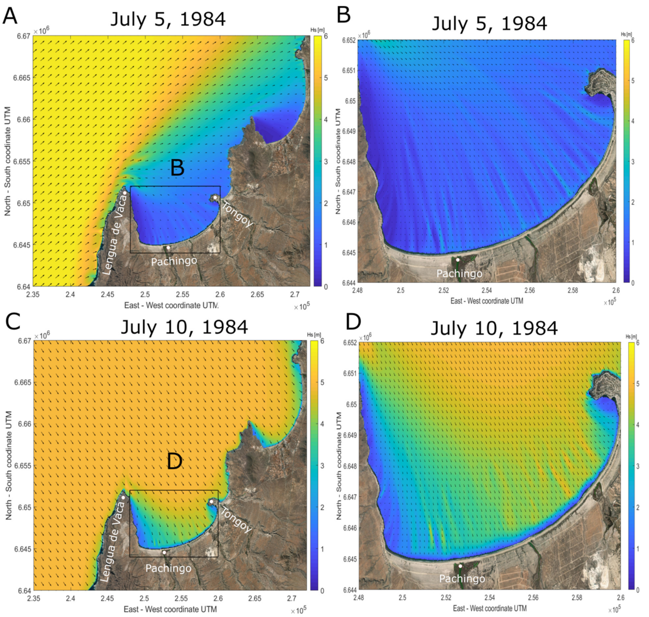
4.6. SWAN Model
5. Discussion
5.1. Extreme Events Identification
5.2. Reconstitution of Marine Submersion Deposits
5.3. Reconstitution of Flooding Associated Extreme Rain
6. Conclusions
Author Contributions
Funding
Institutional Review Board Statement
Informed Consent Statement
Data Availability Statement
Acknowledgments
Conflicts of Interest
Appendix A

| Freshwater (FW) | Marine (M) |
|---|---|
| Amphora copulata (Kützing) Schoeman & Archibald | Achnanthes brevipes C.Agardh |
| Cocconeis placentula var. lineata (Ehrenberg) | Grammatophora sp. 1 |
| Ctenophora pulchella (Ralfs ex Kützing) Williams & Round | Lyrella sp. 1 |
| Cyclotella meneghiniana (Kützing) | Lyrella sp. 2 |
| Diatoma vulgaris (Bory) | Surirella minuta Brebisson |
| Encyonema sp. 1 | Surirella striatula Turpin |
| Ephitemia sp. 2 | Rhaphoneis amphiceros (Ehrenberg) |
| Epithemia adnata (Kützing) Brébisson | |
| Gomphoneis sp. | |
| Gyrosigma acuminatum (Kützing) Rabenhorst 1853 | |
| Hantzschia amphioxys (Ehrenberg) Grunow | Brackish (BR) |
| Martyana schulzii (Brockmann) Snoeijs | Achnanthes submarina Hustedt |
| Navicula gregaria Donkin | Halamphora sp. |
| Navicula amphiceropsis Lange-Bertalot & Rumrich | Pleurosira laevis (Ehrenberg) Compère |
| Nitzschia palea (Kützing) W. Smith | Tabularia sp. |
| Pinnularia sp. 1 | Tryblionella sp. |
| Planothidium delicatulum (Kützing) Round & Bukhtiyarova | |
| Rhopalodia musculus (Kützing) Otto Müller | |
| Staurosirella martyi (Héribaud) Morales & Manoylov |
Appendix B

Appendix C

Appendix D

References
- Contreras-Lopez, M.; Winckler, P.; Sepulveda, I.; Andaur-Alvarez, A.; Cortés-Molina, F.; Guerrero, C.; Mizobe, C.; Igualt, F.; Wolfgang, B.; Beya, J.; et al. Field Survey of the 2015 Chile Tsunami with Emphasis on Coastal Wetland and Conservation Areas. Pure Appl. Geophys. 2016, 173, 349–367. [Google Scholar] [CrossRef]
- Barnhart, W.D.; Murray, J.R.; Briggs, R.W.; Gomez, F.; Miles, C.P.J.; Svarc, J.; Riquelme, S.; Stressler, B.J. Coseismic slip and early afterslip of the 2015 Illapel, Chile, earthquake: Implications for frictional heterogeneity and coastal uplift. J. Geophys. Res. Solid Earth 2016, 121, 6172–6191. [Google Scholar] [CrossRef] [Green Version]
- Ye, L.; Lay, T.; Kanamori, H.; Koper, K.D. Rapidly Estimated Seismic Source Parameters for the September 16 2015 Illapel, Chile M w 8.3 Earthquake. Pure Appl. Geophys. 2016, 173, 321–332. [Google Scholar] [CrossRef] [Green Version]
- Vigny, C.; Socquet, A.; Peyrat, S.; Ruegg, J.-C.; Métois, M.; Madariaga, R.; Morvan, R.; Lancieri, M.; Lacassin, R.; Campos, J.; et al. The 2010 Mw 8.8 Terremoto de megaempuje del Maule del centro de Chile, monitoreado por GPS. Ciencia 2011, 332, 417–421. [Google Scholar] [CrossRef] [Green Version]
- Delouis, B.; Nocquet, J.; Vallé, M. Slip distribution of the February 27, 2010 Mw = 8.8 Maule Earthquake, central Chile, from static and high-rate GPS, InSAR, and broadband teleseismic data. Geophys. Res. Lett. 2010, 37, L17305. [Google Scholar] [CrossRef] [Green Version]
- Campos, J.; Hatzfeld, D.; Madariaga, R.; Lopez, G.; Kausel, E.; Zollo, A.; Barrientos, S.; Lyon-Caen, H. The 1835 seismic gap in south central Chile. Phys. Earth Planet. Inter. 2002, 132, 177–195. [Google Scholar] [CrossRef]
- Izquierdo, T.; Abad, M.; Gómez, Y.; Gallardo, D.; Rodríguez-Vidal, J. The March 2015 catastrophic flood event and its impacts in the city of Copiapó (southern Atacama Desert). An integrated analysis to mitigate future mudflow derived damages. J. S. Am. Earth Sci. 2021, 105, 102975. [Google Scholar] [CrossRef]
- Bahlburg, H.; Nentwig, V.; Kreutzer, M. The September 16, 2015 Illapel tsunami, Chile—Sedimentology of tsunami deposits at the beaches of La Serena and Coquimbo. Mar. Geol. 2018, 396, 43–53. [Google Scholar] [CrossRef]
- Pérez, C.; Fiebig-Wittmaack, M.; Cepeda, J.; Pizarro-Araya, J. Desastres naturales y plagas en el Valle del rio Elqui. (Natural disasters and population outbreaks in the Elqui River valley). In Los Sistemas Naturales de la Cuenca del Rio Elqui (Región de Coquimbo, Chile): Vulnerabilidad y Cambio del Clima; Cepeda, P.J., Ed.; Ediciones Universidad de La Serena: La Serena, Chile, 2008; pp. 295–333. [Google Scholar]
- Ruiz, S.; Madariaga, R. Historical and Recent Large Megathrust Earthquakes in Chile. Tectonophysics 2018, 733, 37–56. [Google Scholar] [CrossRef]
- Soto, M.-V.; Märker, M.; Rodolfi, G.; Sepúlveda, S.A.; Cabello, M. Assessment of geomorphic processes affecting the paleo-landscape of Tongoy Bay, Coquimbo region, central Chile. Geogr. Fis. Din. Quat. 2014, 37, 51–66. [Google Scholar] [CrossRef]
- Métois, M.; Vigny, C.; Socquet, A.; Delorme, A.; Morvan, S.; Ortega, I.; Valderas- Bermejo, C.M. GPS-derived interseismic coupling on the subduction and seismic hazards in the Atacama region, Chile. Geophys. J. Int. 2013, 196, 644–655. [Google Scholar] [CrossRef] [Green Version]
- Udías, A.; Madariaga, R.; Buforn, E.; Muñoz, D.; Ros, M. The large Chilean historical earthquakes of 1647, 1657, 1730, and 1751 from contemporary documents. Bull. Seismol. Soc. Am. 2012, 102, 1639–1653. [Google Scholar] [CrossRef]
- Saillard, M.; Hall, S.R.; Audin, L.; Farber, D.L.; Herail, G.; Martinod, J.; Regard, V.; Finkel, R.C.; Bondoux, F. Non-steady longterm uplift rates and Pleistocene marine terrace development along the Andean margin of Chile (31 °S) inferred from 10Be dating. Earth Planet. Sci. Lett. 2009, 277, 50–63. [Google Scholar] [CrossRef]
- Lomnitz, C. Major earthquakes of Chile: A historical survey, 1535–1960. Seismol. Res. Lett. 2004, 75, 368–378. [Google Scholar] [CrossRef]
- Beck, S.; Barrientos, S.; Kausel, E.; Reyes, M. Source characteristics of historic earthquakes along the central Chile subduction zone. J. S. Am. Earth Sci. 1998, 11, 115–129. [Google Scholar] [CrossRef]
- DeMets, C.; Gordon, R.G.; Argus, D.F.; Stein, S. Effect of recent revisions to the geomagnetic reversal time scale on estimates of current plate motions. Geophys. Res. Lett. 1994, 21, 2191–2194. [Google Scholar] [CrossRef]
- Nishenko, S.P. Seismic potential for large and great interplate earthquakes along the Chilean and Southern Peruvian margins of South America: A quantitative reappraisal. J. Geophys. 1985, 90, 3589–3615. [Google Scholar] [CrossRef]
- Kellehier, J.A. Rupture zones of large South American earthquakes and some predictions. J. Geophys. Res. 1972, 11, 2087–2103. [Google Scholar] [CrossRef]
- Lomnitz, C. Major earthquakes and tsunamis in Chile during the period 1535 to 1955. Geol. Rundsch. 1970, 59, 938–960. [Google Scholar] [CrossRef]
- Kanamori, H.; Rivera, L.; Ye, L.; Lay, T.; Murotani, S.; Tsumura, K. New constraints on the 1922 Atacama, Chile, earthquake from Historical seismograms. Geophys. J. Int. 2019, 219, 645–661. [Google Scholar] [CrossRef] [Green Version]
- Carvajal, M.; Cisternas, M.; Gubler, A.; Catalán, P.A.; Winckler, P.; Wesson, R.L. Reexamination of the magnitudes for the 1906 and 1922 Chilean earthquakes using Japanese tsunami amplitudes: Implications for source depth constraints. J. Geophys. Res. Solid Earth 2017, 122, 4–17. [Google Scholar] [CrossRef]
- Dunbar, P.-K.; Lockridge, P.-A.; Whiteside, L.-S. Catalogue of Significant Earthquakes 2150 B.C.-1991 A.D.; World Data Center A for Solid Earth Geophysics Reports; U.S. Department of Commerce, NOAA, National Geophysical Data Center: Boulder, CO, USA, 1992; Volume SE-49, p. 320.
- Campos-Caba, R.V. Análisis de marejadas históricas y recientes en las costas de Chile. In Memoria de Título de Ingeniero Civil Oceánico; Facultad de Ingeniería, Universidad de Valparaíso: Valparaíso, Chile, 2016; p. 136. [Google Scholar]
- Campos-Caba, R.; Beyá, J.; Mena, M. Cuantificación de los Daños Históricos a Infraestructura Costera por Marejadas en las Costas de Chile. In Proceedings of the XXII Congreso Chileno de Ingeniería Hidráulica, SOCHID, Santiago, Chile, 21–23 October 2015; p. 14. [Google Scholar]
- Winckler, P.W.; Contreras, M.; Campos, R.C.; Beya, J.; Molina, M.M. El temporal del 8 de agosto de 2015 en las regiones de Valparaiso y Coquimbo, Chile Central. Latin Am. J. Aquat. Res. 2017, 45, 622–648. [Google Scholar] [CrossRef]
- Urrutia, H.; Lazcano, C.L. Catástrofes en Chile 1541–1992; Editorial La Noria: Santiago, Chile, 1993. [Google Scholar]
- Pérez, C. Cambio Climático: Vulnerabilidad, Adaptación y Rol Institucional. Estudio de Casos en el Valle de Elqui. Memoria para Optar al Título de Ingeniero Civil Ambiental; Facultad de Ingeniería, Universidad de La Serena: La Serena, Chile, 2005. [Google Scholar]
- Paris, R.; Fournier, J.; Poizot, E.; Etienne, S.; Morin, J.; Lavigne, F.; Wassmer, P. Boulder and fine sediment transport and deposition by the 2004 tsunami in Lhok Nga (western Banda Aceh, Sumatra, Indonesia): A coupled offshore–onshore model. Mar. Geol. 2010, 268, 43–54. [Google Scholar] [CrossRef]
- Paris, R.; Wassmer, P.; Sartohadi, J.; Lavigne, F.; Barthomeuf, B.; Desgages, E.; Grancher, D.; Baumert, P.; Vautier, F.; Brunstein, D. Tsunamis as geomorphic crises: Lessons from the 26 December 2004 tsunami in Lhok Nga, west Banda Aceh (Sumatra, Indonesia). Geomorphology 2009, 104, 59–72. [Google Scholar] [CrossRef]
- Liu, K.; Fearn, M.L. Lake-sediment record of Late Holocene hurricane activities from coastal Alabama. Geology 1993, 21, 793–796. [Google Scholar] [CrossRef]
- May, S.; Pint, A.; Rixhon, G.; Kelletat, D.; Wennrich, V.; Brückner, H. Holocene coastal stratigraphy, coastal changes and potential palaeoseismological implications inferred from geo-archives in Central Chile (29–32 °S). Z. Für Geomorphol. Suppl. Issues 2013, 57, 201–228. [Google Scholar] [CrossRef] [Green Version]
- Day, J.W.; Christian, R.R.; Boesch, D.M.; Yáñez-Arancibia, A.; Morris, J.; Twilley, R.; Naylor, L.; Schaffner, L.; Stevenson, C. Consecuencias del Cambio Climático en la Ecogeomorfología de los Humedales Costeros. Estuarios Costas 2008, 31, 477–491. [Google Scholar] [CrossRef]
- Long, A.J.; Waller, M.P.; Stupples, P. Driving mechanisms of coastal change: Peat compaction and the destruction of late Holocene coastal wetlands. Mar. Geol. 2006, 25, 63–84. [Google Scholar] [CrossRef] [Green Version]
- Cundy, A.B.; Kortekaas, S.; Dewez, T.; Stewart, I.S.; Collins, P.E.F.; Croudace, I.W.; Maroukian, H.; Papanastassiou, D.; Gaki-Papanastassiou, P.; Pavlopoulos, K.; et al. Coastal wetlands as recorders of earthquake subsidence in the Aegean: A case study of the 1894 Gulf of Atalantiearthquakes, central Greece. Mar. Geol. 2000, 170, 3–26. [Google Scholar] [CrossRef]
- Parish, F.; Sirin, A.; Charman, D.; Joosten, H.; Minaeva, T.; Silvius, M. Assessment on Pleatlands, Biodiversity and Climate Change; Global Environment Center: Kuala Lumpur, Malaysia; Wentlands International: Wageningen, The Netherlands, 2008. [Google Scholar]
- McCaffrey, R.; Thomson, J. A Record of the Accumulation of Sediment and Trace Metals in a Connecticut Salr Marsh; Elsevier: Amsterdam, The Netherlands, 1980; Volume 22, pp. 165–236. [Google Scholar]
- Woodruff, J.D.; Donnelly, J.P.; Emanuel, K.; Lane, P. Assessing sedimentary records of paleohurricane activity using modeled hurricane climatology. Geochem. Geophys. Geosyst. 2008, 9, 9. [Google Scholar] [CrossRef]
- Dezileau, L.; Sabatier, P.; Blanchemanche, P.; Joly, B.; Swingedouw, D.; Cassou, C.; Castaings, J.; Martinez, P.; Von Grafenstein, U. Intense storm activity during the Little Ice Age on the French Mediterranean coast. Palaeogeogr. Palaeoclimatol. Palaeoecol. 2011, 299, 289–297. [Google Scholar] [CrossRef]
- DePaolis, J.M.; Dura, T.; MacInnes, B.; Lisa, L.E.; Cisternas, M.; Carvajal, M.; Tang, H.; Fritz, H.M.; Mizobe, C.; Wesson, R.L.; et al. Stratigraphic evidence of two historical tsunamis on the semi-arid coast of north-central Chile. Quat. Sci. Rev. 2021, 226, 1070252. [Google Scholar] [CrossRef]
- Khalfaoui, O.; Dezileau, L.; Degeai, J.; Snoussi, M. Reconstruction of past marine submersion events (storms and tsunamis) on the North Atlantic coast of Morocco. Nat. Hazards Earth Syst. Sci. Discuss. 2019, 130, 11–14. [Google Scholar] [CrossRef]
- Degeai, J.-P.; Devillers, B.; Dezileau, L.; Oueslati, H.; Bony, G. Major storm periods and climate forcing in the Western Mediterranean during the Late Holocene. Quat. Sci. Rev. 2015, 129, 37–56. [Google Scholar] [CrossRef]
- Raji, O.; Dezileau, L.; Von Grafenstein, U.; Niazi, S.; Snoussi, M.; Martinez, P. Extreme sea events during the last millennium in the northeast of Morocco. Nat. Hazards Earth Syst. Sci. 2015, 15, 1533–1543. [Google Scholar] [CrossRef] [Green Version]
- Shennan, S.; Downey, S.; Timpson, A.; Edinborough, K.; Colledge, S.; Kerig, T.; Manning, K.; Thomas, M.G. Regional population collapse followed initial agriculture booms in mid-Holocene Europe. Nat. Commun. 2013, 4, 2486. [Google Scholar] [CrossRef] [Green Version]
- Sabatier, P.; Dezileau, L.; Condomines, M.; Briqueu, L.; Colin, C.; Bouchette, F.; Le Duff, M.; Blanchemanche, P. Reconstruction of paleostorm events in a coastal lagoon (Hérault, south of France). Mar. Geol. 2008, 251, 224–232. [Google Scholar] [CrossRef]
- Nanayama, A.C.; Tatavarti, R.; Shinu, N.; Subeer, A. Tsunami of 26 December 2004 on the southwest coast of India: Post-tsunami geomorphic and sediment characteristics. Mar. Geol. 2007, 242, 155–168. [Google Scholar]
- Scileppi, E.; Donnelly, J.P. Sedimentary evidence of hurricane strikes in western Long Island, NY. Geochem. Geophys. Geosyst. 2007, 8, Q06011. [Google Scholar] [CrossRef]
- Donnelly, J.P.; Cleary, P.; Newby, P.; Ettinger, R. Coupling Instrumental and Geological Records of Sea-Level Change: Evidence from southern New England of an increase in the rate of sea-level rise in the late 19th century. Geophys. Res. Lett. 2004, 31, L05203. [Google Scholar] [CrossRef] [Green Version]
- Dezileau, L.; Lehu, R.; Lallemand, S.; Hsu, S.-K.; Babonneau, N.; Ratzov, G.; Lin, A.; Dominguez, S. Historical Reconstruction of Submarine Earthquakes Using Pb-210, Cs-137, and Am-241 Turbidite Chronology and Radiocarbon Reservoir Age Estimation off East Taiwan. Radiocarbon 2016, 58, 25–36. [Google Scholar] [CrossRef]
- Dezileau, L.; Bordelais, S.; Condomines, M.; Bouchette, F.; Briqueu, L. Evolution des Lagunes du Golfe d’Aigues-Mortes à Partir de l’Étude de Carottes Sédimentaires Courtes (Étude Géochronologique, Sédimentologique et Géochimique des Sédiments Récents); Publications ASF: Paris, France, 2015; Volume 51, p. 91. [Google Scholar]
- Webster, P.J.; Holland, G.J.; Curry, J.A.; Chang, H.R. Change in tropicalcyclone number, duration, and intensity in a warming environment. Science 2000, 309, 1844–1846. [Google Scholar] [CrossRef] [Green Version]
- Collins, E.S.; Scott, D.B.; Gayes, P.T. Hurricane records on the South Carolina coast: Can they be detected in the sediment record? Quat. Int. 1999, 56, 15–26. [Google Scholar] [CrossRef]
- Paskoff, R. Contribuciones recientes al conocimiento del cuaternario marino del centro y norte de Chile. Revista de Geografía Norte Grande 1999, 26, 43–575. [Google Scholar]
- Herm, D.; Paskoff, R. Vorschlag zur Gliederung des marinen Quart&s en Nord- und Mittel-Chile. Neues Jahrb. Geol. Palontología Montashefte 1967, 10, 577–588. [Google Scholar]
- Ota, Y.; Paskoff, R. Holocene deposits on the coast of north-central Chile: Radiocarbon ages and implications for coastal changes. Rev. Geol. Chile 1993, 20, 25–32. [Google Scholar] [CrossRef]
- Ortega, C.; Vargas, G.; Rutllant, J.; Jackson, D.; Méndez, C. Major hydrological regime change along the semiaridwestern coast of South America during the Early Holocene. Quat. Res. 2012, 78, 513–527. [Google Scholar] [CrossRef]
- Rutllant, J.; Montecino, V. Multiscale upwelling forcing cycles and biological response off northcentral Chile. Ciclos multiescala en el forzamiento de la surgencia y respuesta biológica en el centro-norte de Chile. Rev. Chil. Hist. Nat. 2002, 75, 217–231. [Google Scholar] [CrossRef] [Green Version]
- Rutllant, J.; Fuenzalida, H. Synoptic aspects of the central Chile rainfall variability associated with the Southern Oscillation. Int. J. Clim. 1991, 11, 63–76. [Google Scholar] [CrossRef]
- Soto, M.-V.; Arriagada-Gonzalez, J.; Cabello-Espinola, M. The Accretional Beach Ridge System of Tongoy Bay: An Example of a Regressive Barrier Developed in the Semiarid Region of Chile. Recent Adv. Petrochem. Sci. (RAPSCI) 2018, 4, 1–8. [Google Scholar] [CrossRef]
- Lagos, S.G. Caracterización Geomorfológica y Dinámica Costera de Bahías del Semiárido de Chile; Universidad de Chile: Santiago, Chile, 2013; p. 87. [Google Scholar]
- Figueroa, R.; Suárez, M.L.; Asunción, A.; Ruiz, V.; Vidal-Abarca, M. Wetlands ecological characterization of Central Chile semi-dry area. Gayana 2009, 73, 76–94. [Google Scholar]
- Niemeyer, H. Hoyas Hidrográficas de Chile Cuarta Región. Obtenido de DGA (General Directorate of Waters). 1980. Available online: https://snia.mop.gob.cl/sad/CUH2886v4.pdf (accessed on 20 October 2021).
- Downing, S.M.; Baranowski, R.A.; Grosso, L.J.; Norcini, J.J. Item type and cognitive ability measured: The validity evidence for multiple true–false items in medical specialty certification. Appl. Meas. Educ. 1995, 8, 89–199. [Google Scholar] [CrossRef]
- Montecinos, A.; Aceituno, P. Seasonality of the ENSO-Related Rainfall Variability in Central Chile and Associated Circulation Anomalies. J. Clim. 2002, 16, 281–296. [Google Scholar] [CrossRef] [Green Version]
- Hogg, A.G.; Heaton, T.J.; Hua, Q.; Palmer, J.G.; Turney, C.S.M.; Southon, J.; Bayliss, A.; Blackwe, P.G.; Boswijk, G.; Bronk-Ramsey, C.; et al. SHCal20 Southern Hemisphere calibration, 0-55,000 years cal BP. Radiocarbon 2020, 62, 759–778. [Google Scholar] [CrossRef]
- Heaton, T.; Köhler, P.; Butzin, M.; Bard, E.; Reimer, R.; Austin, W.; Skinner, L. Marine20—The Marine Radiocarbon Age Calibration Curve (0–55,000 cal BP). Radiocarbon 2020, 62, 779–820. [Google Scholar] [CrossRef]
- Marshall, J.D.; Brooks, J.R.; Lajtha, K. Sources of Variation in the Stable Isotopic Composition of Plants. In Stable Isotopes in Ecology and Environmental Science; Michener, R., Lajtha, K., Eds.; John Wiley & Sons: Hoboken, NJ, USA, 2007. [Google Scholar] [CrossRef]
- Khan, N.S.; Vane, C.H.; Horton, B.P. Stable carbon isotope and C/N geochemstry of coastal wetland sediments as a sea-level indicator. Handb. Sea-Level Res. 2015, 1, 295–311. [Google Scholar]
- Carrasco-Puga, G.; Díaz, F.P.; Soto, D.C.; Hernández-Castro, C.; Contreras-López, O.; Maldonado, A.; Latorre, C.; Gutiérrez, R.A. Revealing hidden plant diversity in arid environments. Ecography 2021, 44, 98–111. [Google Scholar] [CrossRef]
- Jara, I.; Maldonado, A.; Porras, M.E. Late Holocene dynamics of the south American summer monsoon: New insights from the Andes of northern Chile (21° S). Quat. Sci. Rev. 2020, 246, 106533. [Google Scholar] [CrossRef]
- Hong, I.; Dura, T.; Ely, L.L.; Horton, B.P.; Nelson, A.R.; Cisternas, M.; Nikitina, D.; Wesson, R.L. A 600-year-year-long stratigraphic record of tsunamis in south-central Chile. Holocene 2016, 27, 1–13. [Google Scholar] [CrossRef] [Green Version]
- De Porras, M.E.; Maldonado, A.; Zamora-Allendes, A.; Latorre, C. Calibrating the pollen signal in modern rodent middens from northern Chile to improve the interpretation of the late Quaternary midden record. Quat. Res. 2015, 84, 301–311. [Google Scholar] [CrossRef]
- Sawai, Y.; Fujii, Y.; Fujiwara, O.; Kamataki, T.; Komatsubara, J.; Okamura, Y.; Satake, K.; Shishikura, M. Marine incursión of the past 1500 years and evidence of tsunamis at suijin-numa, a coastal lake facing the Japan Trench. Holocene 2008, 18, 517–528. [Google Scholar] [CrossRef]
- Maldonado, A.; Betancourt, J.L.; Latorre, C.; Villagran, C. Pollen analyses from a 50 000-yr rodent midden series in the southern Atacama Desert (25°30′ S). J. Quat. Sci. 2005, 20, 493–507. [Google Scholar] [CrossRef]
- Dura, T.; Cisternas, M.; Horton, B.; Ely, L.; Nelson, A.; Wesson, R.; Pilarczyk, J. Coastal evidence for Holocene subduction-zone earthquakes and tsunamis in central Chile. Quat. Sci. Rev. 2015, 113, 93–111. [Google Scholar] [CrossRef]
- Rivera, R. Guide for References and Distribution for the Class Bacillariophyceae in Chile between 18°28′ S and 58 °S; J. Cramer: Summit, NJ, USA, 1983. [Google Scholar]
- Rebolledo, L.; Lange, C.B.; Figueroa, D.; Pantoja, S.; Muñoz, P.; Castro, R. 20th century fluctuations in the abundance of siliceous microorganisms preserved in the sediments of the Puyuhuapi Channel (44 °S), Chile. Rev. Chil. Hist. Nat. 2005, 78, 469–488. [Google Scholar] [CrossRef] [Green Version]
- Vos, P.C.; de Wolf, H. Methodological aspects of paleo-ecological diatom research in coastal areas of the Netherlands. Geol. Mijnb. 1988, 67, 31–40. [Google Scholar]
- Faegri, K.; Iversen, J. Textbook of Pollen Analysis. Blackwell Scientific Publication, 4th ed.; John Wiley and Sons: Chichester, UK, 1989. [Google Scholar]
- Holthuijsen, L. Olas en Aguas Oceánicas y Costeras; Cambridge University Press: Cambridge, UK, 2007. [Google Scholar] [CrossRef]
- Winckler, P. Introducción al Modelado de Procesos Costeros, 1st ed.; Universidad de Valparaíso: Valparaíso, Chile, 2018. [Google Scholar]
- Beyá, J.; Alvarez, M.; Gallardo, A.; Hidalgo, H.; Aguirre, C.; Valdivia, J.; Parra, C.; Méndez, F.; Contreras, F.; Winckler, P.; et al. Atlas de Oleaje de Chile; Escuela de Ingeniería Civil Oceánica, Universidad de Valparaíso: Valparaíso, Chile, 2016; p. 169. [Google Scholar]
- Arnaud, F.; Lignier, V.; Revel, M.; Desmet, M.; Beck, C.; Pourchet, M.; Charlet, F.; Trentesaux, A.; Tribovillard, N. Flood and earthquake disturbance of 210Pb geochronology Lake Anterne, NW Alps. Terra Nova 2002, 14, 225–232. [Google Scholar] [CrossRef]
- Robbins, J.A.; Edgington, D.N. Determination of recent sedimentation rates in Lake Michigan using Pb-210 and Cs-137. Geochim. Cosmochim. Acta 1979, 39, 285–304. [Google Scholar] [CrossRef] [Green Version]
- Carré, M.; Jacksonb, D.; Maldonado, A.; Chase, B.M.; Sachs, J.P. Variability of 14C reservoir age and air—Sea flux of CO2 in the Peru–Chile upwelling region during the past 12,000 years. Quat. Res. 2016, 85, 87–93. [Google Scholar] [CrossRef]
- Ortega, C.; Vargas, G.; Rojas, M.; Rutllant, J.; Muñoz, P.; Lange, C.B.; Pantoja, S.; Dezileau, L.; Ortlieb, L. Extreme ENSO-driver torrential rainfalls at the southern Edge of the Atacama Desert during the Late Holocene and their projection into the 21th century. Glob. Planet. Change 2019, 175, 226–237. [Google Scholar] [CrossRef]
- Muñoz, P.; Rebolledo, L.; Dezileau, L.; Maldonado, A.; Mayr, C.; Cárdenas, P.; Lange, C.B.; Lalangui, K.; Sánchez, G.; Salamanca, M.; et al. Reconstructing past variations in environmental conditions and paleoproductivity over the last ~8000 years off north-central Chile (30° S). Biogeociencias 2020, 22, 5763–5785. [Google Scholar] [CrossRef]
- Lambeck, K.; Bard, E. Sea-level change along the French Mediterranean coast for the past 30,000 years—Earth Planet. Sci. Lett. 2000, 175, 203–222. [Google Scholar]
- Takashi, I.; Kazuhisa, G.; Yusuke, Y.; Yosuke, M.; Chikako, S.; Keita, T. Reducing the age range of tsunami deposits by 14C dating of rip-up clasts. Sediment. Geol. 2018, 364, 334–341. [Google Scholar] [CrossRef]
- Sakuna-Schwartz, D.; Feldens, P.; Schwarzer, K.; Khokiattiwong, S.; Stattegger, K. Internal structure of event layers preserved on the Andaman Sea continental shelf, Thailand: Tsunami vs. storm and flash-flood deposits. Nat. Hazards Earth Syst. Sci. 2015, 15, 1181–1199. [Google Scholar] [CrossRef] [Green Version]
- Switzer, A.D.; Jones, B.G. Large-scale washover sedimentation in a freshwater lagoon from the southeast Australian coast: Sea-level change, tsunami or exceptionally large storm? Holocene 2008, 5, 787–803. [Google Scholar] [CrossRef]
- Morton, R.A.; Gelfenbaum, G.; Jaffe, B.E. Physical criteria for distinguishing sandy tsunami and storm deposits using modern examples. Sediment. Geol. 2007, 200, 184–207. [Google Scholar] [CrossRef]
- Lomnitz, C. Development in Geotectonics #5, Global Tectonics and Earthquake Risk; Elsevier Scientific Publishing Co.: Amsterdam, The Netherlands, 1974. [Google Scholar]
- Soloviev, S.L.; Go, C.N. A Catalogue of Tsunamis on the Western Shore of the Pacific Ocean [Dates Include 173–1968]; Academy of Sciences of the USSR, Nauka Publishing House: Moscow, Russia, 1974; p. 439. [Google Scholar]
- Imamura, A. Topographical Changes Accompanying Earthquake or Volcanic Eruptions; Publications of the Earthquake Investigation Committee in Foreign Languages: Tokyo, Japan, 1930; Volume 35, pp. 16–38. [Google Scholar]
- Abad, M.; Izquierdo, T.; Cáceres, M.; Bernárdez, E.; Vidal, J. Coastal boulder deposit as evidence of an ocean-wide prehistoric tsunami originated on the Atacama Desert coast (Northern Chile). Sedimentology 2020, 67, 1505–1528. [Google Scholar] [CrossRef]
- Nentwig, V.; Bahlburg, H.; Górecka, E.; Huber, B.; Bellanova, P.; Witkowski, A.; Encinas, A. Multiproxy analysis of tsunami deposits—The Tirúa example, central Chile. Geosphere 2018, 14, 1067–1086. [Google Scholar] [CrossRef] [Green Version]
- Sakate, K.; Heidarzadeh, M.; Quiroz, M.; Cienfuegos, R. History and features of trans-oceanic tsunamis and implications for paleo-tsunami studies. Earth-Sci. Rev. 2020, 202, 103–112. [Google Scholar]
- Lockridge, P.A. Tsunamis in Peru-Chile. In World Data Center a for Solid Earth Geophysics; National Geophysical Data Center: Boulder, CO, USA, 1985; Report SE-39; 97p. [Google Scholar]
- Ceresis: Centro Regional de Sismología para América del Sur. Catálogo de Terremotos para América del Sur; 1985, 12 Lima, Perú. Available online: http://www.ceresis.org/ (accessed on 20 October 2021).
- Urbina, X.; Gorigoitía, N.; Cisternas, M. Aportes a la historia sísmica de Chile: El caso del gran terremoto de 1730. Anu. Estud. Am. 2016, 73, 657–687. (In Spanish) [Google Scholar] [CrossRef] [Green Version]
- NCEI/WDS: National Geophysical Data Center/World Data Service: Global Historical Tsunami Database; NOAA National Centers for Environmental Information: Stennis Space Center, MI, USA, 2020. [CrossRef]
- Nakamura, S. An Analysis of the 1985 Chilean Tsunami. Mar. Geod. 1992, 15, 277–281. [Google Scholar] [CrossRef]
- Maturana, J.; Bello, M.; Manley, M. Antecedentes Históricos y Descripción del Fenómeno El Niño, Oscilación del Sur. History and Description of “El Niño, Southern Oscillation” Phenomenon; SHOA—Servicio Hidrográfico y Oceanográfico de la Armada de Chile, Departamento de Oceanografía: Valparaíso, Chile, 2004. [Google Scholar]
- Quinn, W.; Neal, V.T.; Mayolo, S.E.A. El Niño ocurrences over the past four and half centuries. J. Geophys. Res. 1987, 92, 14449–14461. [Google Scholar] [CrossRef]
- Koutavas, A.; de Menocal, P.B.; Olive, G.C.; Lynch-Stieglitz, J. Mid-Holocene El Niño–Southern Oscillation (ENSO) attenuation revealed by individual foraminifera in eastern tropical Pacific sediments. Geology 2006, 34, 993–996. [Google Scholar] [CrossRef]
- Morales, M.S.; Cook, E.R.; Barichivich, J.; Christie, D.A.; Villalba, R.; LeQuesne, C.; Srur, A.M.; Ferrero, M.E.; González-Reyes, A.; Couvreux, F.; et al. Six hundred years of South American tree rings reveal an increase in severe hydroclimatic events since mid-20th century. Proc. Natl. Acad. Sci. USA 2020, 117, 16816–16823. [Google Scholar] [CrossRef] [PubMed]
- Ferrada, A.; Christie, D.A.; Muñoz, F.; González, A.; Garreaud, R.D.; Bustos, S. Explorador del Atlas de Sequías de Sudamérica; Centro de Cienciencia del Clima y la Resiliencia (CR)2: Santiago, Chile, 2021. [Google Scholar]
- Rein, B.; Lückge, A.; Reinhardt, L.; Sirocko, F.; Wolf, A.; Dullo, W.C. Variabilidad de El Niño frente a Perú durante los últimos 20.000 años. Paleoceanografía 2005, 20, PA4003. [Google Scholar] [CrossRef]
- Morales, M.; Duncan, A.C.; Neukom, R.; Rojas, F.; Villalba, R. Variabilidad Hidroclimática en el Sur del Altiplano: Pasado, Presente y Futuro. La Puna Argentina Naturaleza y Cultura, Serie Conservación de la Naturaleza 24: La Puna Argentina: Naturaleza y Cultura, Fundación Miguel Lillo; Fundación Miguel Lillo: Tucumán, Argentina, 2018; ISBN 978-950-668-032-9. [Google Scholar]
- Prieto, M.D. ENSO signals in South America: Rains and floods in the Paraná River region during colonial times. Clim. Chang. 2007, 83, 39–54. [Google Scholar] [CrossRef]
- Cepeda, P.J. (Ed.) Los Sistemas Naturales de la Cuenca del Rio Elqui (Región de Coquimbo, Chile): Vulnerabilidad y Cambio del Clima; Ediciones Universidad de La Serena: La Serena, Chile, 2008. [Google Scholar]


| Fraction Modern | 14C Age | Age Calib | |||||||||
|---|---|---|---|---|---|---|---|---|---|---|---|
| ID | Material | Section | Lab Code | pMC | 1σ Error | BP | 1σ Error | BC/AD | BC/AD | BC/AD | BC/AD |
| Core | cm | DirectAMS | 210Pb | ΔR 625 ± 46 a | ΔR 165 ± 107 b | ΔR 442 c | |||||
| PT1 | Shell | 1 | D-AMS 009072 | 94.27 | 0.29 | 474 | 25 | 2010 | invalid age | invalid age | invalid age |
| PT1 | Shell | 8 | D-AMS 009060 | 87.62 | 0.26 | 1062 * | 24 | 1986 | invalid age | 1468–1700 | 1832–1950 |
| PT1 | Shell | 23 | D-AMS 009061 | 76.14 | 0.22 | 2190 * | 23 | - | 901–1072 | 403–658 | 729–871 |
| PT1 | Wood charcoal | 24 | D-AMS 013087 | 96.68 | 0.34 | 271 | 28 | - | 1640–1671 | 1640–1671 | 1640–1671 |
| PT1 | Shell | 36 | D-AMS 009063 | 74.59 | 0.27 | 2355 * | 30 | - | 726–902 | 199–491 | 580–700 |
| PT1 | Shell | 49 | D-AMS 009064 | 80.56 | 0.28 | 1736 * | 28 | - | 1336–1468 | 858–1129 | 1205–1324 |
| Date | Hs [m] | Tp [s] | Dp [°] |
|---|---|---|---|
| 5 July 1984 | 5.67 | 14.8 | 232.5 |
| 10 July 1984 | 4.87 | 9.2 | 322.5 |
| ID | ID | Section | Sorting | Contact | Munsell Color Scale | Other Characteristics | |
|---|---|---|---|---|---|---|---|
| Core | Unit | cm | Upper | Basal | |||
| PT1 | E1 | 30–50 | Moderately sorted Very poorly sorted * | Sharp | - | 2.5Y 4/1 | High content of gravel, angular fragments of seashell, seashell and two rip-up clasts (30 and 40 cm) |
| PT1 | E2 | 20–22 | Poorly sorted | Relatively sharp | Sharp | 2.5Y 2.5/1 | High content of roots, wood charcoal and estuarine shell |
| PT1 | E3 | 16–19 | Well sorted | Relatively sharp | Relatively sharp | 2.5Y 4/1 | High content of gravel and fragments of angular seashell |
| PT1 | E4 | 10–12 | Poorly sorted | Sharp | Slightly sharp | 2.5Y 2.5/1 | High content of roots, round gravel, wood charcoal and estuarine shell |
| PT1 | E5 | 4–8 | Moderately well sorted | Relatively sharp | Sharp | 2.5Y 4/1 | High content of gravel and seashell fragments |
| PT1 | E6 | 2–3 | Moderately sorted | gradational | Relatively sharp | 2.5Y 3/1 | High content of roots and estuarine shell |
| PT4 | E1 | 22–47 | Poorly sorted | Sharp | - | 2.5Y 4/1 | High content of gravel, angular fragments of seashell and seashell |
| PT4 | E2 | 17–20 | Very poorly sorted | Relatively sharp | Sharp | 2.5Y 2.5/1 | High content of roots, wood charcoal and estuarine shell |
| PT4 | E4 | 6–8 | Poorly sorted | Slightly sharp | Slightly sharp | 2.5Y 2.5/1 | High content of roots and estuarine shell |
| PT4 | E5 | 3–5 | Poorly sorted | Relatively sharp | Sharp | 2.5Y 4/1 | High content of gravel, angular fragments of seashell and seashell |
| PT4 | E6 | 1–2 | Poorly sorted | Gradational | Relatively sharp | 2.5Y 2.5/1 | Presence of gravel, angular fragments of seashell, seashell and fish bones |
Publisher’s Note: MDPI stays neutral with regard to jurisdictional claims in published maps and institutional affiliations. |
© 2022 by the authors. Licensee MDPI, Basel, Switzerland. This article is an open access article distributed under the terms and conditions of the Creative Commons Attribution (CC BY) license (https://creativecommons.org/licenses/by/4.0/).
Share and Cite
Araya, K.; Muñoz, P.; Dezileau, L.; Maldonado, A.; Campos-Caba, R.; Rebolledo, L.; Cardenas, P.; Salamanca, M. Extreme Sea Surges, Tsunamis and Pluvial Flooding Events during the Last ~1000 Years in the Semi-Arid Wetland, Coquimbo Chile. Geosciences 2022, 12, 135. https://0-doi-org.brum.beds.ac.uk/10.3390/geosciences12030135
Araya K, Muñoz P, Dezileau L, Maldonado A, Campos-Caba R, Rebolledo L, Cardenas P, Salamanca M. Extreme Sea Surges, Tsunamis and Pluvial Flooding Events during the Last ~1000 Years in the Semi-Arid Wetland, Coquimbo Chile. Geosciences. 2022; 12(3):135. https://0-doi-org.brum.beds.ac.uk/10.3390/geosciences12030135
Chicago/Turabian StyleAraya, Karen, Práxedes Muñoz, Laurent Dezileau, Antonio Maldonado, Rodrigo Campos-Caba, Lorena Rebolledo, Paola Cardenas, and Marco Salamanca. 2022. "Extreme Sea Surges, Tsunamis and Pluvial Flooding Events during the Last ~1000 Years in the Semi-Arid Wetland, Coquimbo Chile" Geosciences 12, no. 3: 135. https://0-doi-org.brum.beds.ac.uk/10.3390/geosciences12030135