
GEOENT: A Toolbox for Calculating Directional Geological Entropy


1
Dipartimento di Scienze della Terra, Università degli Studi di Milano, 20133 Milan, Italy
2
British Geological Survey, Keyworth, Nottingham NG12 5GG, UK
*
Author to whom correspondence should be addressed.
Geosciences 2022, 12(5), 206; https://0-doi-org.brum.beds.ac.uk/10.3390/geosciences12050206
Submission received: 28 February 2022
/
Revised: 5 May 2022
/
Accepted: 10 May 2022
/
Published: 12 May 2022
(This article belongs to the Section Hydrogeology)
Abstract
:Geological entropy is based on Shannon information entropy and measures order in the structure of a spatial random variable. Metrics have been defined to quantify geological entropy in multidimensional (2D and 3D) heterogeneous systems, for instance, porous and fractured geological media. This study introduces GEOENT, a toolbox that can efficiently be used to calculate geological entropy metrics for any kind of input-gridded field. Additionally, the definition of geological entropy metrics is updated to consider anisotropy in the structure of the heterogeneous system. Directional entrograms provide more accurate descriptions of spatial order over different Cartesian directions. This study presents the development of the geological entropy metrics, a description of the toolbox, and examples of its applications in different datasets, including 2D and 3D gridded fields, representing a variety of heterogeneous environments at different scales, from pore-scale microtomography (μCT) images to aquifer analogues.
Keywords:
heterogeneity; entropy; mathematical code; subsurface; spatial mapping; information theory1. Introduction
Shannon information entropy [1] is a widely adopted concept to calculate the average level of uncertainty (or surprise) of a random variable. The concept has been used in virtually all fields of research and types of application, including genome biology [2], linguistics [3], finance [4], and cryptography [5]. Shannon information entropy can be used to obtain quantitative information regarding the complexity and chaos of disordered multidimensional systems [6,7,8,9,10,11,12,13].
Bianchi and Pedretti [14,15] developed the concept of ‘geological entropy’ to quantify the spatial order of geological environments. Functions (e.g., ‘entrograms’) and metrics (e.g., ‘entropic scale’) based on Shannon information entropy were derived to quantify the spatial order of multidimensional (2D and 3D) heterogeneous porous and fractured media [16,17,18,19]. Bianchi and Pedretti [14,15] showed that geological entropy metrics describing the spatial order of heterogeneous aquifers can explain certain characteristics of the behaviour of solutes migrating in these aquifers. In particular, solute transport is known to be very sensitive to the spatial organization of the hydraulic properties of the geological media, such as the presence of highly permeable coarse-grained in alluvial materials or fractures in fractured media [20,21,22]. Bianchi and Pedretti [14,15] demonstrated that the relative entropy and the entropic scale (all defined in detail in the following sections) are well correlated to metrics that reflect solute transport in heterogeneous aquifers, such as the BTC skewness.
Despite these previous studies presenting the mathematical background of geological entropy, at present, no codes, scripts, or toolboxes have been released to readily calculate geological entropy metrics. Additionally, geological entropy metrics have thus far been considered only statistically isotropic structures, while random spatial fields can present anisotropy when certain statistical properties such as the spatial disorder vary over spatial directions. In alluvial aquifers, for instance, anisotropy may result directly from depositional processes [23,24]. Therefore, directionality should always be considered in geological entropy analysis, and metrics such as ‘directional entrograms’ should be used to better describe the spatial order of a random field over different directions.
In this study, we introduce GEOENT, a versatile and efficient MATLAB®-coded toolbox that can be used to compute geological entropy. GEOENT calculates directional entrograms and corresponding metrics for 2D or 3D gridded continuous or categorical datasets. In this manuscript, we present the development of the toolbox and its applications using different examples of datasets. We first revise the key aspects of the directional geological entropy algorithm. Then, we explain the toolbox structure, including the main script and the algorithm to compute the directional entrograms. We finally apply GEOENT to 2D and 3D gridded images representing different heterogeneous environments at different scales.
2. Materials and Methods
2.1. Mathematical Definition of Directional Entrograms
For a categorical random variable, as in the case of the hydrofacies of an alluvial aquifer, the Shannon information entropy (H) evaluates the marginal probabilities of occurrence of each category within subdomains of the entire field [14,15]. Higher H values indicate higher disorder, meaning that all the categories have similar marginal probabilities within a subdomain, while lower H values indicate that there is a predominant category. The equations for the calculation of H are reported in Appendix A.
In our first study in which the concept was introduced [14], H was computed over a small-scale, fixed-size, isotropic 2D or 3D block. The approach was subsequently extended [15], and H was computed over increasing spatial scales, starting from an initial isotropic block of random values and growing until reaching the desired size within the limit of the size of the entire dataset. This resulted in the definition of an entrogram, which graphically describes the change in over growing scales, similarly to the variogram typically used in geostatistical analyses.
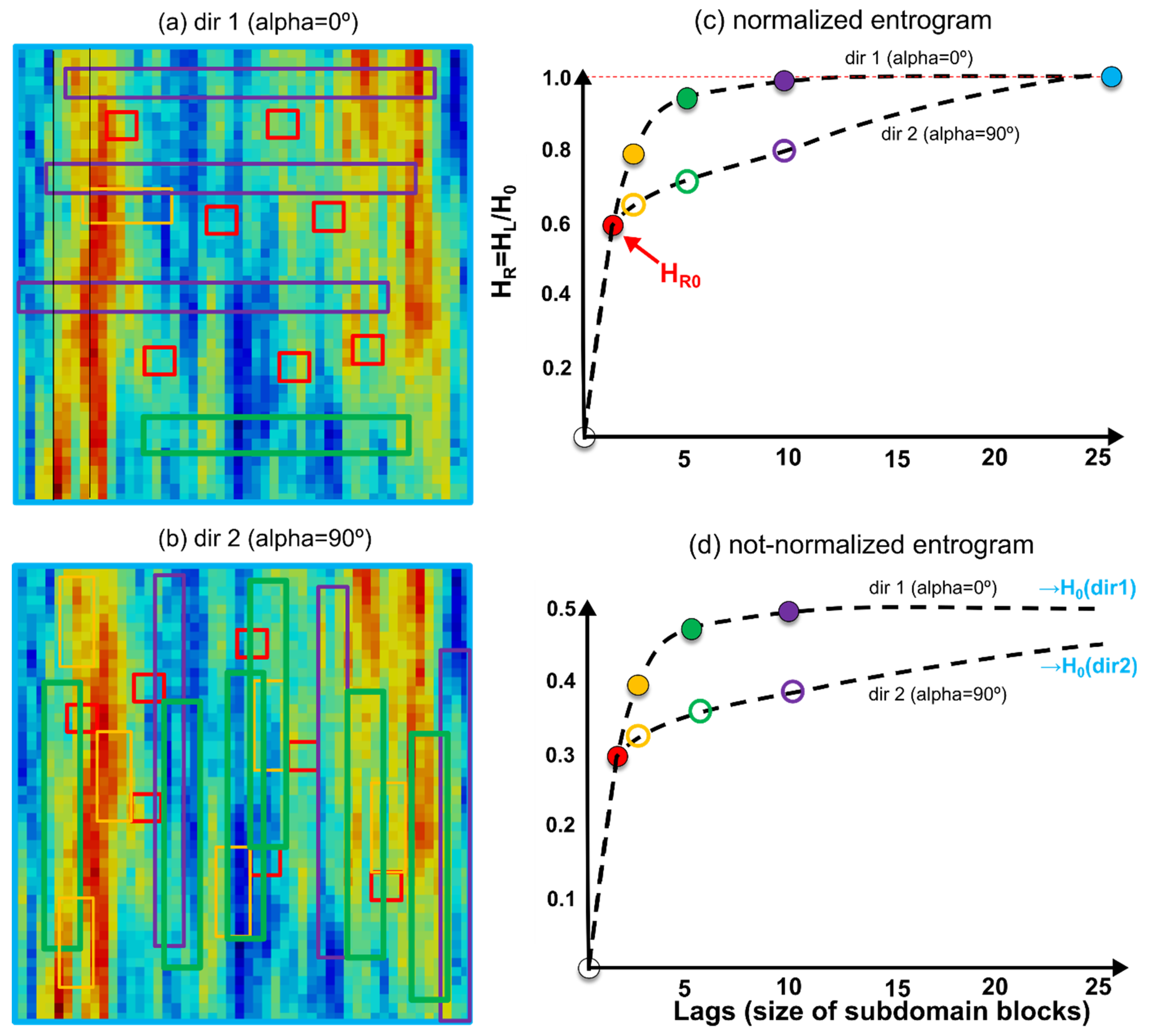
The algorithm to compute directional entrograms is conceptually depicted in Figure 1 for a 2D random system, although the approach is identical for a 3D system. A subdomain with dimension is first defined, where are the unit vectors = (1, 0, 0), (1, 0, 0), (0, 0, 1), and and are the scalar components of , which also correspond to the ‘entrogram lag’. For a 2D system, = 1. Starting from an initial random position in the space, the first ‘local entropy’ () is computed as
where is the number of categories for a discrete random variable or the total number of bins used to discretise the probability density function of a continuous variable, and is the local proportion of or marginal probabilities of occurrence of the categories within the subdomain (e.g., in geology, the ‘volumetric fractions’ of the facies within the searching box). In GEOENT, the shape of the searching box at the smallest scale is a cube (a square in 2D application) of size = unit, where the unit is the grid size of the input dataset. The local entropy is normalised to obtain the relative entropy (, such that
where defines the entropy calculated for the entire system. The process is repeated times each time for a different, randomly selected starting point, keeping the same subdomain size. An average relative entropy is then computed as
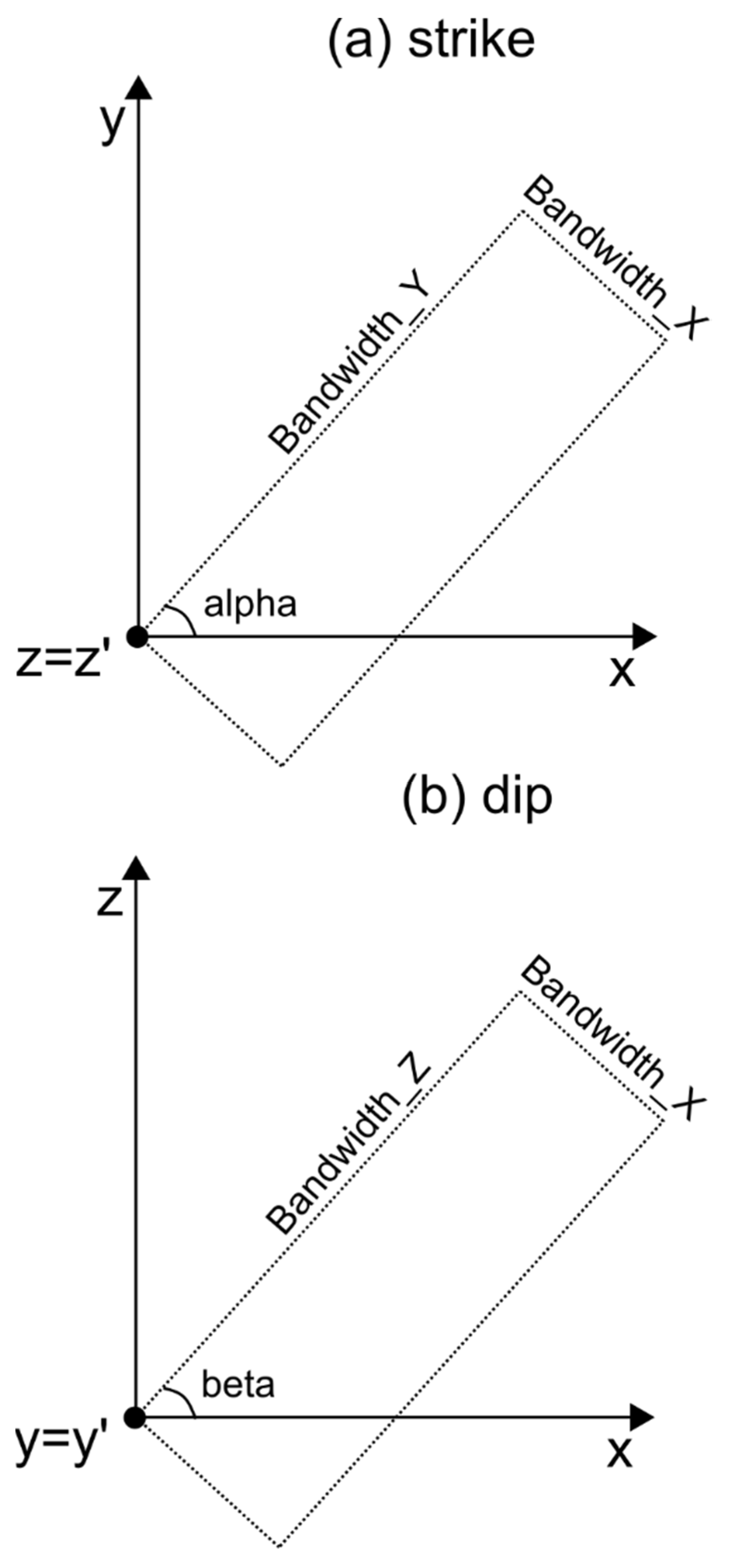
The operation (Equations (1)–(3)) is repeated for larger subdomains and plotted against by increasing lags to form the entrogram curve. A subdomain can grow identically in each direction () to obtain a regular searching box, resulting in ‘isotropic’ entrograms and corresponding metrics (defined below) or being elongated in a specific direction to obtain an irregular searching box, resulting in one or more ‘anisotropic’ or ‘directional’ entrograms. Regarding the term ‘bandwidth’, we define the size of the domain in each direction (‘dir’) and ‘NDIR’ as the number of directions evaluated via a GEOENT analysis. In the example shown in Figure 1, we considered two different main directions (NDIR = 2), according to which the searching box increases parallel to the horizontal and vertical axes, respectively, of the analysed 2D dataset. In the plane, angle defines the direction along which the bandwidth of the searching box is rotated around z (‘the strike’). For 3D systems, angle defines the directions along which the bandwidth of the searching box is rotated around y (‘the dip’). The angles and size that define the directional shape of the searching box are graphically shown in Figure 2.
The normalization in Equation (2) is such that, for any direction, . The more ordered a system is over larger spatial scales, the longer it takes for the entrograms to reach . An entropic scale () can be calculated to quantify the spatial order of a random field [15]. This scale is defined as
such that systems characterised by larger tend to present higher persistency of patterns of spatial association of certain categories and, therefore, spatial order in their spatial structure.
The shape of the directional entrograms can be very different depending on the direction along which the searching box is oriented. While remains the same, the spatial order along specific directions can change depending on the statistical anisotropy of the random field of interest. The more ordered a variable is along a specific direction, the longer a directional entrogram will take to reach the asymptotic value. Thus, the entrogram scale must be computed for each direction. In the case of rectangular 2D or hexahedral 3D domains, the searching box can grow more in one direction than in the others. Therefore, it is useful to normalise by the size of the searching box in a specific direction. A normalised entropic scale, , is thus calculated such that
where ) is the maximum bandwidth of the searching box along the ith direction.
It is finally possible that the global entropy computed over the entire dataset, , may not reflect the fact that a statistically anisotropic system remains, on average, more ordered over a specific direction. In other words, the global entropy over a specific direction may be lower than the global entropy of the system, simply because the disorder is more likely to occur in other directions. Thus, we can compute a final metric, , which is the local entropy calculated for each direction at large lags. The metric corresponds to the limit at which the entropy will tend if the system is analysed exclusively along a specific (i) direction.
2.2. Implementation in GEOENT
GEOENT is a MATLAB®-coded toolbox that calculates the directional entrograms and geological entropy metrics using the algorithm described in the previous section. GEOENT can be easily adapted to work in other MATLAB-like environments, such as GNU OCTAVE. GEOENT is available in a GitHub repository (https://github.com/hydrogeolab/GEOENT; accessed on 12 January 2022), in which it is distributed under GNU Lesser General Public License v3.0. The repository contains several zipped files with the main scripts and routines, as well as multiple examples (including those described in this manuscript), to run GEOENT with different kinds of input datasets.
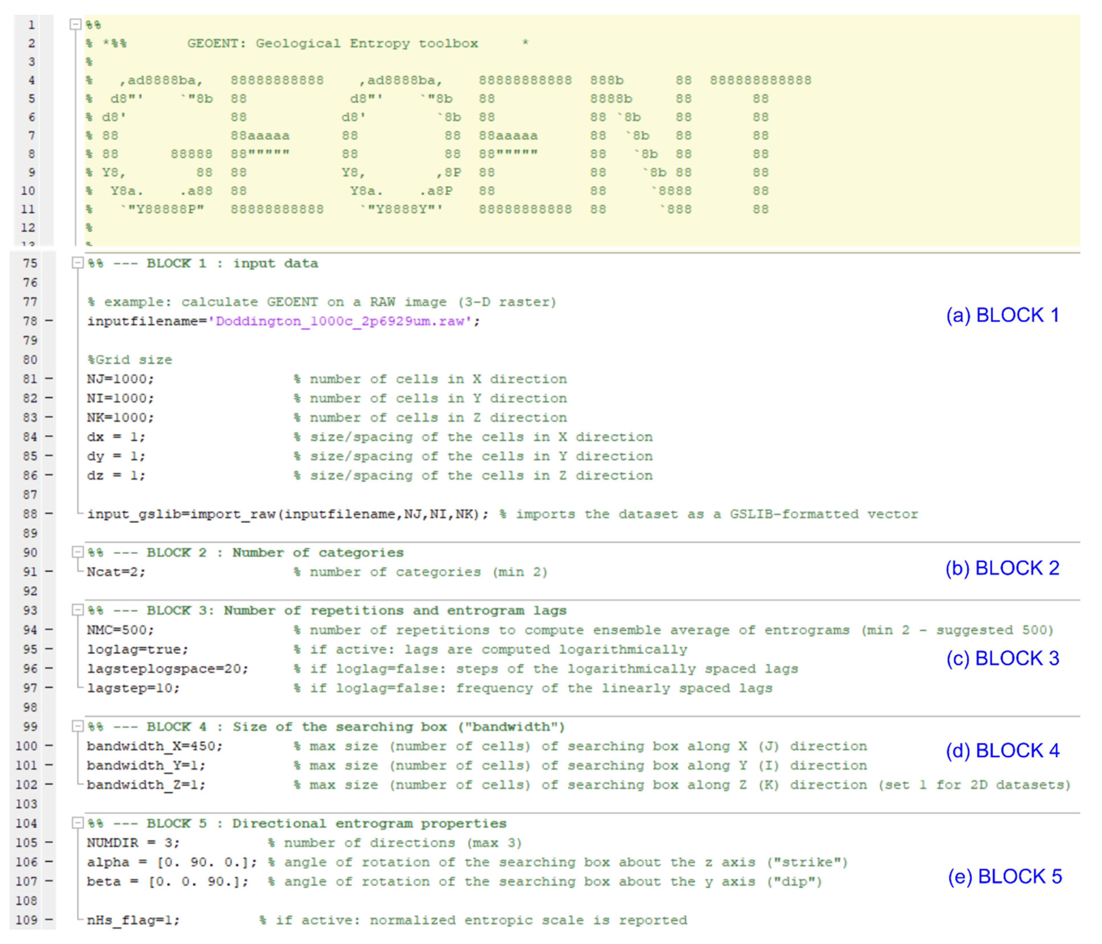
The main files are ‘GEOENT.m’, the script with which the user sets up the dataset-specific information and runs the calculation, and ‘Entrogram.m’, the main routine to compute the directional entrograms. The script ‘GEOENT.m’ (Figure 3) is structured in seven ‘blocks’, of which the first five (Block 1 to Block 5) contain user inputs for setting up the calculation, and the remaining two blocks contain instructions for calling the algorithm (Block 6) and plotting the results (Block 7).
In Block 1, the user defines the dataset size and resolution. This routine works with Cartesian grids, for which the user defines the grid dimensions in the X, Y, and Z directions (called, respectively, NJ, NI, and NK) and the grid or voxel size (dx, dy, and dz). Depending on the type of input dataset, the user may require additional scripts to import the dataset into the specific format required by GEOENT. Examples of such files can be located in the subfolders containing the provided testing analyses. In the standard version of GEOENT, the input dataset should be introduced using a GSLIB [25] formatting style (http://www.gslib.com/gslib_help/format.html; accessed on 12 May 2022), based on which a multidimensional dataset is converted into a one-dimensional vector. A GSLIB vector is formatted such that
where loc identifies the position of a node in the vector, and ix, iy, and iz are, respectively, the node coordinates in x, y, and z. For instance, a 10 × 5 × 2 dataset is converted into a 200-node vector.
In Block 2, the user defines the number of categories (NCat), into which the input dataset is discretised. The minimum number is Ncat = 2, which results in a binary distribution. In Block 3, the first set of parameters controlling the searching algorithms for the entrogram calculations is specified. The user defines the number of times (NMC) that the searching box changes the location to compute the local entrograms. For NMC = 2 (the minimum number), the algorithm computes the local entropy based on the relative entropy of two specific locations in which the searching box is centred. To obtain statically stable results, it is convenient to set up a larger number of repetitions. It is suggested that NCM ≥ 500, although the user can perform a sensitivity analysis around this number to obtain the best number as a trade-off between computational time and smoothness/stability of the computed entrograms.
In Block 4, the user indicates the directional bandwidths, which define the size of the searching box in the three Cartesian directions. To conduct anisotropic analysis, the user should input identical bandwidths for each direction. In Block 5, the user defines the number of directions (NDIR) and the angles of rotation—alpha and beta. The first rotation is about the vertical z axis (i.e., the strike), and the second is about the y axis (i.e., the dip).
The calculation of the entrograms is performed in Block 6, where the script Entrogram.m is called. For each direction (nd = 1:NDIR), the number of processed lags appears in the MATLAB ‘Command Window’, informing the user about the speed of the calculation process. GEOENT calculates the global Shannon entropy of this dataset (), the relative entropy (), the entrogram for each direction, and the corresponding non-normalised and normalised entropy scales ( and ).
The resulting outputs are graphically processed using the commands defined in Block 7, and ASCII output files containing the entrograms in the different directions are created. Figures of the global-entropy-normalised and non-normalised entrograms are generated and saved as .fig files, which also contain the computed entrograms metrics. The user is given the option to save the results in a binary MATLAB .mat file and the figures in .png by uncommenting the related code lines.
3. Application of GEOENT to Representative Datasets
3.1. Illustrative Example
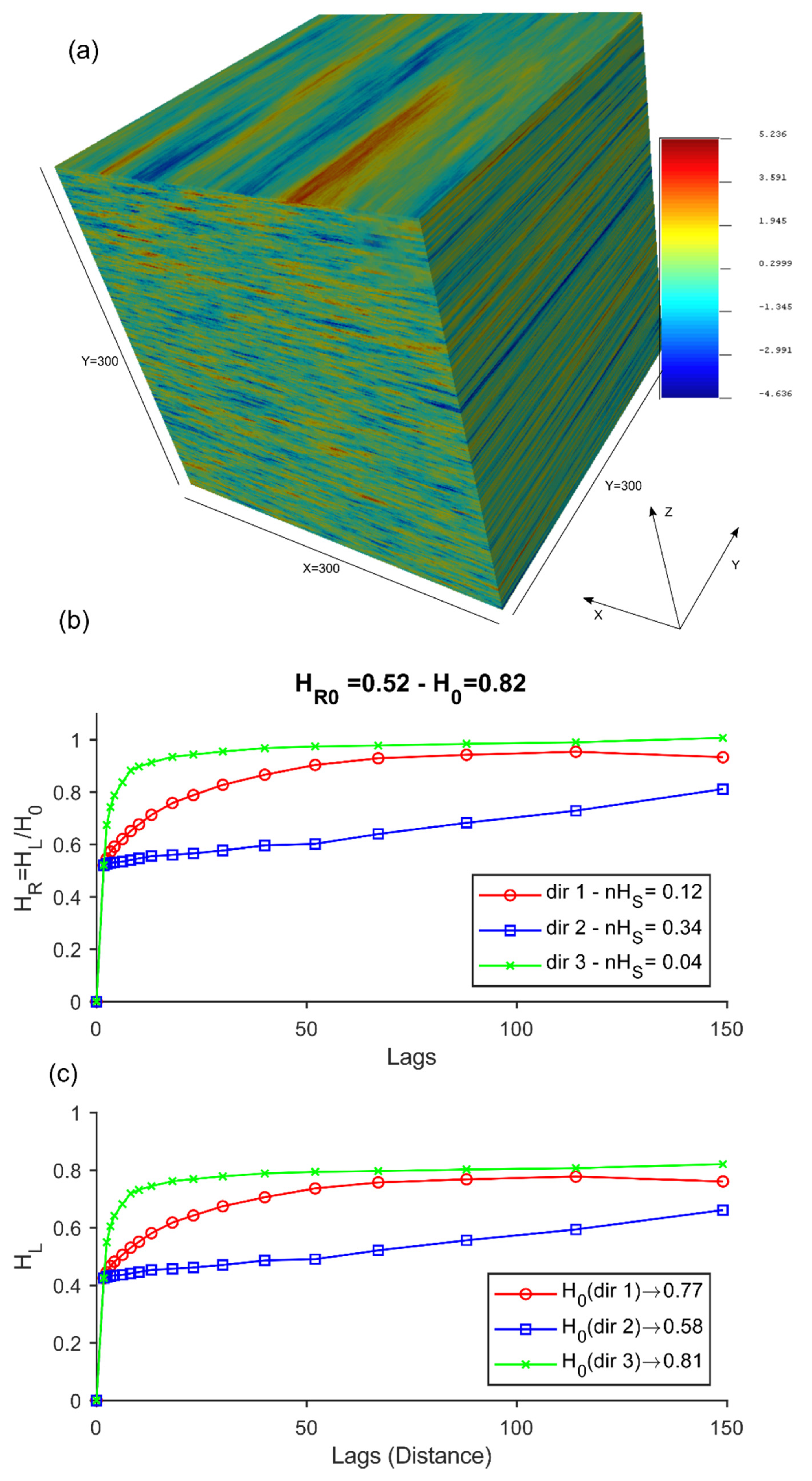
An initial illustrative example of geological entropy analysis with GEOENT is shown in Figure 4. The dataset in this case is a 3D (300 × 300 × 300 voxels) sequential Gaussian simulation (SGS) continuous field generated using SGEMS [26]. The random spatial field was created using a spherical anisotropic variogram with a range of 300 voxels over Y, 30 voxels over X, and 3 voxels over Z. The resulting dataset shows well-defined directional correlations of the simulated generic variable (Figure 4a). The correlation is longer over Y than that over X, which is, in turn, longer than that over Z.
To carry out the analyses, we set the following features:
- In Block 1, NJ = 300; NI = 300; NK = 300; dx = 1; dy = 1; dz = 1 (corresponding to the specific directions of this dataset). Since the dataset was already saved as a GSLIB format, it was directly imported into MATLAB without format transformation;
- In Block 2, Ncat = 5, such that the continuous variable distribution is binned into five categories;
- In Block 3, NMC = 500, such that the number of repetitions to compute the ensemble averages of entrograms in each direction is 500; loglag = true, such that lags are computed logarithmically; lagsteplogspace = 20, which is the number of steps of the logarithmically spaced lags;
- In Block 4, bandwidth_X = 300, bandwidth_Y = 1, and bandwidth_Z = 1, such that the maximum size (number of voxels) of the searching box is 300 × 1 × 1 over X, Y, and Z when the strike and dip angles ‘alpha’ and ‘beta’ are = 0° and = 0°, respectively;
- In Block 45, NUMDIR = 3, such that we compute three directional entrograms, each one defined by the directions specified by ‘alpha’ and ‘beta’ angles. We also set alpha = {0. 90. 0.} and beta = {0. 0. 90.}, such that the first entrogram is oriented over the x direction, the second entrogram is oriented over the y axis, and the third entrogram is oriented over the z direction. We finally set nHs_flag = 1, after which normalised entrograms were plotted.
The three entrograms and corresponding metrics are plotted in Figure 4b. The top panel shows the normalised entrograms, i.e., the change in relative entropy with the lags, for each direction. The title shows the relative entropy of the first lag, and the global entropy, The legend of the top plot reports the entropic scale (here, the normalised entropy scale, ) for each direction. The bottom plot shows the non-normalised entrograms, i.e., the change in local entropy with the lags for each direction. The legend of the bottom plot reports the global entropy for each i-th direction, . This value is computed by averaging H_L over the last three calculated lags, assuming that for a sufficiently wide lag range, .
In the analysed 3D SGS dataset, we found a global entropy = 0.82, which can be considered a large number since the maximum global entropy (i.e., the maximum disorder) is . This means the analysed 3D dataset is fairly disordered when considered as a whole. The relative entropy at lag 1 is = 0.52. The relative information of the spatial order provided by this value depends on the specific application for which geological entropy is used. For instance, for solute transport modelling, Bianchi and Pedretti [14] found that alluvial aquifers characterised by = 0.5 have an intermediate potential of generating preferential flow and solute channelling, eventually leading to non-Fickian transport.
The new functionality introduced by GEOENT is the evaluation of the anisotropic order of the system, which is estimated by the scaling of the directional entrograms. In this application, we found that is larger for dir 2 (oriented along the y axis), with = 0.34, than for dir 1 (oriented over the x axis), with = 0.12, which, in turn, is larger than dir 2 (oriented over the z axis), with = 0.04. These values are consistent with the shape of the entrograms, which show a more rapid increase towards in the z direction than in the y direction, which is, in turn, more rapid than in the x direction. The different scaling of the entrograms and corresponding entropic scales agree with the anisotropic structure of the 3D SGS, which was created using a directional variogram showing a larger correlation range in the y direction than in the x direction, which was, in turn, larger than in the z direction.
A similar conclusion is drawn from the analysis of the global entropy, . In dir 1 (oriented over y), with the system remains globally more ordered than over the other directions, which instead show values that tend towards the global entropy This means that, over x and z axes, the system is as chaotic and disordered as the entire system, when taken as a whole. By contrast, over the y axis, the system would require more space to show the same degree of disorder as the global system.
3.2. Two-Dimensional (2D) Training Images
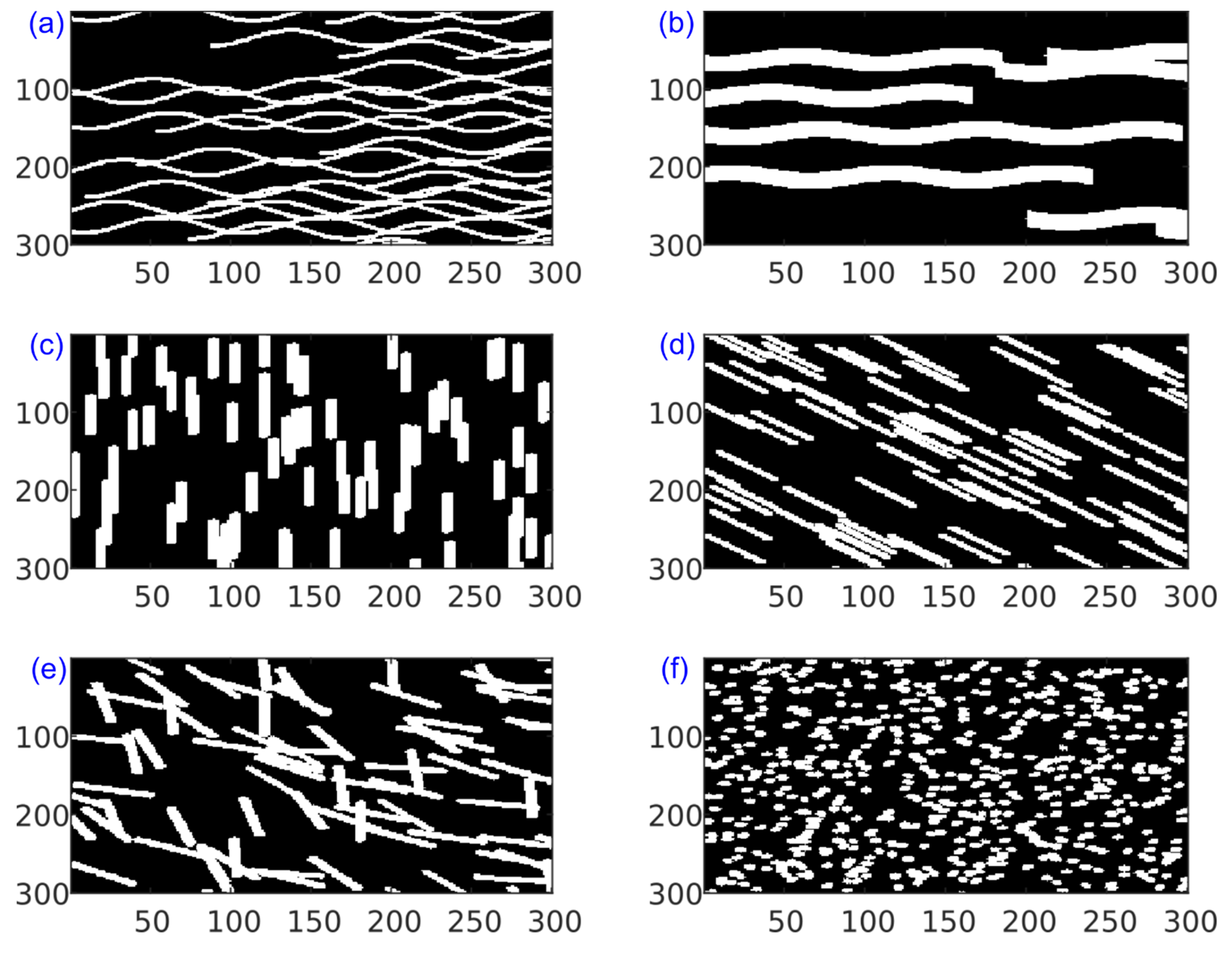
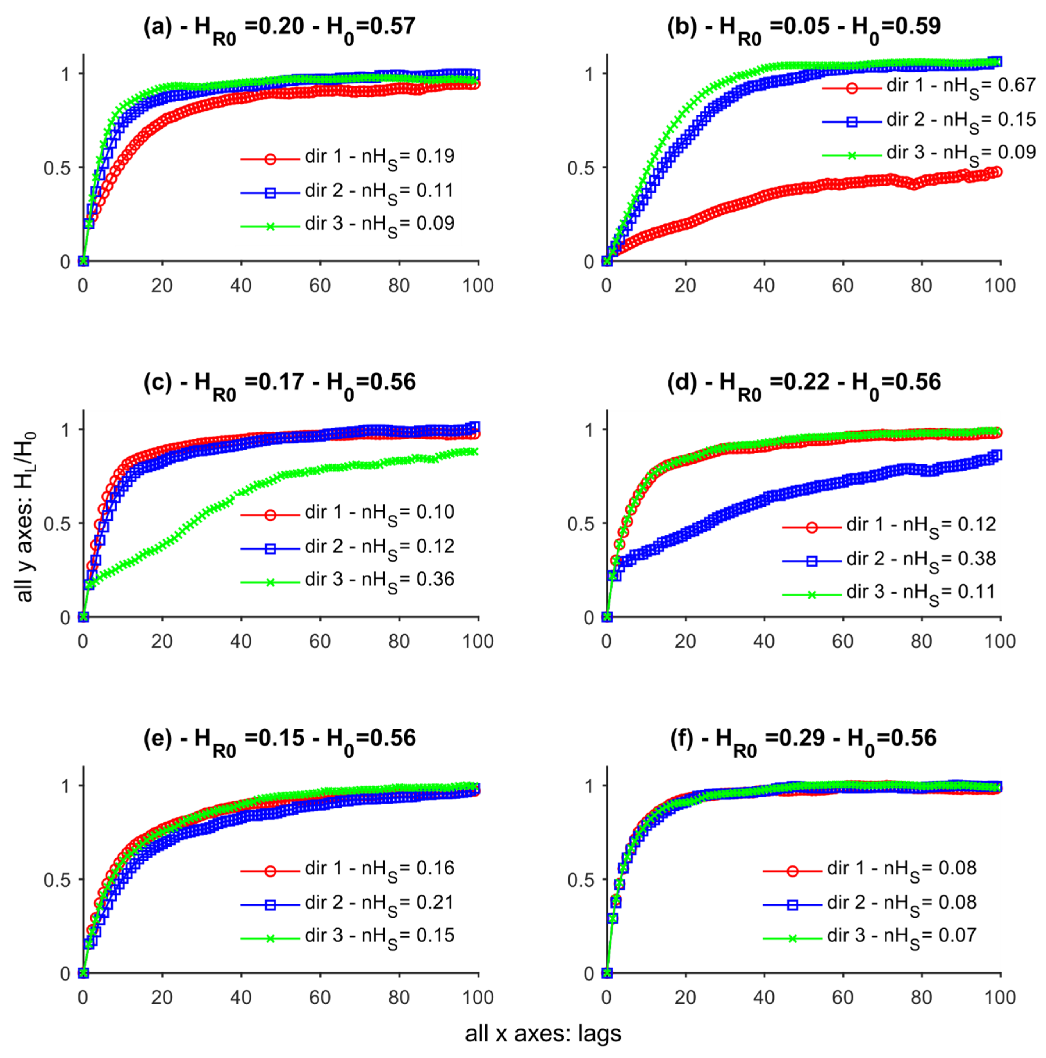
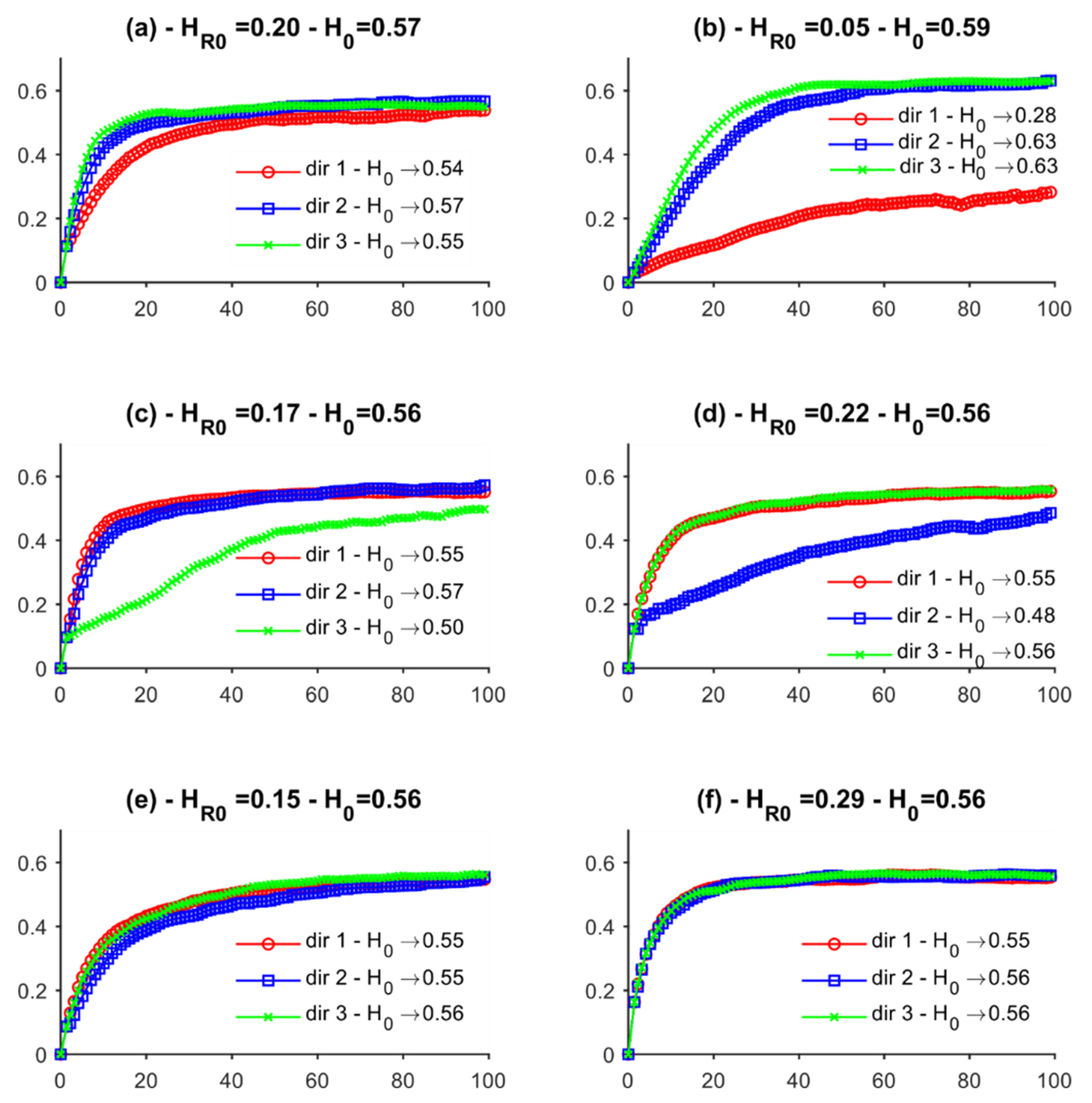
We now show how GEOENT is able to evaluate the spatial order in a series of two-dimensional (2D) training images (TIs). Such images are commonly used in multipoint geostatistical analyses [27,28,29] to generate realistic features in various geological environments. The analysed dataset, shown in Figure 5, consists of six images of 300 × 300 pixels generated using the code TiGenerator [28], an SGEMS plugin that creates TIs with discretised categories (called ‘geobodies’) that resemble geological features, such as alluvial depositional environments. In our analysis, we considered a single geobody embedded into the complementary background matrix, resulting in NCAT = 2. While the shape of the geobody is set to be ‘sinusoid’ in all generated Tis, and the relative proportion is the same (25:75), the geometry of the geobody is different in each TI, owing to the different properties adopted in TiGenerator, as defined in Table 1. The resulting directional entrograms and corresponding metrics are shown in Figure 6 and Figure 7, respectively, for the normalised and non-normalised entrograms. We computed three directions (NDIR=0), with ° for dir 1 (parallel to the horizontal axis (x)), with ° for dir 2, and with ° for dir 3 (parallel to the vertical axis (y)).
For Figure 5a,b, the corresponding entrograms in Figure 6 and Figure 7 show a larger order over the x axis, which agrees well with the visual shape of the geobodies, being longer and more connected over that direction than over the other. This is due to the selected orientation of the geobodies. Despite the same length of the geobodies, the entrograms indicate that the TI (a) is more disordered than TI (b). The normalised entrograms scales () in all directions are smaller in TI (a) than in TI (b), particularly for what concerns dir 1. This is explained considering that, in TI (a), the narrow size of the geobodies determines a larger number of geobodies in the image to reach the desired proportion of facies. In TI (b), by contrast, the thicker shape of the geobodies hides their sinusoidal shape. As such, TI (b) results is a much more regular and stratified image, which is correctly reflected by different values. The other geological entropy metric, , is also lower in TI (b) than in TI (a), agreeing with the previous conclusions by Bianchi and Pedretti [14], which found higher order of random spatial fields when .
For Figure 5c,d, the corresponding entrograms in Figure 6 and Figure 7 correctly reproduce the different orientations of the geobodies. In TI (c), the orientation is mainly vertical, and the entrograms correctly reproduce a higher order for dir 3, which is parallel to the y axis. In TI (d), the orientation is tilted by 45°, and the entrograms corresponding to dir 2 are now suggesting a longer spatial order over that direction.
3.3. Three-Dimensional (3D) X-ray Microtomography Images
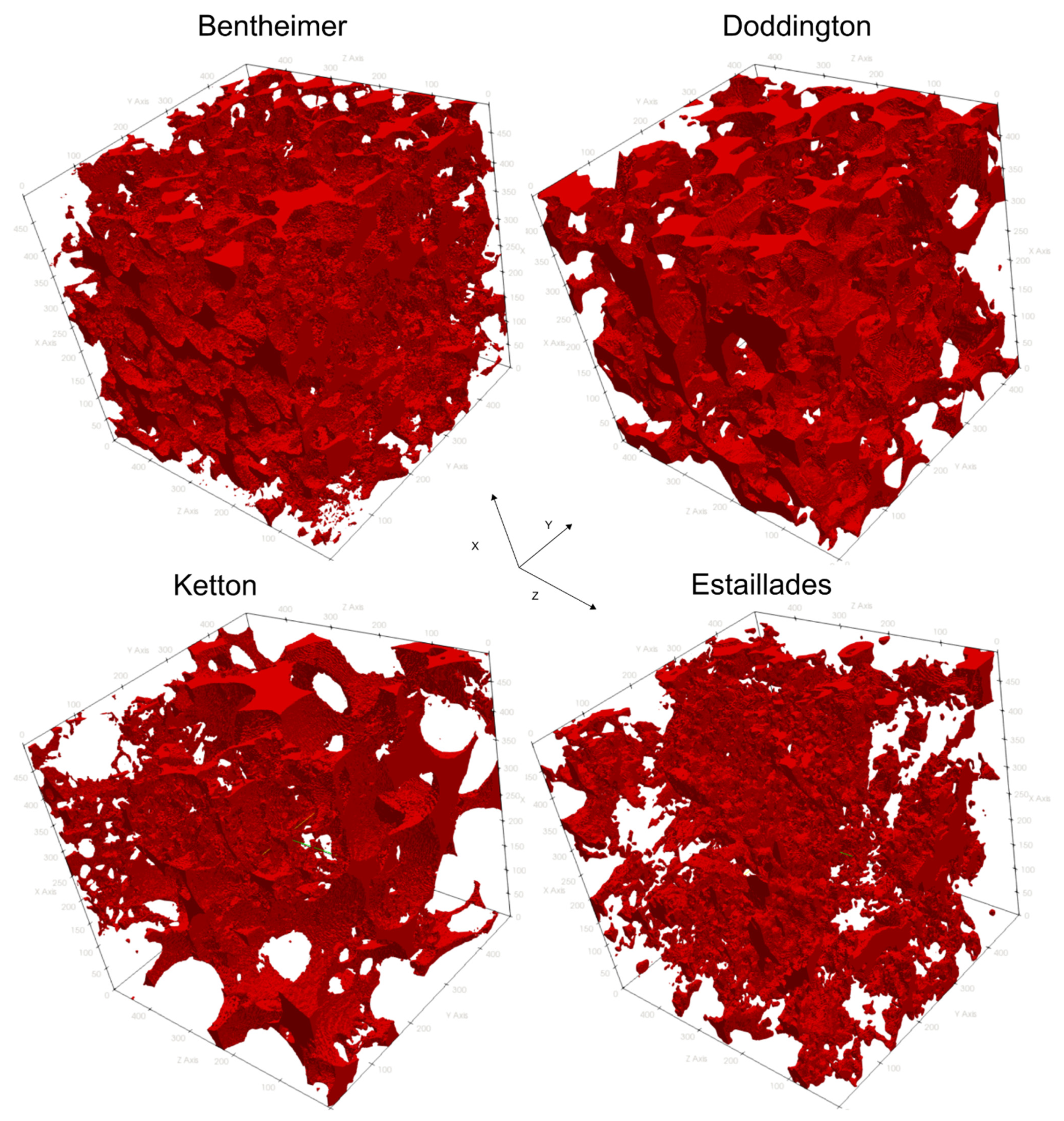
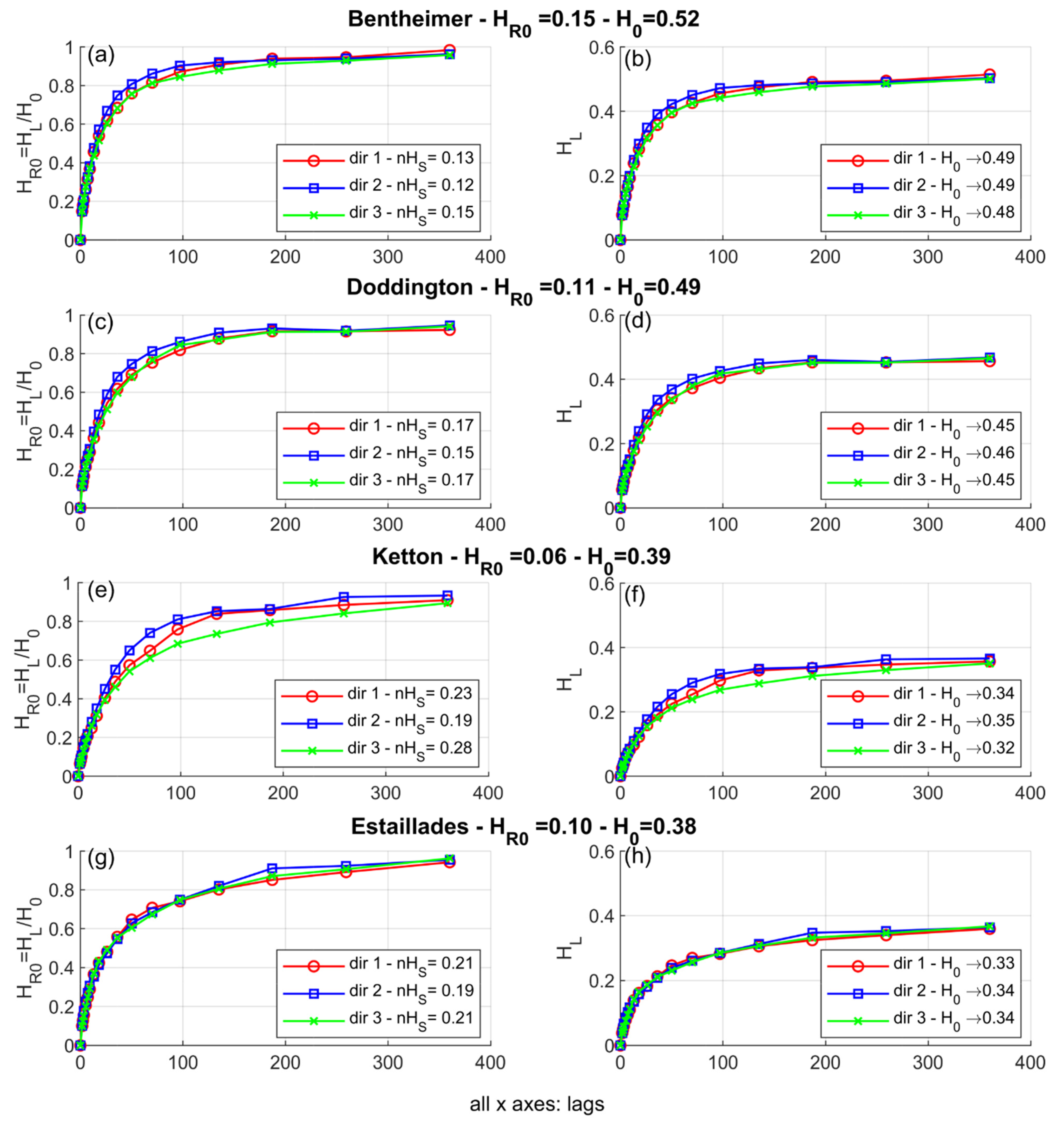
Another example of the application of GEOENT considers three-dimensional (3D) digitalized images obtained from X-ray microtomography (μCT) [30,31,32,33,34,35,36]. GEOENT was used to assess the spatial structure of four well-studied digitalised rock samples, two sandstones (Bentheimer and Doddington), and two carbonates (Estaillades and Ketton). These images have been particularly useful to develop/prove new theories of transport in heterogeneous media, such as the use of upscaling models to predict ‘anomalous’ (i.e., non-Fickian) transport emerging in heterogeneous systems as a consequence of the different textural properties of these rocks [37,38,39,40].
The images were scanned at the Imperial College of London (available at https://www.imperial.ac.uk/earth-science/research/research-groups/pore-scale-modelling/micro-ct-images-and-networks/; accessed on 28 February 2022). Each image has a total of 10003 voxels, providing a useful testing scenario to evaluate the efficiency of GEOENT to process large-scale datasets. The images have voxel resolutions of 3.0035 μm for the Bentheimer sample, 2.6929 μm for the Doddington sample, 3.31136 μm for the Estaillades sample, and 3.00006 μm for the Ketton sample. The images were segmented to represent a binary distribution, where ‘0’ corresponds to the solid matrix, and ‘1’ to the void space. The chosen images (Figure 8) show different textural arrangements, resulting in different grain-size distributions and spatial organization of the pore space. The samples are described in detail in Andrew et al. [38].
The entrograms calculated with GEOENT (Figure 9) indicate shorter entropic scales for the sandstones compared with the carbonates, and therefore, the sandstones have higher degrees of spatial disorder in the solid/void distribution. This agrees well with the more homogeneous pore- and grain-size distribution in the sandstones, as visually appreciated from a close inspection of Figure 8. The global entropy is also larger in the sandstones than in the carbonates, indicating that globally, the carbonates show higher spatial order than the sandstones, which are instead more mixed and chaotic. The relative entropy at the first lag () is lower in carbonates than in the sandstone. Recalling the analysis by Bianchi and Pedretti [14]), this suggests that the nature of solute transport in carbonates s to be more non-Fickian than in sandstones, which is consistent with the general understanding of transport in these types of rocks [20].
Comparing Ketton and Estaillades entrograms, we found that both digitalised rock samples are characterised by a very similar global entropy ( = 0.39 for Ketton and = 0.38 for Estaillades). The relative entropy at the first lag is also similar but slightly lower in Ketton ( = 0.06) than in Estaillades ( = 0.1). Both values are low, further confirming that, at the scale of the image resolution (3 μm), the probability that both rock samples generate preferential flow is high. Indeed, < 0.1 was found to generate BTC skewness in the simulations by Bianchi and Pedretti [14] for different values of the variance of the log-transformed hydraulic conductivity of the flow field. However, the lower in Ketton than in Estaillades means that Ketton may have a slightly higher probability to generate non-Fickian transport than Estaillades.
We also found that Ketton is more anisotropic than Estaillades. In Ketton, the spatial order is more persistent along the vertical direction (dir 3, = 0.28) than in the plane (dir 1, = 0.23; dir 2, = 0.19). The anisotropic entrogram describing the spatial order of the Ketton sample is consistent with the analysis by Mosser et al. (2017), who reported the anisotropic behaviour of the covariance used to describe the spatial structure of the same sample. In Estaillades, the spatial order is instead more comparable among the different directions but always lower than dir 1 in Ketton. This is a further confirmation that Ketton could produce more non-Fickian transport than Estaillades.
3.4. Three-Dimensional (3D) Aquifer Analogues
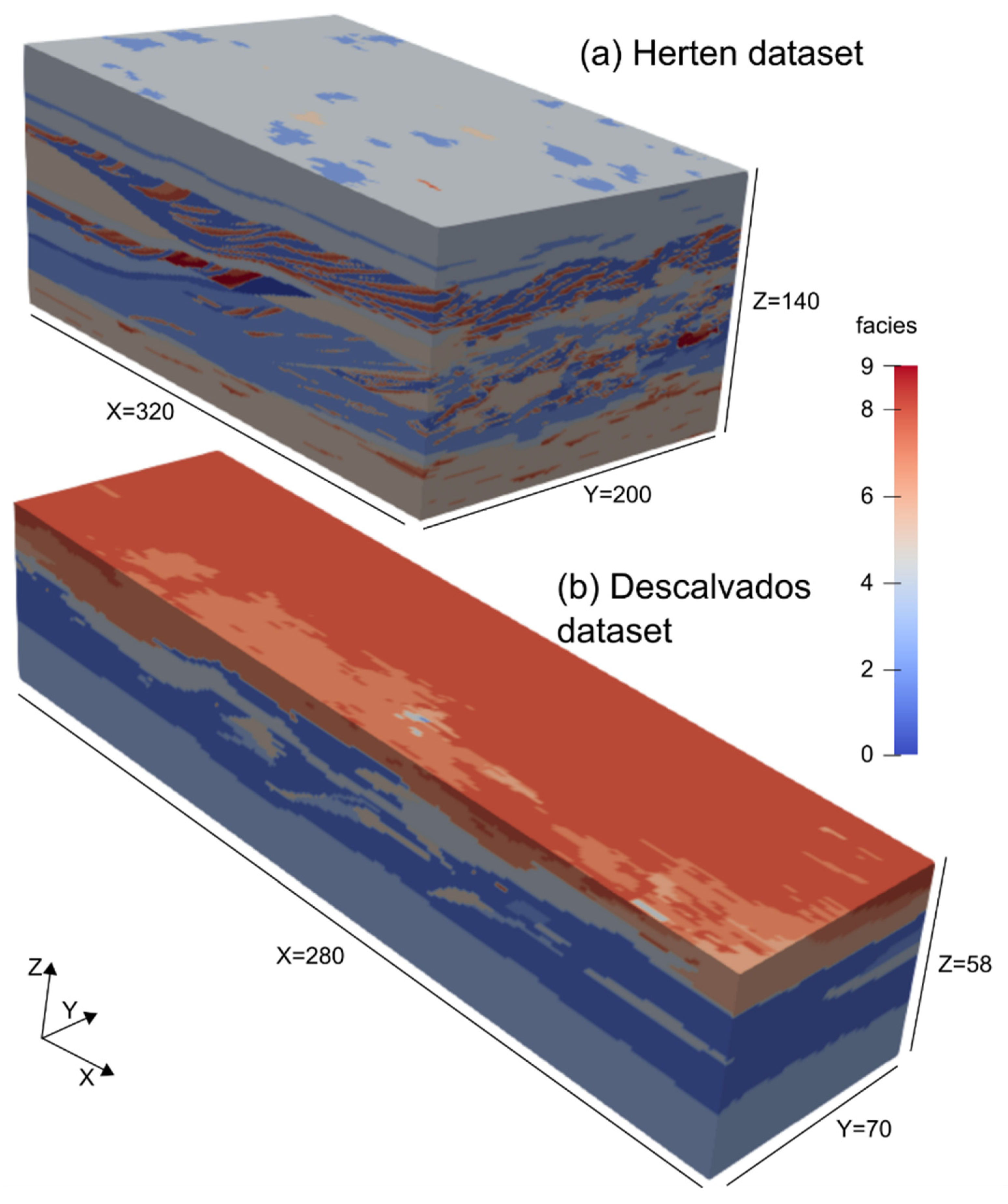
The last example of the application of GEOENT focuses on the evaluation of 3D aquifer analogues. These are detailed field descriptions of the heterogeneity of outcropping sedimentary deposits that can be used to study fluid flow in the subsurface [27,41,42] or the architectural geometries of petroleum reservoirs [43]. Such analogues are based on direct observations of the lithology and sedimentary structure and geophysical surveys. The specific datasets evaluated in this study reproduce two well-known aquifer analogues [41]:
- The Descalvado aquifer, described as a moderately heterogeneous fluvial–aeolian deposit of the upper part of the Pirambóia Formation (Triassic) of south-eastern Brazil [44].
Bayer et al. [41] provided a comprehensive set of realizations based on multipoint geostatistics that stochastically reproduce the variation of categorised facies in each analogue. Two of these realizations are presented in Figure 10. In (a), the Herten dataset is shown. The volume is composed of 320 × 200 × 140 unit-size voxels. From a visual assessment, the Herten dataset shows a well-defined variation of the facies’ proportions over the vertical direction (z) and a stratified structure l. The Descalvado dataset, shown in (b), is composed of 280 × 140 × 70 unit-size voxels. From a visual assessment, the Descalvado aquifer analogue also shows a well-defined stratification, with a shorter correlation of the facies over the z direction than over the x and y directions. Visually, it is difficult to assess the presence of anisotropic structures in both samples.
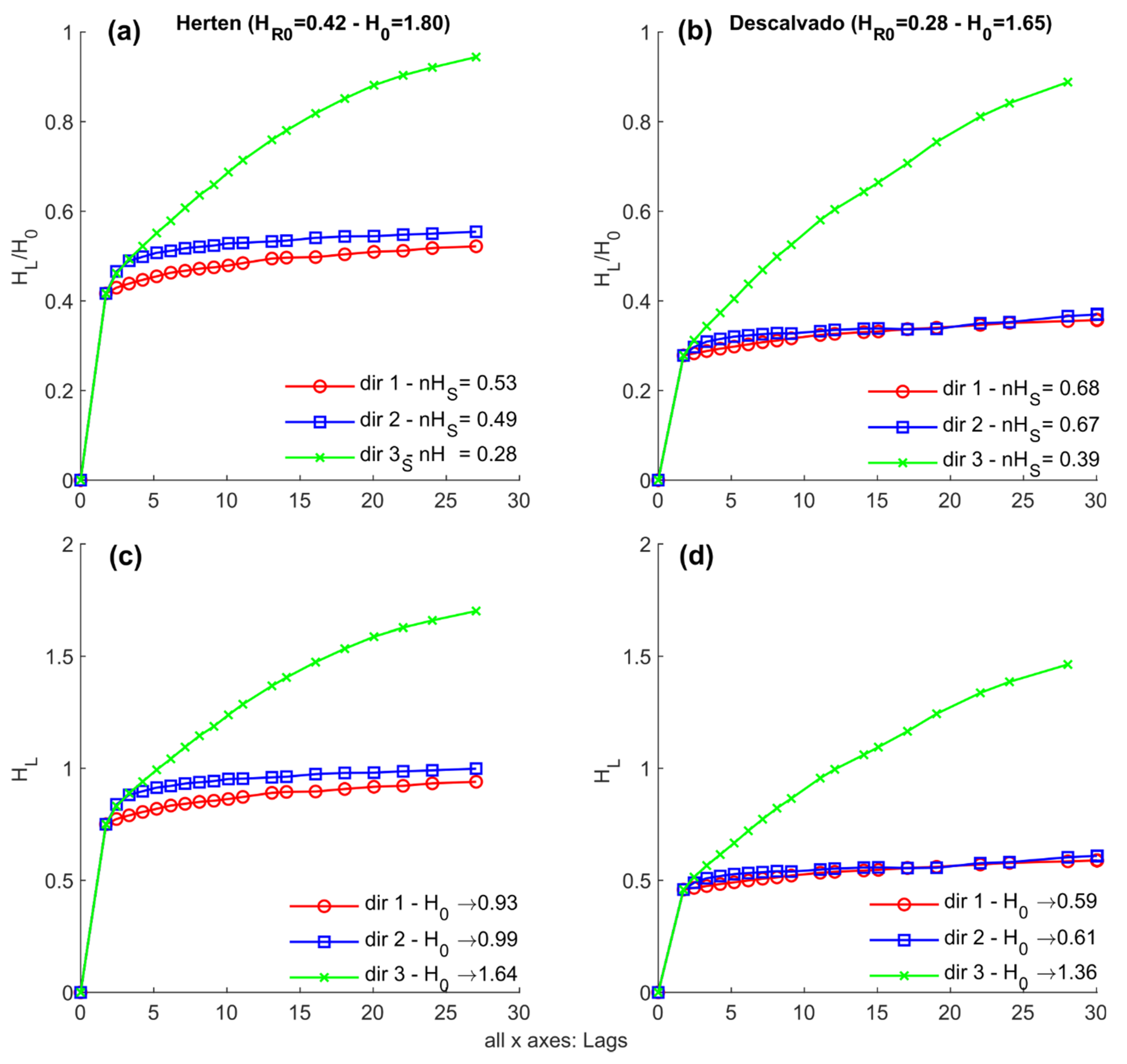
The directional entrograms of both analogues are compared in Figure 11. At the top, the panels (a) and (b) show the normalised entrograms. We found that the spatial order is much more continuous along the horizontal planes than over the vertical direction, consistent with the visual assessment of the analogue’s volumes shown in Figure 10. The normalised entropic scale, , is shorter over z in both samples. The comparison between the two datasets revealed however that the spatial order is more persistent in the Descalvado analogue than in the Herten analogue. At Descalvado, the entrograms along x and y are flatter than in Herten, as quantified by the lower in Descalvado (dir 1, = 0.68; dir 2, = 0.67) than in Herten (dir 1, = 0.53; dir 1, = 0.49). The analysis revealed that, in the plane, Herten is also more anisotropic than Descalvado. This conceptually agrees with the genetic origin of Herten (fluvioglacial, braided river sediment), which tends to generate alluvial deposits preferentially oriented over one direction. The fluvial–aeolian nature of the Descalvado deposits is instead more prone to generating more isotropic deposits.
The relative geological entropy at the first lag, , is lower in Descalvado than in Herten. At the bottom, the panels (c) and (d) show the non-normalized entrograms, which suggest that the global entropy is lower for the Descalvado analogue than for the Herten analogue. The directional global entropies in the plane ( are also generally lower in Descalvado.
To extrapolate these results in the context of predicting transport behaviour in the two aquifers, it is important to note that our focus here is only on the lithological composition and not on the distribution of hydraulic conductivity. In fact, Bianchi and Pedretti [14] showed that the tendency of a system to generate non-Fickian transport is linked to as well as the variance in the log-transformed hydraulic conductivity (), which is much larger in Herten ( = 5.13) than in Descalvado ( = 1.91) [45]. More proper and rigorous solute transport analyses will be presented in the future to evaluate each individual case study and draw more pertinent case-specific conclusions.
4. Conclusions
The analysis of gridded datasets representing the spatial distribution of categorical or continuous variables is essential in a wide range of disciplines. In geological sciences, readily available software packages that can be applied to analyse the spatial variability of heterogeneous systems are usually based on variogram-based geostatistical approaches [25]. GEOENT differs from these by describing spatial variability with an information entropy-based approach, which quantifies the degree of spatial association and order of the considered field.
An important novelty of GEOENT is that it incorporates an updated algorithm for calculating the entrogram, which allows the detection of anisotropy in spatial structures and, therefore, allows one to evaluate the degrees of spatial order in different directions. Anisotropy is commonly observed in the spatial arrangement of heterogeneous categorical and continuous data. Without such capability, some salient directional differences in the analysed datasets would not be appreciated, as we showed here using examples ranging from relatively simple 2D binary images to complex reconstructions of lithological variability in sedimentary aquifers. The geological entropy metrics calculated with GEOENT have the potential to provide insight to explain complex physical processes occurring in heterogeneous systems, such as fluid flow or solute transport [14,15] The development of robust theories for different fields is the topic of ongoing and future research.
Author Contributions
Conceptualisation, methodology, software development, data curation, writing—original draft preparation, D.P. and M.B. All authors have read and agreed to the published version of the manuscript.
Funding
This research received no external funding.
Institutional Review Board Statement
Not applicable.
Informed Consent Statement
Not applicable.
Data Availability Statement
GEOENT is available in a GitHub repository (https://github.com/hydrogeolab/GEOENT) (accessed on 3 January 2022), in which it is distributed under GNU Lesser General Public License v3.0.
Acknowledgments
The results here presented were developed in the frame of the MIUR Project ‘Dipartimenti di Eccellenza 2017—Le Geoscienze per la società: risorse e loro evoluzione’.
Conflicts of Interest
The authors declare no conflict of interest.
Appendix A. Shannon Information Entropy
The Shannon information entropy () [1] lies at the core of the geological entropy approach. This entropy quantifies the amount of information contained in a random source of information. Mathematically, is defined analogously to the Boltzmann–Gibbs thermodynamic entropy. In statistical mechanics, entropy is interpreted as a measure of the disorder of a physical system. The frame of geological entropy provides a measure of the disorder of a geological system.
For an event released by a generic source , also known as self-information, the information () is calculated as
where is the probability of occurrence of that event. The logarithm stems from the need to compute the total entropy of an independent event, for which the probability is the product of the individual probabilities. The information entropy is defined as the expected or mean data contained in a single message and are computed as
For a discrete random variable containing events, is calculated as the mean data of the individual event , which is
References
- Shannon, C.E. A Mathematical Theory of Communication. Bell Syst. Tech. J. 1948, 27, 379–423. [Google Scholar] [CrossRef] [Green Version]
- Schug, J.; Schuller, W.-P.; Kappen, C.; Salbaum, J.M.; Bucan, M.; Stoeckert, C.J. Promoter Features Related to Tissue Specificity as Measured by Shannon Entropy. Genome Biol. 2005, 6, R33. [Google Scholar] [CrossRef] [PubMed] [Green Version]
- Kress, G.; Van Leeuwen, T. Reading Images: The Grammar of Visual Design; Routledge: London, UK, 2020. [Google Scholar]
- Zhou, R.; Cai, R.; Tong, G. Applications of Entropy in Finance: A Review. Entropy 2013, 15, 4909–4931. [Google Scholar] [CrossRef]
- Zhu, S.; Zhu, C.; Wang, W. A New Image Encryption Algorithm Based on Chaos and Secure Hash SHA-256. Entropy 2018, 20, 716. [Google Scholar] [CrossRef] [PubMed] [Green Version]
- Journel, A.G.; Deutsch, C.V. Entropy and Spatial Disorder. Math. Geol. 1993, 25, 329–355. [Google Scholar] [CrossRef]
- Christakos, G. A Bayesian/Maximum-Entropy View to the Spatial Estimation Problem. Math. Geol. 1990, 22, 763–777. [Google Scholar] [CrossRef]
- Naimi, B.; Hamm, N.A.S.; Groen, T.A.; Skidmore, A.K.; Toxopeus, A.G.; Alibakhshi, S. ELSA: Entropy-Based Local Indicator of Spatial Association. Spat. Stat. 2019, 29, 66–88. [Google Scholar] [CrossRef]
- Pham, T.D. GeoEntropy: A Measure of Complexity and Similarity. Pattern Recognit. 2010, 43, 887–896. [Google Scholar] [CrossRef]
- Thiesen, S.; Vieira, D.M.; Mälicke, M.; Loritz, R.; Wellmann, J.F.; Ehret, U. Histogram via Entropy Reduction (HER): An Information-Theoretic Alternative for Geostatistics. Hydrol. Earth Syst. Sci. 2020, 24, 4523–4540. [Google Scholar] [CrossRef]
- Wu, Y.; Zhou, Y.; Saveriades, G.; Agaian, S.; Noonan, J.P.; Natarajan, P. Local Shannon Entropy Measure with Statistical Tests for Image Randomness. Inf. Sci. 2013, 222, 323–342. [Google Scholar] [CrossRef] [Green Version]
- Batty, M.; Morphet, R.; Masucci, P.; Stanilov, K. Entropy, Complexity, and Spatial Information. J. Geogr. Syst. 2014, 16, 363–385. [Google Scholar] [CrossRef] [PubMed] [Green Version]
- Wellmann, J.F.; Regenauer-Lieb, K. Uncertainties Have a Meaning: Information Entropy as a Quality Measure for 3-D Geological Models. Tectonophysics 2012, 526–529, 207–216. [Google Scholar] [CrossRef]
- Bianchi, M.; Pedretti, D. Geological Entropy and Solute Transport in Heterogeneous Porous Media. Water Resour. Res. 2017, 53, 4691–4708. [Google Scholar] [CrossRef] [Green Version]
- Bianchi, M.; Pedretti, D. An Entrogram-Based Approach to Describe Spatial Heterogeneity with Applications to Solute Transport in Porous Media. Water Resour. Res. 2018, 54, 4432–4448. [Google Scholar] [CrossRef]
- Pedretti, D. Heterogeneity-Controlled Uncertain Optimization of Pump-and-Treat Systems Explained through Geological Entropy. Int. J. Geomath. 2020, 11, 22. [Google Scholar] [CrossRef]
- Pedretti, D.; Bianchi, M. Preliminary Results from the Use of Entrograms to Describe Transport in Fractured Media. Acque Sotter. Ital. J. Groundw. 2019, 8. [Google Scholar] [CrossRef]
- Ye, Z.; Jiang, Q.; Yao, C.; Liu, Y.; Cheng, A.; Huang, S.; Liu, Y. The Parabolic Variational Inequalities for Variably Saturated Water Flow in Heterogeneous Fracture Networks. Geofluids 2018, 2018, 9062569. [Google Scholar] [CrossRef] [Green Version]
- Ye, Z.; Fan, X.; Zhang, J.; Sheng, J.; Chen, Y.; Fan, Q.; Qin, H. Evaluation of Connectivity Characteristics on the Permeability of Two-Dimensional Fracture Networks Using Geological Entropy. Water Resour. Res. 2021, 57, e2020WR029289. [Google Scholar] [CrossRef]
- Bijeljic, B.; Mostaghimi, P.; Blunt, M.J. Insights into Non-Fickian Solute Transport in Carbonates: Insights into Non-Fickian Solute Transport in Carbonates. Water Resour. Res. 2013, 49, 2714–2728. [Google Scholar] [CrossRef] [Green Version]
- Berkowitz, B.; Scher, H. On Characterization of Anomalous Dispersion in Porous and Fractured Media. Water Resour. Res. 1995, 31, 1461–1466. [Google Scholar] [CrossRef]
- Hyman, J.D.; Aldrich, G.; Viswanathan, H.; Makedonska, N.; Karra, S. Fracture Size and Transmissivity Correlations: Implications for Transport Simulations in Sparse Three-Dimensional Discrete Fracture Networks Following a Truncated Power Law Distribution of Fracture Size. Water Resour. Res. 2016, 52, 6472–6489. [Google Scholar] [CrossRef]
- Koltermann, C.E.; Gorelick, S. Heterogeneity in Sedimentary Deposits: A Review of Structure-Imitating, Process-Imitating, and Descriptive Approaches. Water Resour. Res. 1996, 32, 2617–2658. [Google Scholar] [CrossRef]
- Scheibe, T.D. Characterization of the Spatial Structuring of Natural Porous Media and Its Impacts on Subsurface Flow and Transport. Ph.D. Thesis, Stanford University, Stanford, CA, USA, 1993. [Google Scholar]
- Deutsch, C.V.; Journel, A.G. GSLIB: Geostatistical Software Library and User’s Guide; Oxford University Press: Oxford, UK, 1998; ISBN 978-0-19-510015-0. [Google Scholar]
- Remy, N.; Boucher, A.; Wu, J. Applied Geostatistics with SGeMS. A User’s Guide; Cambridge University Press: New York, NY, USA, 2009. [Google Scholar]
- Comunian, A.; Renard, P.; Straubhaar, J.; Bayer, P. Three-Dimensional High Resolution Fluvio-Glacial Aquifer Analog—Part 2: Geostatistical Modeling. J. Hydrol. 2011, 405, 10–23. [Google Scholar] [CrossRef] [Green Version]
- Maharaja, A. TiGenerator: Object-Based Training Image Generator. Comput. Geosci. 2008, 34, 1753–1761. [Google Scholar] [CrossRef]
- Strebelle, S. Conditional Simulation of Complex Geological Structures Using Multiple-Point Statistics. Math. Geol. 2002, 34, 1–21. [Google Scholar] [CrossRef]
- Flannery, B.P.; Deckman, H.W.; Roberge, W.G.; D’Amico, K.L. Three-Dimensional X-Ray Microtomography. Science 1987, 237, 1439–1444. [Google Scholar] [CrossRef]
- Blunt, M.J.; Bijeljic, B.; Dong, H.; Gharbi, O.; Iglauer, S.; Mostaghimi, P.; Paluszny, A.; Pentland, C. Pore-Scale Imaging and Modelling. Adv. Water Resour. 2013, 51, 197–216. [Google Scholar] [CrossRef] [Green Version]
- Le Gros, M.A.; McDermott, G.; Larabell, C.A. X-Ray Tomography of Whole Cells. Curr. Opin. Struct. Biol. 2005, 15, 593–600. [Google Scholar] [CrossRef]
- Otten, W.; Pajor, R.; Schmidt, S.; Baveye, P.C.; Hague, R.; Falconer, R.E. Combining X-Ray CT and 3D Printing Technology to Produce Microcosms with Replicable, Complex Pore Geometries. Soil Biol. Biochem. 2012, 51, 53–55. [Google Scholar] [CrossRef] [Green Version]
- Reijonen, H.M. Benefits of Applying X-Ray Computed Tomography in Bentonite Based Material Research Focussed on Geological Disposal of Radioactive Waste. Env. Sci. Pollut. Res. 2020, 15, 38407–38421. [Google Scholar] [CrossRef] [Green Version]
- Sayab, M.; Suuronen, J.-P.; Hölttä, P.; Aerden, D.; Lahtinen, R.; Kallonen, A.P. High-Resolution X-Ray Computed Microtomography: A Holistic Approach to Metamorphic Fabric Analyses. Geology 2015, 43, 55–58. [Google Scholar] [CrossRef]
- Yang, Y.; Tao, L.; Iglauer, S.; Hejazi, S.H.; Yao, J.; Zhang, W.; Zhang, K. Quantitative Statistical Evaluation of Micro Residual Oil after Polymer Flooding Based on X-Ray Micro Computed-Tomography Scanning. Energy Fuels 2020, 34, 10762–10772. [Google Scholar] [CrossRef]
- Alhashmi, Z.; Blunt, M.J.; Bijeljic, B. The Impact of Pore Structure Heterogeneity, Transport, and Reaction Conditions on Fluid–Fluid Reaction Rate Studied on Images of Pore Space. Transp. Porous. Med. 2016, 115, 215–237. [Google Scholar] [CrossRef] [Green Version]
- Andrew, M.; Bijeljic, B.; Blunt, M.J. Pore-Scale Imaging of Trapped Supercritical Carbon Dioxide in Sandstones and Carbonates. Int. J. Greenh. Gas Control 2014, 22, 1–14. [Google Scholar] [CrossRef] [Green Version]
- Honari, A.; Bijeljic, B.; Johns, M.L.; May, E.F. Enhanced Gas Recovery with CO2 Sequestration: The Effect of Medium Heterogeneity on the Dispersion of Supercritical CO2–CH4. Int. J. Greenh. Gas Control 2015, 39, 39–50. [Google Scholar] [CrossRef] [Green Version]
- Mosser, L.; Dubrule, O.; Blunt, M.J. Reconstruction of Three-Dimensional Porous Media Using Generative Adversarial Neural Networks. Phys. Rev. E 2017, 96, 043309. [Google Scholar] [CrossRef] [Green Version]
- Bayer, P.; Comunian, A.; Höyng, D.; Mariethoz, G. High Resolution Multi-Facies Realizations of Sedimentary Reservoir and Aquifer Analogs. Sci. Data 2015, 2, 150033. [Google Scholar] [CrossRef] [Green Version]
- Bayer, P.; Huggenberger, P.; Renard, P.; Comunian, A. Three-Dimensional High Resolution Fluvio-Glacial Aquifer Analog: Part 1: Field Study. J. Hydrol. 2011, 405, 1–9. [Google Scholar] [CrossRef] [Green Version]
- Pringle, J.K.; Westerman, A.R.; Clark, J.D.; Drinkwater, N.J.; Gardiner, A.R. 3D High-Resolution Digital Models of Outcrop Analogue Study Sites to Constrain Reservoir Model Uncertainty: An Example from Alport Castles, Derbyshire, UK. Pet. Geosci. 2004, 10, 343–352. [Google Scholar] [CrossRef]
- Höyng, D.; D’Affonseca, F.M.; Bayer, P.; de Oliveira, E.G.; Perinotto, J.A.J.; Reis, F.; Weiß, H.; Grathwohl, P. High-Resolution Aquifer Analog of Fluvial–Aeolian Sediments of the Guarani Aquifer System. Env. Earth Sci. 2014, 71, 3081–3094. [Google Scholar] [CrossRef]
- Höyng, D.; Prommer, H.; Blum, P.; Grathwohl, P.; Mazo D’Affonseca, F. Evolution of Carbon Isotope Signatures during Reactive Transport of Hydrocarbons in Heterogeneous Aquifers. J. Contam. Hydrol. 2015, 174, 10–27. [Google Scholar] [CrossRef] [PubMed]
Figure 1.
Conceptual example of the algorithm used by GEOENT to compute the directional entrograms: (a) searching boxes are parallel to the horizontal axis (direction 1, °); (b) searching boxes are parallel to the vertical axis (direction 2, °); (c) normalised directional entrograms; (d) non-normalised directional entrograms.

Figure 2.
Angles and size (‘bandwidth’) that define the directional shape of the searching box used to compute local geological entropy.
Figure 2.
Angles and size (‘bandwidth’) that define the directional shape of the searching box used to compute local geological entropy.

Figure 3.
Snapshot of the main script of GEOENT, highlighting Blocks 1 to 5, in which the user introduces the input parameters to perform the calculation.
Figure 3.
Snapshot of the main script of GEOENT, highlighting Blocks 1 to 5, in which the user introduces the input parameters to perform the calculation.

Figure 4.
(a) A 3D (300 × 300 × 300 voxels) anisotropic sequential Gaussian simulation generated using SGEMS; (b,c) entrograms with normalised and non-normalised directions, respectively, of the 3D dataset, computed using GEOENT. The size of the searching box (defined by the ‘bandwidths’) is 300 × 1 × 1. For dir 1, ° and °, such that the searching box is parallel to x. For dir 2, ° and °, such that the searching box is parallel to y. For dir 3, ° and °, such that the searching box is parallel to z.

Figure 5.
Training images generated using the code TiGenerator [28], with different spatial orders, orientations, and degrees of connectivity of the different (white) features embedded into a (black) matrix. The parameters used to create the subfigures (a–f) are indicated in Table 1.

Figure 6.
Normalised entrograms of the six analysed training images presented in Figure 5.
Figure 6.
Normalised entrograms of the six analysed training images presented in Figure 5.

Figure 7.
Non-normalised entrograms of the six analysed training images presented in Figure 5.
Figure 7.
Non-normalised entrograms of the six analysed training images presented in Figure 5.

Figure 8.
The four analysed digitalised rock samples downloaded from https://www.imperial.ac.uk/earth-science/research/research-groups/pore-scale-modelling/micro-ct-images-and-networks/ (accessed on 27 July 2021). The images represent a 500 × 500 × 500 subset, processed using a threshold filter. Red colour represents the solid matrix.

Figure 9.
Entrograms and corresponding statistics calculated using GEOENT for each of the four analysed digitalised rock samples. (a,b) Normalized and not-normalized entrograms of the Bentheimer rock samples, respectively; (c,d) Normalized and not-normalized entrograms of the Doddington rock samples, respectively; (e,f) Normalized and not-normalized entrograms of the Ketton rock samples, respectively; (g,h) Normalized and not-normalized entrograms of the Estaillades rock samples, respectively.

Figure 10.
(a) The Herten and (b) Descalvado aquifer analogues analysed in this study.

Figure 11.
Entrograms and corresponding statistics calculated using GEOENT for each of the four analysed analogues. (a) Normalized entrograms for the Herten analogue; (b) normalized entrograms for the Descalvado analogue; (c) Not-normalized entrograms for the Herten analogue; (d) Not-normalized entrograms for the Descalvado analogue.


Table 1.
Parameters set in TiGenerator [28] to create the TIs used in the example. For constant properties, the table shows the ‘Mean’ parameter. For random properties with triangular distribution, the table shows the ‘Mean ({min;max})’ parameter.
Table 1.
Parameters set in TiGenerator [28] to create the TIs used in the example. For constant properties, the table shows the ‘Mean’ parameter. For random properties with triangular distribution, the table shows the ‘Mean ({min;max})’ parameter.
| Image | Length | Width | Orientation | Amplitude | Wavelength |
|---|---|---|---|---|---|
| (a) | 300 | 5 | 90 | 5 | 100 |
| (b) | 300 | 20 | 90 | 5 | 100 |
| (c) | 50 | 5 | 0 | 1 | 1 |
| (d) | 50 | 5 | 135 | 1 | 1 |
| (e) | 50 | 5 | 135 {90;180} | 1 | 100 |
| (f) | 5 | 5 | 90 {45;135} | 1 | 1 |
Publisher’s Note: MDPI stays neutral with regard to jurisdictional claims in published maps and institutional affiliations. |
© 2022 by the authors. Licensee MDPI, Basel, Switzerland. This article is an open access article distributed under the terms and conditions of the Creative Commons Attribution (CC BY) license (https://creativecommons.org/licenses/by/4.0/).
Share and Cite
MDPI and ACS Style
Pedretti, D.; Bianchi, M. GEOENT: A Toolbox for Calculating Directional Geological Entropy. Geosciences 2022, 12, 206. https://0-doi-org.brum.beds.ac.uk/10.3390/geosciences12050206
AMA Style
Pedretti D, Bianchi M. GEOENT: A Toolbox for Calculating Directional Geological Entropy. Geosciences. 2022; 12(5):206. https://0-doi-org.brum.beds.ac.uk/10.3390/geosciences12050206
Chicago/Turabian StylePedretti, Daniele, and Marco Bianchi. 2022. "GEOENT: A Toolbox for Calculating Directional Geological Entropy" Geosciences 12, no. 5: 206. https://0-doi-org.brum.beds.ac.uk/10.3390/geosciences12050206
Note that from the first issue of 2016, this journal uses article numbers instead of page numbers. See further details here.