
Fluvial Transport Model from Spatial Distribution Analysis of Libyan Desert Glass Mass on the Great Sand Sea (Southwest Egypt): Clues to Primary Glass Distribution

 ,
,
Abstract
:
1. Introduction
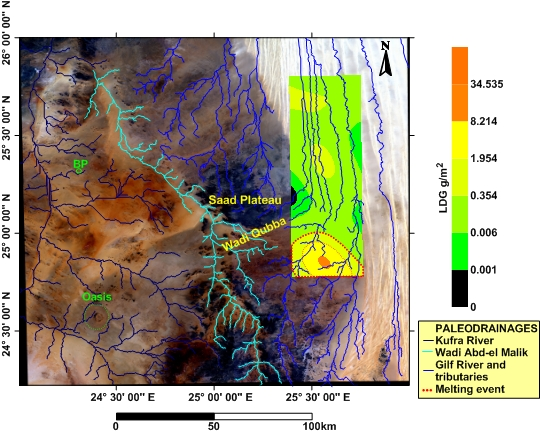
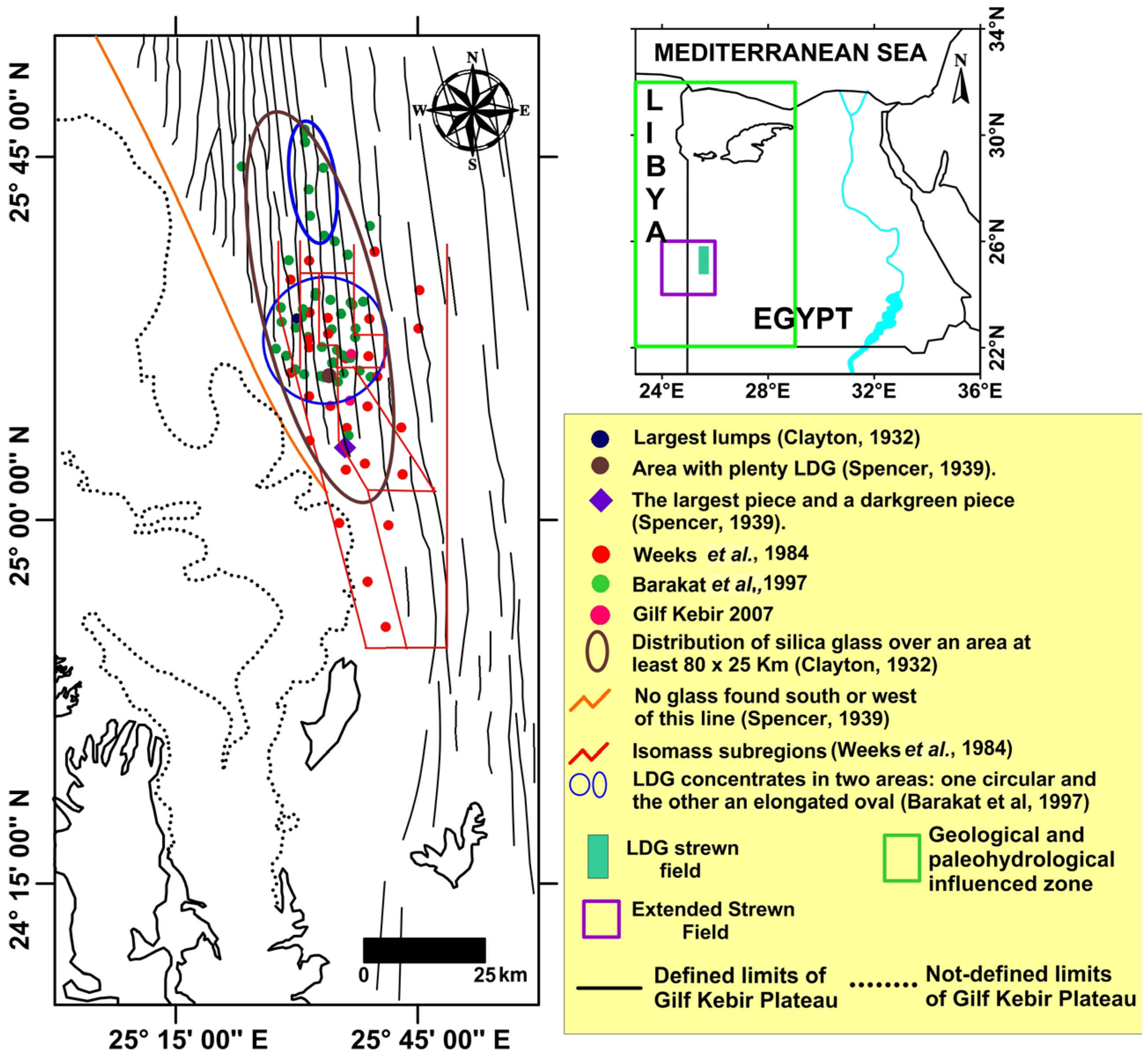
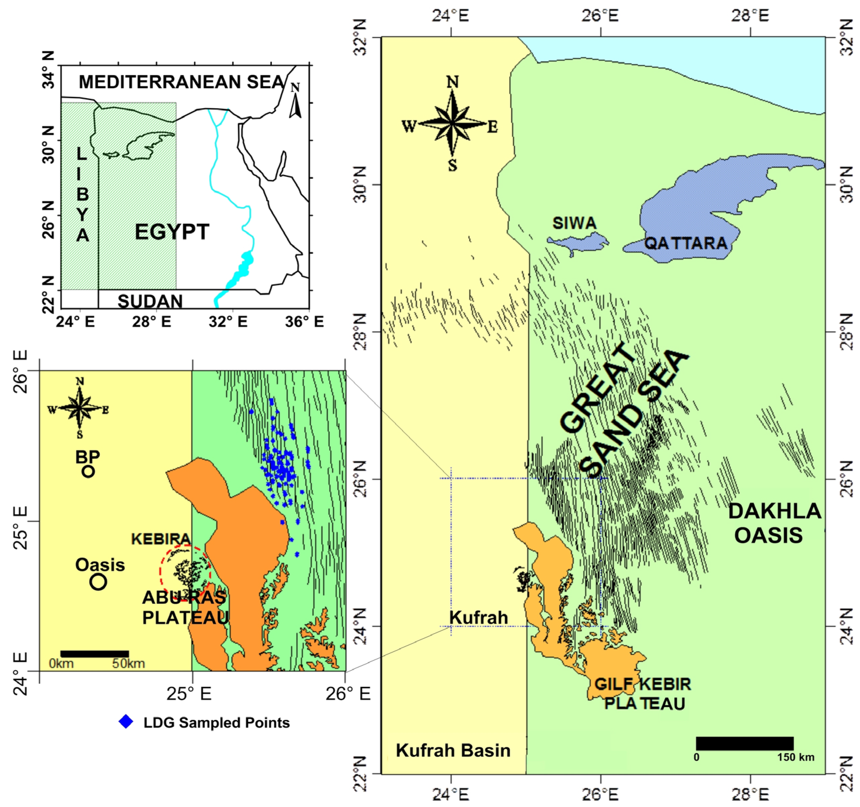
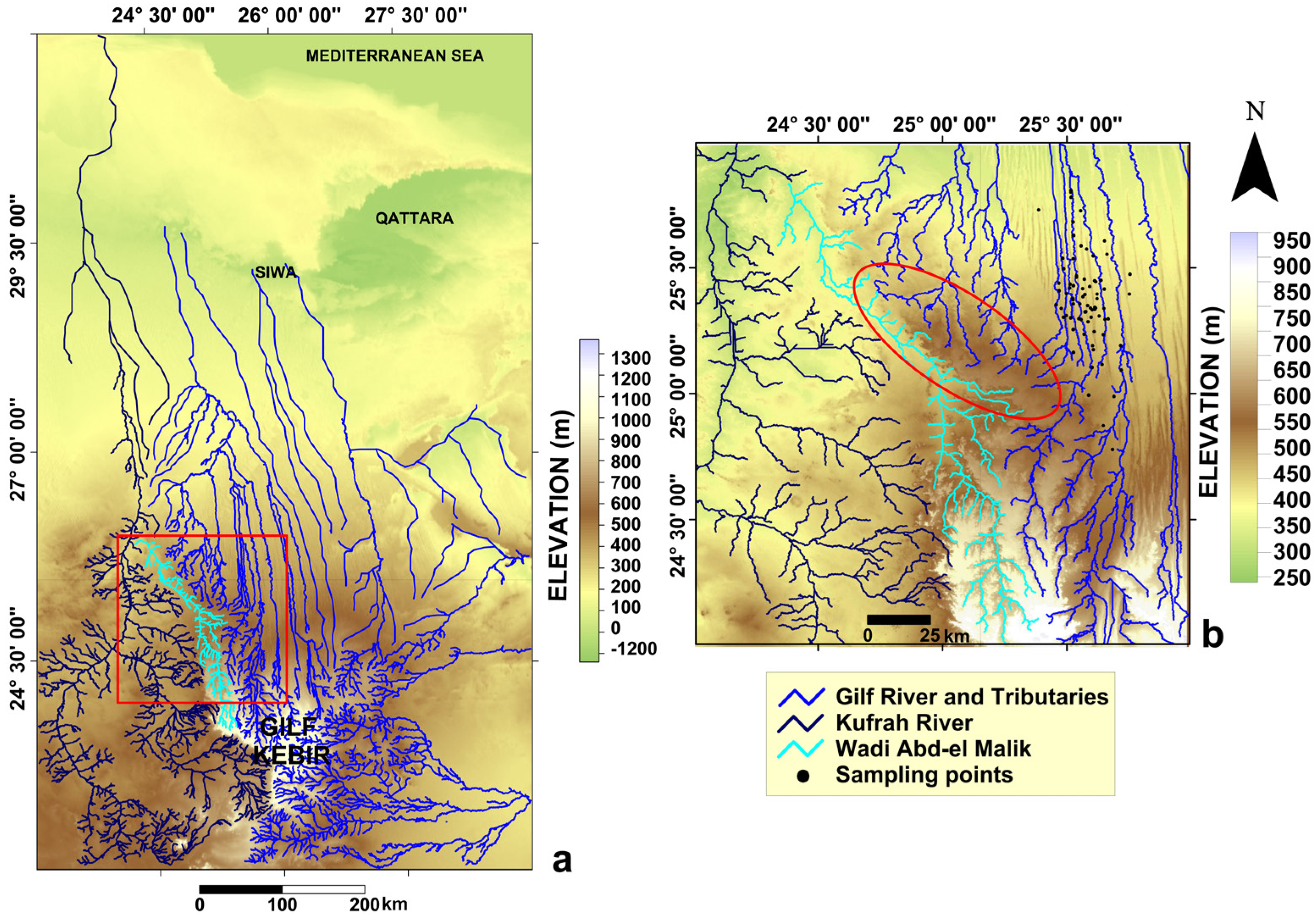
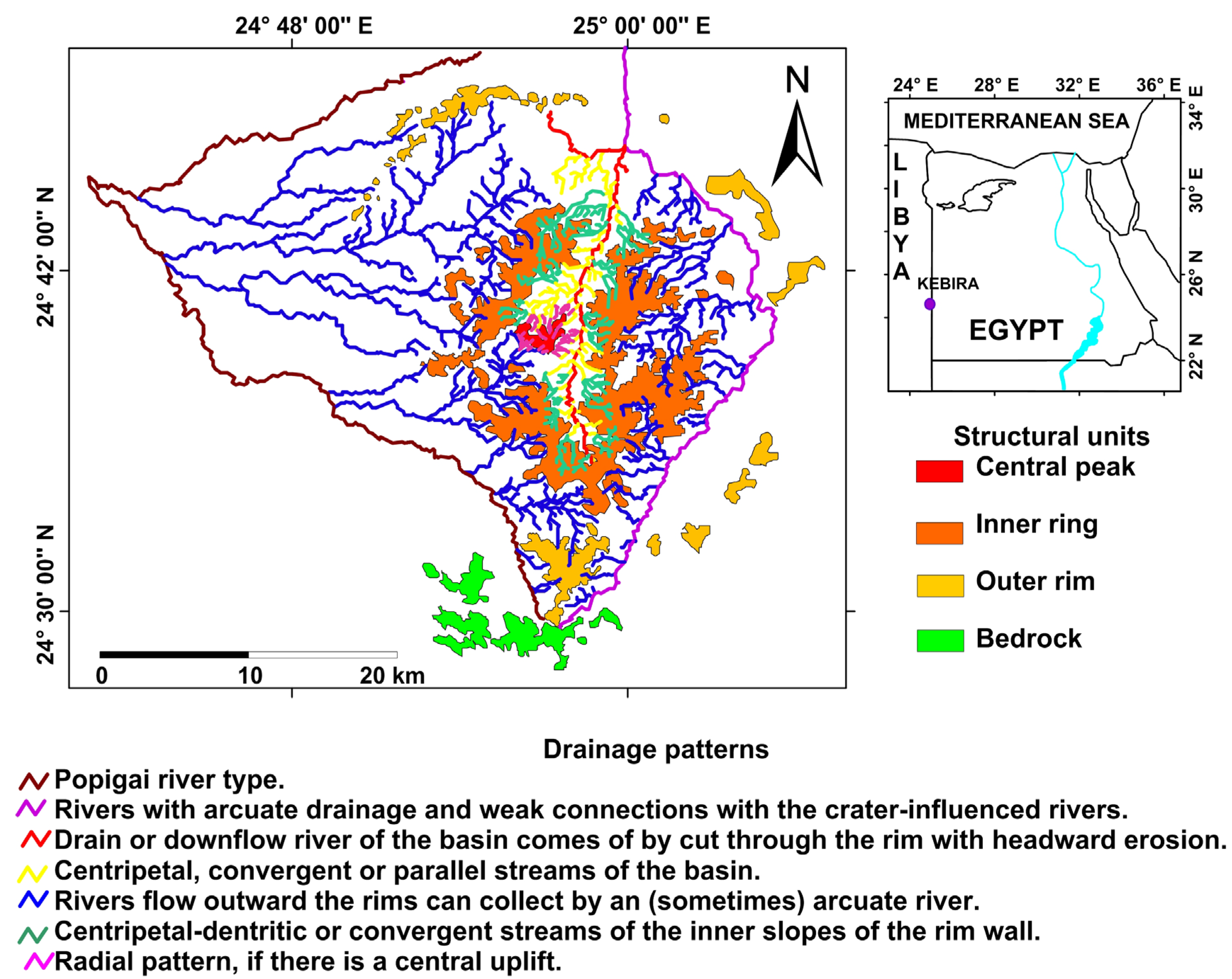
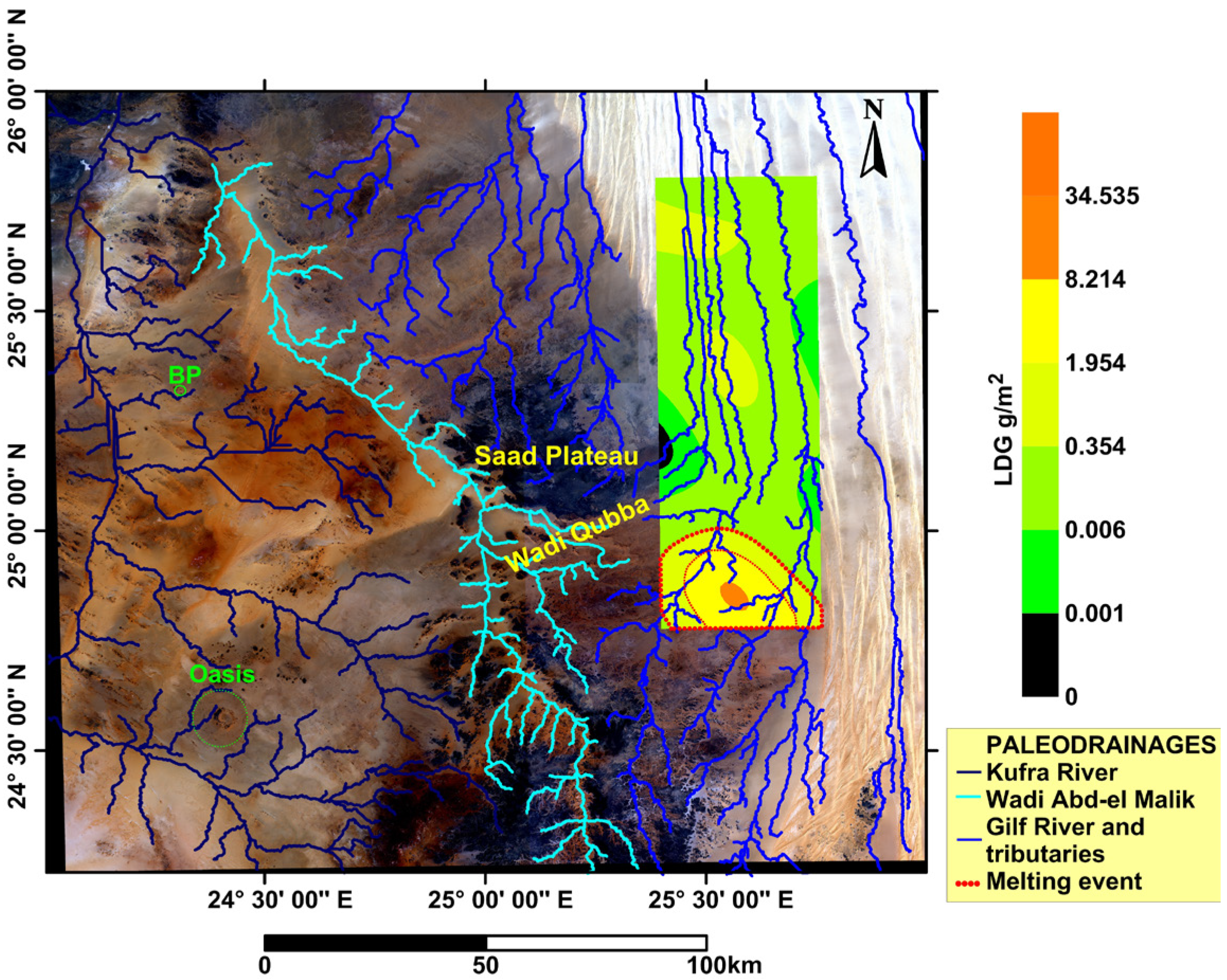
2. Study Area


3. Methods of Geostatistical Study
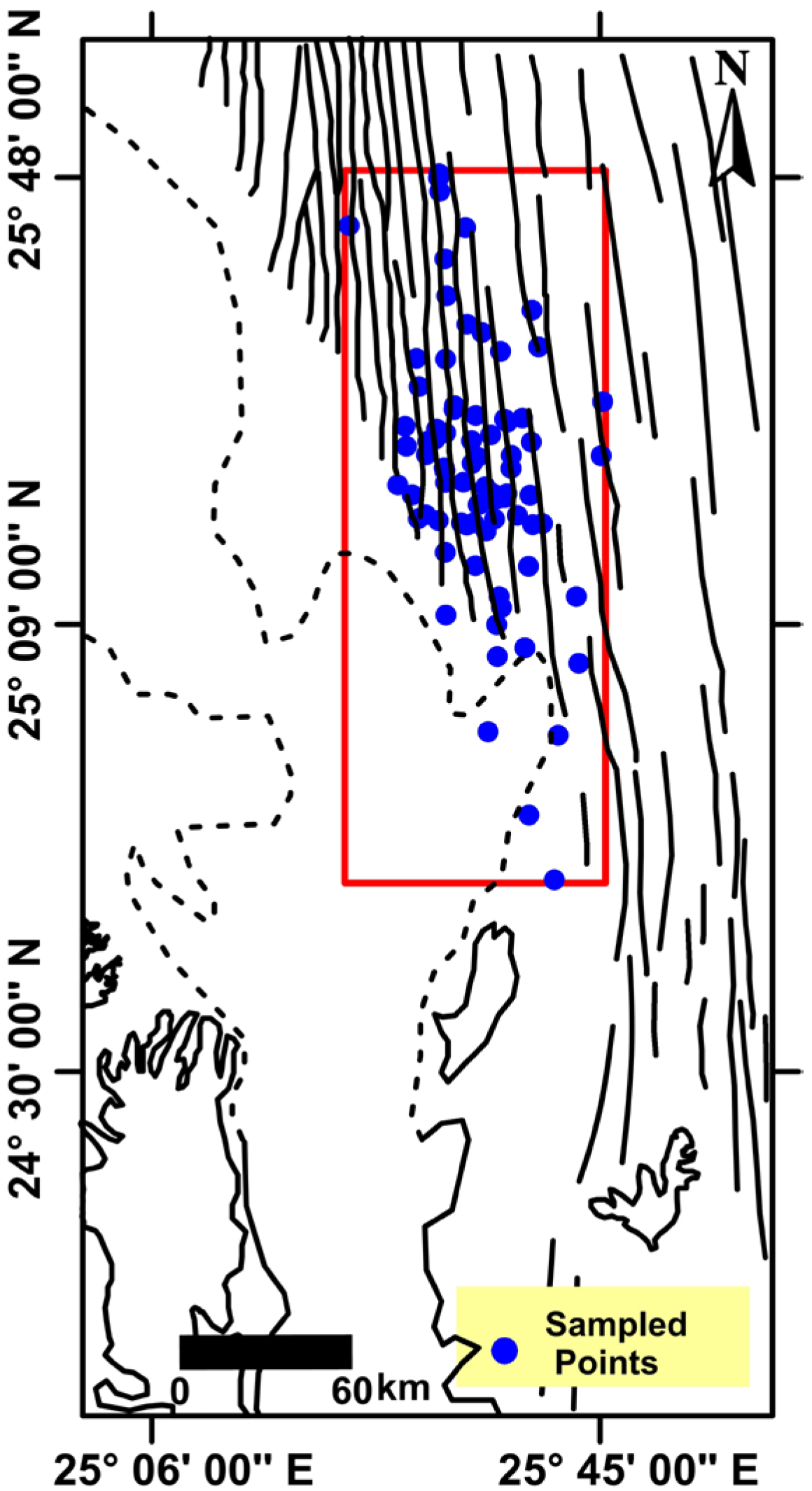
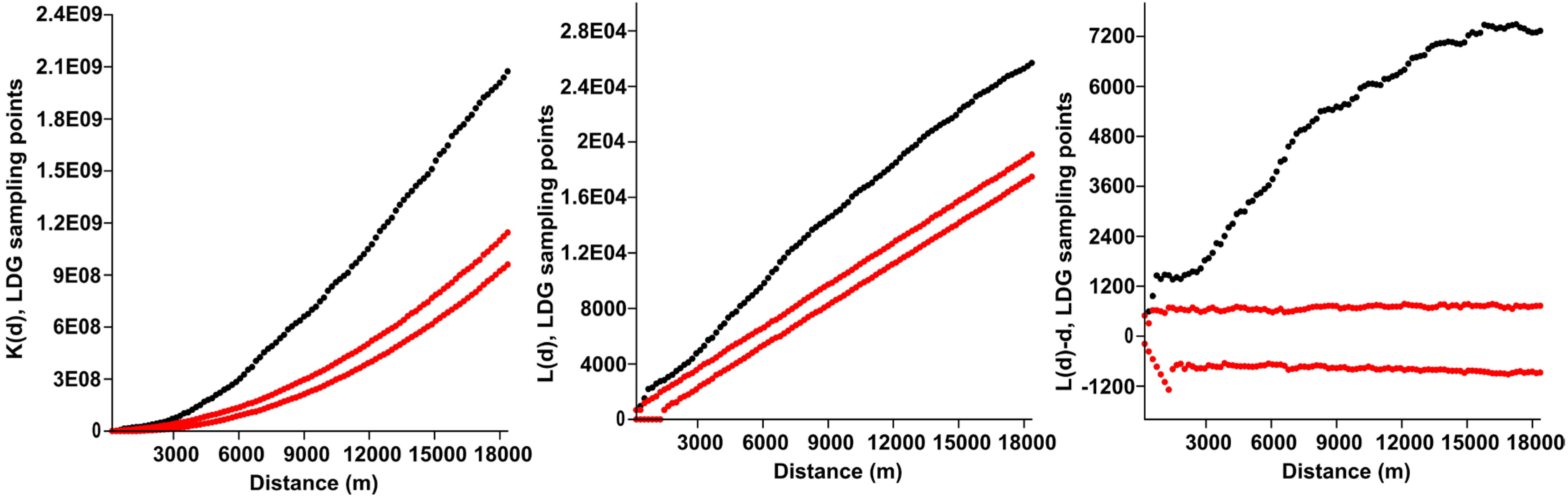
3.1. Sampling and Pattern of Univariate Data


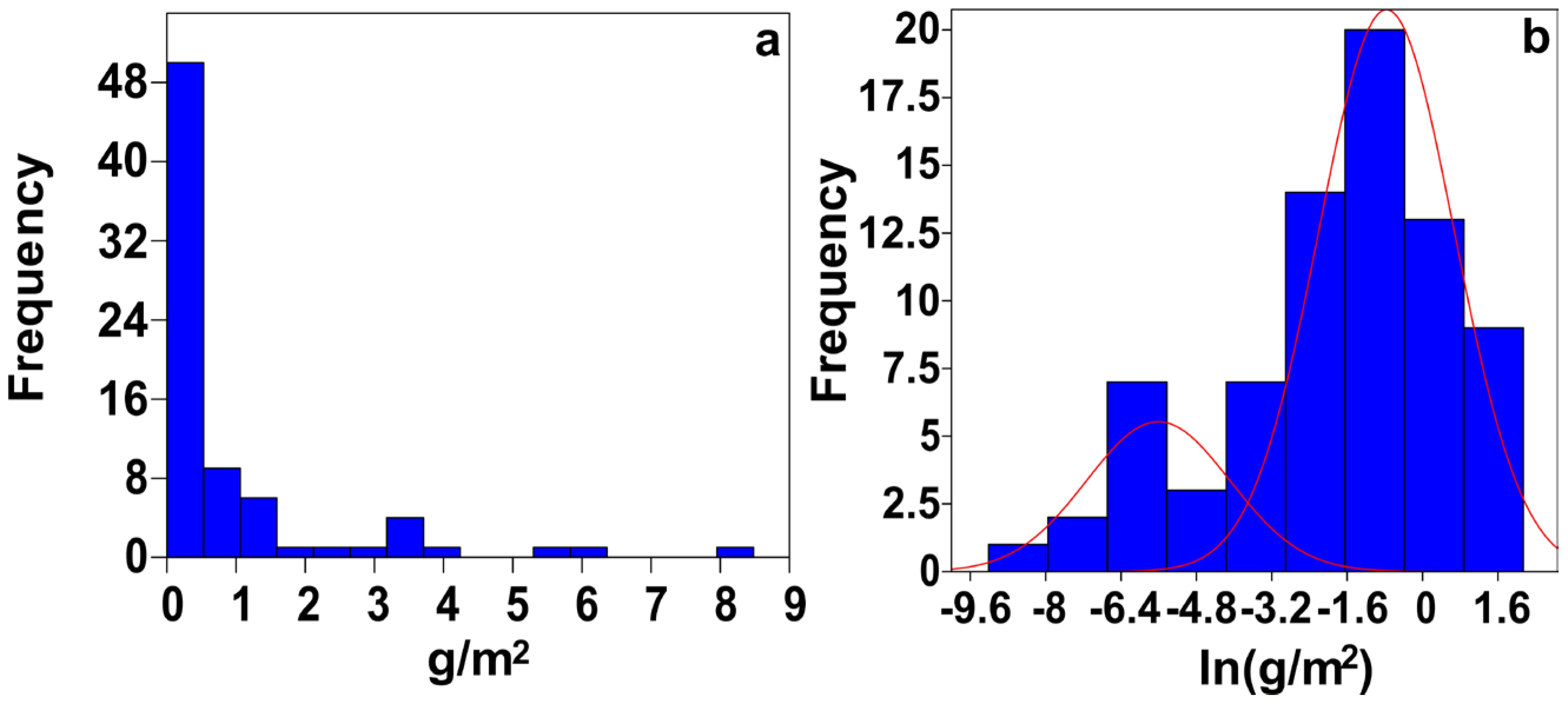
3.2. Exploratory Statistics


| Population | Probability | Mean | Standard Deviation |
|---|---|---|---|
| 1 | 0.22055 | −5.6089 | 1.5233 |
| 2 | 0.77945 | −0.76634 | 1.4361 |
| Normality Test | Original Distribution | Logarithmic-Transformed Distribution | Minor Mass Population | Major Mass Population |
|---|---|---|---|---|
| N (number of data) | 76 | 76 | 18 | 58 |
| Shapiro–Wilk W | 0.6079 | 0.9411 | 0.9119 | 0.9795 |
| p (normal) | 6.16 × 10⁻¹³ | 0.001534 | 0.09297 | 0.4313 |
| Jarque–Bera (JB) | 327.5 | 7.586 | 1.186 | 1.49 |
| p (normal) | 7.65× 10−72 | 0.02253 | 0.5528 | 0.4748 |
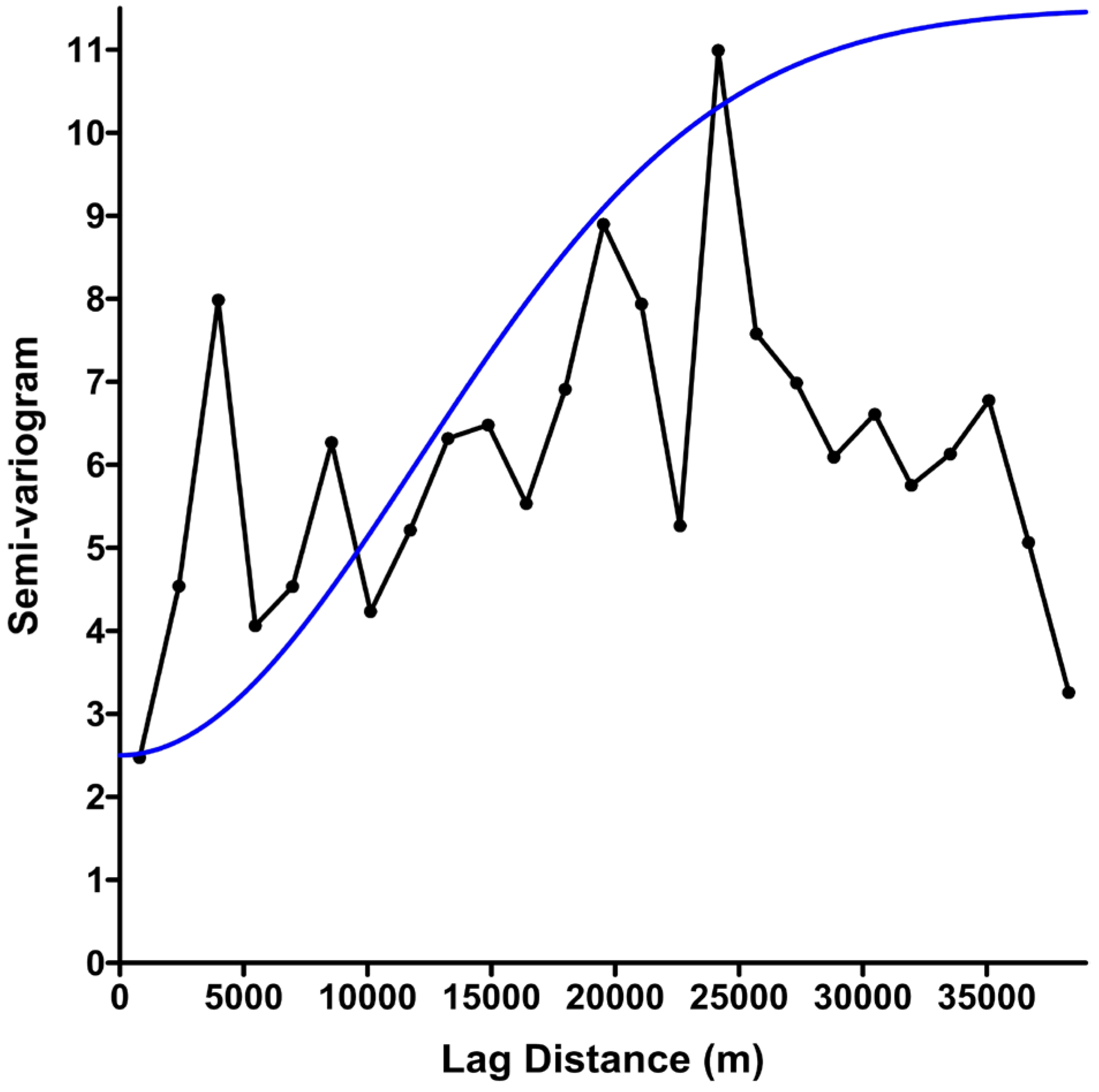
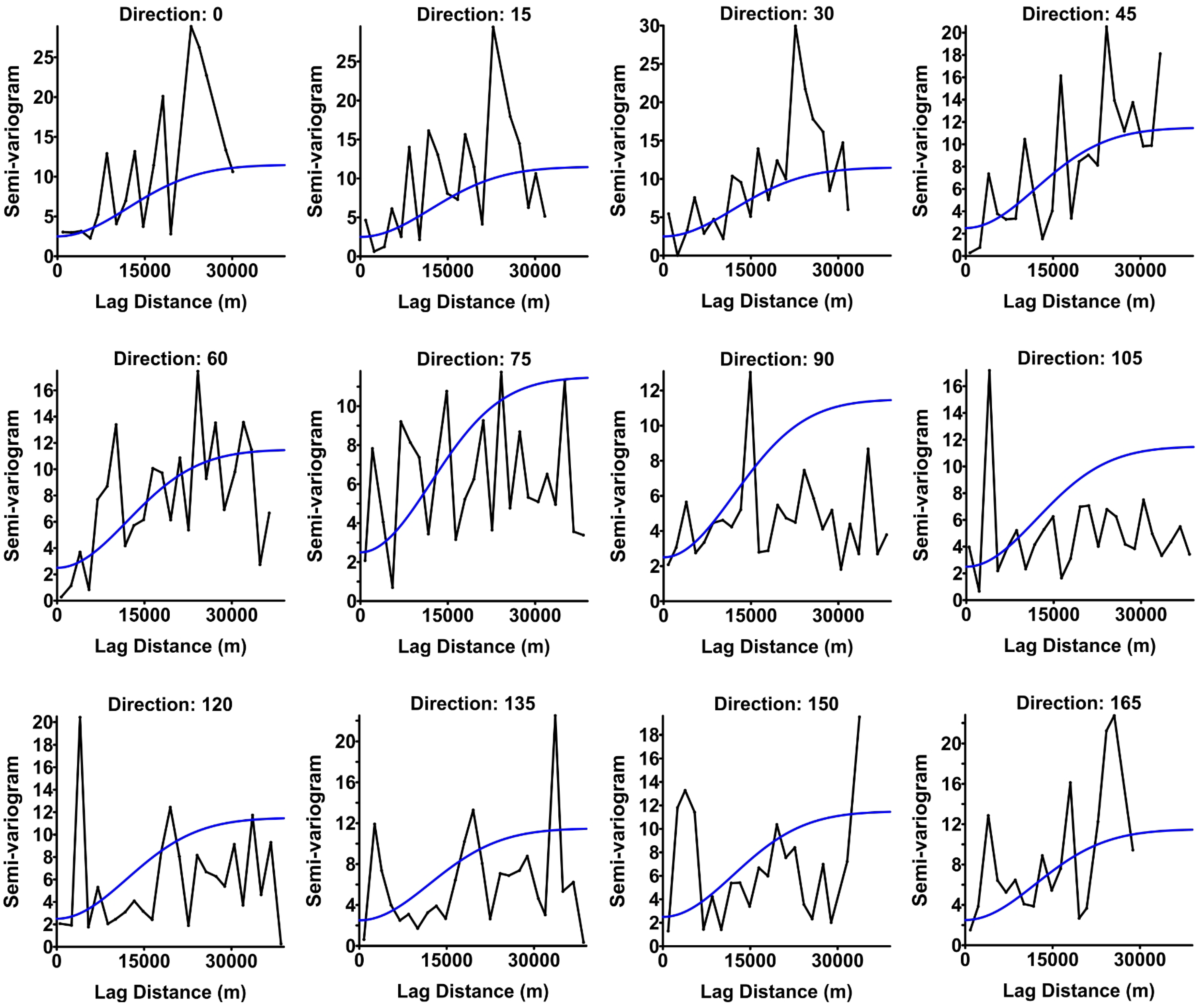
3.3. Kriging Methods
4. Digital Tools on Image Processing
- Preparation of the Digital Elevation Model (DEM).
- Elimination of the sinks. In order to obtain a “corrected DEM” for subsequent analysis, this function identifies depressed zones and fills them.
- Flux direction. The algorithm D8 traces the flow from every pixel of the DEM to one of the surrounding pixels. The result is the generation of flux lines that appear as lines perpendicular to the elevation contours.
- Determination of a raster with flow accumulation within each downslope cell. It is a calculation of the number of cells that flows into a particular downslope cell, according to flux direction [54].
- The paleodrainage network is a shape that results from the combination of the flux direction and accumulation layers by means of extension basin 1 [53].
5. Results and Discussion
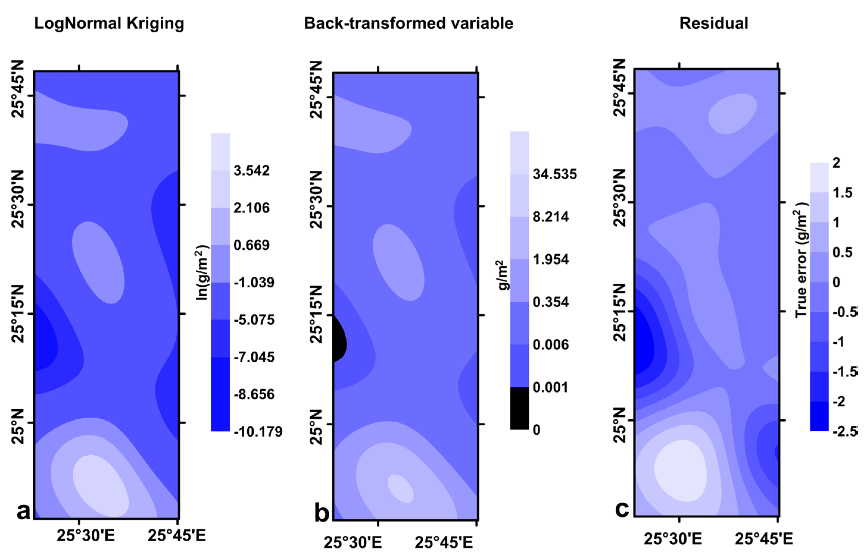
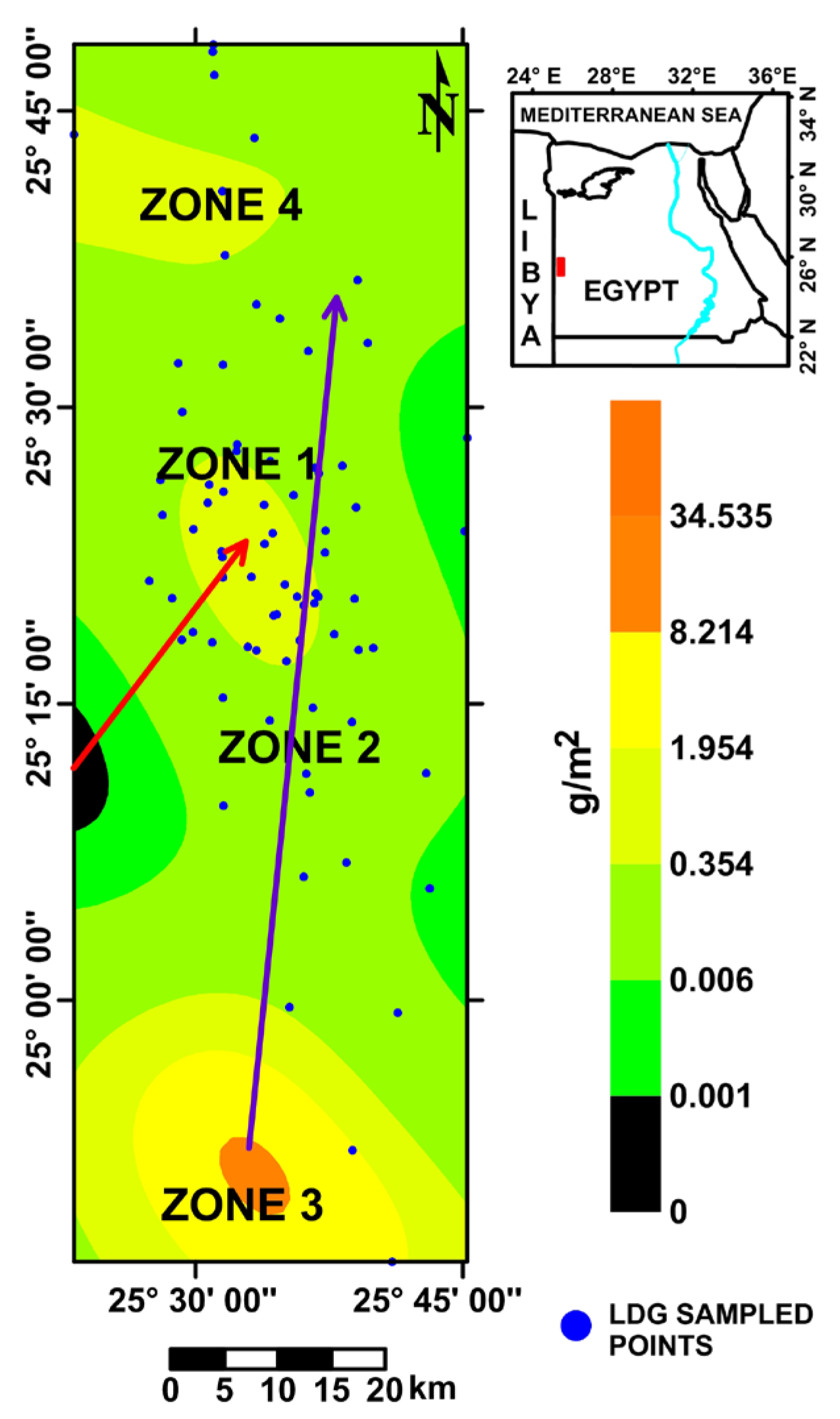
5.1. Geostatistical Mapping


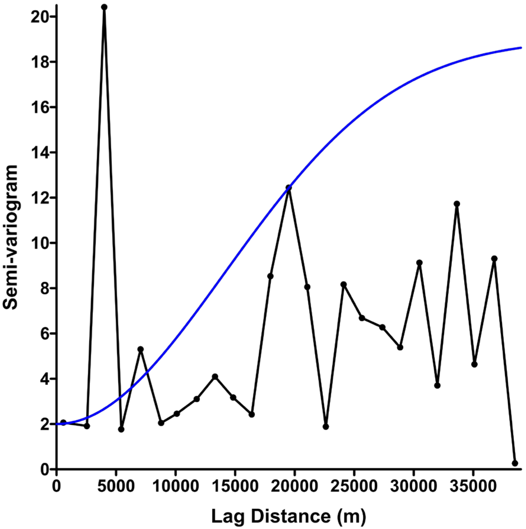
| Parameter | Omnidirectional Semi-Variogram | Final Semi-Variogram |
|---|---|---|
| Nugget effect | 2.5 | 2 |
| Sill | 9.0 | 17 |
| Range (m) | 17,000 | 20,000 |
| Nugget-sill-ratio | 0.28 | 0.12 |
| Anisotropy direction (sexagesimal degrees) from E–W | - | 30° |
| Direction of variogram (sexagesimal degrees) from E–W | - | 120° |

5.2. Understanding the Surface Distribution Model of LDG


| Population | Mean (g/m2) | Approximated Area (m2) | LDG Mass (g) |
|---|---|---|---|
| 1 | 0.004 | 3.420 × 10⁸ | 1.368 × 10⁶ |
| 2 | 0.465 | 1.082 × 10⁹ | 5.031 × 10⁸ |
| Mixture | 0.235 | 2.731 × 10⁹ | 6.404 × 10⁸ |
| Total mass | 1.145 × 10⁹ |
6. Conclusions
Acknowledgments
Author Contributions
Conflicts of Interest
References
- Matsubara, K.; Matsuda, J.; Koeberl, C. Noble gases and K-Ar ages in Aouelloul, Zhamanshin and Libyan Desert impact glasses. Geochim. Cosmochim. Acta 1991, 55, 2951–2955. [Google Scholar] [CrossRef]
- Horn, P.; Müller-Sohnius, D.; Schaaf, P.; Kleinmann, B.; Storzer, D. Potassium-argon and fission-track dating of Libyan Desert Glass, and strontium-and neodymium isotope constraints on its source rocks. In Silica ‘96, Proceedings of the Meeting on Libyan Desert Glass and Related Desert Events, Bologna, Italy, 18 July 1996; de Michele, V., Ed.; Pyramids: Segrate, Italy, 1997; pp. 59–73. [Google Scholar]
- Schaaf, P.; Müller-Sohnius, D. Strontium and neodymium isotopic study of Libyan Desert Glass: Inherited Pan-African ages signatures and new evidence for target material. Meteorit. Planet. Sci. 2002, 37, 565–576. [Google Scholar] [CrossRef]
- Albritton, C.C., Jr.; Brooks, J.E.; Issawi, B.; Swedan, A. Origin of the Qattara Depression, Egypt. Geol. Soc. Am. Bull. 1990, 102, 952–960. [Google Scholar] [CrossRef]
- Gindy, A.R.; Albritton, C.C., Jr.; Brooks, J.E.; Issawi, B.; Swedan, A. Origin of the Qattara Depression, Egypt: Discussion and reply. Geol. Soc. Am. Bull. 1991, 103, 1374–1376. [Google Scholar] [CrossRef]
- Clayton, P.A. The western side of the Gilf Kebir. Geogr. J. 1933, 81, 254–259. [Google Scholar] [CrossRef]
- Clayton, P.A.; Spencer, L.J. Silica-glass from the Libyan Desert. Mineral. Mag. 1934, 23, 501–508. [Google Scholar] [CrossRef]
- Spencer, L.J. Tektites and silica-glass. Mineral. Mag. 1939, 25, 425–440. [Google Scholar] [CrossRef]
- Weeks, R.A.; Underwood, J.R., Jr.; Giegengack, R. Libyan Desert Glass: A review. J. Non-Cryst. Solids 1984, 67, 593–619. [Google Scholar] [CrossRef]
- Barakat, A.A.; de Michele, V.; Negro, G.; Piacenza, B.; Serra, R. Some new data on the distribution of Libyan Desert Glass (Great Sand Sea, Egypt). In Silica ‘96, Proceedings of the Meeting on Libyan Desert Glass and Related Desert Events, Bologna, Italy, 18 July 1996; de Michele, V., Ed.; Pyramids: Segrate, Italy, 1997; pp. 29–36. [Google Scholar]
- Tilton, G.R. Isotopic composition of lead from tektites. Geochim. Cosmochim. Acta 1958, 14, 323–330. [Google Scholar] [CrossRef]
- Faul, H. Tektites are terrestrial. Science 1966, 152, 1341–1345. [Google Scholar] [CrossRef] [PubMed]
- Yiou, F.; Ruisbeck, G.M.; Klein, J.; Middleton, R. 26Al/10Be in terrestrial impact glasses. J. Non-Cryst. Solids 1984, 67, 503–509. [Google Scholar] [CrossRef]
- Koeberl, C.; Kluger, F.; Kiesl, W. Rare earth element determination at ultratrace abundance levels in geological materials. J. Radioanal. Nucl. Chem. 1987, 112, 481–487. [Google Scholar] [CrossRef]
- Murali, A.V.; Zolensky, M.E.; Underwood, J.R., Jr.; Giegengack, R. Chondritic debris in Libyan Desert Glass . In Silica ‘96, Proceedings of the Meeting on Libyan Desert Glass and Related Desert Events; Bologna, Italy, 18 July 1996, de Michele, V., Ed.; Pyramids: Segrate, Italy, 1997; pp. 133–142. [Google Scholar]
- Koeberl, C. Libyan Desert Glass: Geochemical composition and origin. In Silica ‘96, Proceedings of the Meeting on Libyan Desert Glass and Related Desert Events, Bologna, Italy, 18 July 1996; de Michele, V., Ed.; Pyramids: Segrate, Italy, 1997; pp. 121–131. [Google Scholar]
- Barrat, J.A.; Jahn, B.M.; Amossé, J.; Rocchia, R.; Keller, F.; Poupeau, G.R.; Diemer, E. Geochemistry and origin of Libyan Desert glasses. Geochim. Cosmochim. Acta 1997, 61, 1953–1959. [Google Scholar] [CrossRef]
- Koeberl, C. Confirmation of a meteoritic component in Libyan Desert Glass from osmium isotopic data. In Proceedings of the 63th Annual Meeting of the Meteoritical Society, Chicago, IL, USA, 28 August–1 September 2000. Abstract #5253.
- Moynier, F.; Beck, P.; Jourdan, F.; Yin, Q.-Z.; Reimold, U.; Koeberl, C. Isotopic fractionation of zinc in tektites. Earth Planet. Sci. Lett. 2009, 277, 482–489. [Google Scholar] [CrossRef]
- Magna, T.; Deutsch, A.; Mezger, K.; Skála, R.; Seitz, H.M.; Mizera, J.; Řanda, Z.; Adolph, L. Lithium in tektites and impact glasses: Implications for sources, histories and large impacts. Geochim. Cosmochim. Acta 2011, 75, 2137–2158. [Google Scholar] [CrossRef]
- Kleinmann, B. The breakdown of zircon observed in the Libyan Desert Glass as evidence of its impact origin. Earth Planet. Sci. Lett. 1968, 5, 497–501. [Google Scholar] [CrossRef]
- Murali, A.V.; Zolensky, M.E.; Underwood, J.R., Jr.; Giegengack, R.F. Formation of Libyan Desert Glass. In Proceedings of the 19th Lunar and Planetary Science Conference, Houston, TX, USA, 14–18 March 1988; pp. 817–818.
- Storzer, D.; Koeberl, C. Uranium and Zirconium Enrichments in Libyan Desert Glass: Zircon Baddeleyite and High Temperature History of the Glass. In Proceedings of the 22th Lunar and Planetary Science Conference, Houston, TX, USA, 18–22 March 1991; pp. 1345–1346.
- Kramers, J.D.; Andreoli, M.A.G.; Atanasova, M.; Belyanin, G.A.; Block, D.L.; Franklyn, C.; Harris, C.; Lekgoathi, M.; Montross, C.S.; Ntsoane, T.; Pischedda, V.; Segonyane, P.; Viljoen, K.S.; Westraadt, J.E. Unique chemistry of a diamond-bearing pebble from the Libyan Desert Glass strewnfield, SW Egypt: Evidence for a shocked comet fragment. Earth Planet. Sci. Lett. 2013, 382, 21–31. [Google Scholar] [CrossRef]
- Boslough, M.B.E.; Crawford, D.A. Low-altitude airbursts and the impact threat. Int. J. Impact Eng. 2008, 35, 1441–1448. [Google Scholar] [CrossRef]
- Wasson, J.T. Large aerial bursts: An important class of terrestrial accretionary events. Astrobiology 2003, 3, 163–179. [Google Scholar] [CrossRef] [PubMed]
- Abate, B.; Koeberl, C.; Kruger, F.J.; Underwood, J.R., Jr. BP and Oasis impact structures, Libya, and their relation to Libyan Desert Glass. In Large Meteorite Impacts and Planetary Evolution II; Special Papers Volume 339; Dressler, B.O., Sharpton, V.L., Eds.; Geological Society of America: Boulder, CO, USA, 1999; pp. 177–192. [Google Scholar]
- Koeberl, C.; Reimold, W.U.; Plescia, J. BP and Oasis impact structures, Libya: Remote Sensing and Field Studies. In Impact Tectonics; Koeberl, C., Henkel, H., Eds.; Springer-Verlag: Berlin, Germany, 2005; pp. 161–190. [Google Scholar]
- El-Baz, F.; Ghoneim, E. Largest crater shape in the Great Sahara revealed by multispectral images and radar data. Int. J. Remote Sens. 2007, 28, 451–458. [Google Scholar] [CrossRef]
- Aboud, T. Libyan Desert Glass: Has the enigma of its origin been resolved? Phys. Procedia 2009, 2, 1425–1432. [Google Scholar] [CrossRef]
- Paillou, P.; El Barkooky, A.; Barakat, A.; Malezieux, J.-M.; Reynard, B.; Dejax, J.; Heggy, E. Discovery of the largest impact crater field on Earth in the Gilf Kebir region, Egypt. Comptes Rendus Geosci. 2004, 336, 1491–1500. [Google Scholar] [CrossRef]
- Orti, L.; Di Martino, M.; Morelli, M.; Cigolini, C.; Pandeli, E.; Buzzigoli, A. Non-impact origin of the crater-like structures in the Gilf Kebir area (Egypt): Implications for the geology of eastern Sahara. Meteorit. Planet. Sci. 2008, 43, 1629–1639. [Google Scholar] [CrossRef]
- Paillou, P.; Reynard, B.; Malezieux, J.-M.; Dejax, J.; Heggy, E.; Rochette, P.; Reimold, W.U.; Michel, P.; Baratoux, D.; Razin, P.; Colin, J.-P. An extended field of crater-shaped structures in the Gilf Kebir region, Egypt: Observations and hypotheses about their origin. J. Afr. Earth Sci. 2006, 6, 281–299. [Google Scholar] [CrossRef]
- Ramirez-Cardona, M.; El-Barkooky, A.; Hamdan, M.; Flores-Castro, K.; Jiménez-Martínez, N.I.; Mendoza-Espinosa, M. On the Libyan Desert Silica Glass (LDSG) transport model from a hypothetical impact structure. In Proceedings of the 33th International Geological Congress, Oslo, Norway, 6–14 August 2008.
- Issawi, B.; McCauley, J.F. The Cenozoic rivers of Egypt: The Nile problem. In The Followers of Horus; Egyptian Studies Association Publication No. 2, Oxbow Monograph 20; Friedman, R., Adams, B., Eds.; Oxbow Books: Oxford, UK, 1992; pp. 121–138. [Google Scholar]
- Sampsell, B.M. A Traveler’s Guide to the Geology of Egypt; The American University in Cairo Press: Cairo, Egypt, 2003; p. 140. [Google Scholar]
- Klitzsch, E.; Harms, J.C.; Lejal-Nicol, A.; List, F.K. Major subdivisions and depositional environments of Nubia strata, southwestern Egypt. AAPG Bull. 1979, 63, 967–974. [Google Scholar]
- Tawadros, E.E. Geology of North Africa; CRC Press/Balkema: Leiden, The Netherlands, 2012; pp. 202–203. [Google Scholar]
- Myers, D.E. To be or not to be…Stationary? That is the question. Math. Geol. 1989, 21, 347–362. [Google Scholar] [CrossRef]
- Ripley, B.D. Tests of ‘randomness’ for spatial point patterns. J. R. Stat. Soc. B. 1979, 41, 368–374. [Google Scholar]
- Davis, J.C. Statistics and Data Analysis in Geology, 3rd ed.; John Wiley & Sons: New York, NY, USA, 2002; pp. 310–313. [Google Scholar]
- Dixon, P.M. Ripley’s K function. In Encyclopedia of Environmetrics; El-Shaarawi, A.H., Piegorsch, W.W., Eds.; John Wiley & Sons: New York, NY, USA, 2002; Volume 3, pp. 1796–1803. [Google Scholar]
- Hammer, Ø.; Harper, D.A.T.; Ryan, P.D. PAST: Paleontological Statistics Software Package for Education and Data Analysis. Palaeontol. Electron. 2001, 4, 1–9. [Google Scholar]
- Dempster, A.P.; Laird, N.M.; Rubin, D.B. Maximum likelihood from incomplete data via the EM algorithm. J. R. Stat. Soc. B. 1977, 39, 1–38. [Google Scholar]
- Shapiro, S.S.; Wilk, M.B. An analysis of variance test for normality (complete samples). Biometrika 1965, 52, 591–611. [Google Scholar] [CrossRef]
- Jarque, C.M.; Bera, A.K. A test for normality of observations and regression residuals. Int. Stat. Rev. 1987, 55, 163–172. [Google Scholar] [CrossRef]
- Journel, A.G. The lognormal approach to predicting local distribution of selective mining unit grades. Math. Geol. 1980, 12, 285–303. [Google Scholar] [CrossRef]
- Yamamoto, J.K. On unbiased backtransform of lognormal kriging estimates. Comput. Geosci. 2007, 11, 219–234. [Google Scholar] [CrossRef]
- Yamamoto, J.K. Correcting the Smoothing Effect of Ordinary Kriging Estimates. Math. Geol. 2005, 37, 69–94. [Google Scholar] [CrossRef]
- Mihályi, K.; Gucsik, A.; Szabó, J. Drainage patterns of terrestrial complex meteorite craters: A hydrogeological overview. In Proceedings of the 39th Lunar and Planetary Science Conference, League City, TX, USA, 10–14 March 2008. Abstract #1200.
- Fairfield, J.; Leymarie, P. Drainage networks from grid digital elevation models. Water Resour. Res. 1991, 27, 709–717. [Google Scholar] [CrossRef]
- Digital Elevation Model (DEM) tiles from Shuttle Radar Topography Mission (SRTM) data. Available online: ftp://e0srp01u.ecs.nasa.gov/srtm/version2/SRTM3/Africa (accessed on 10 January 2010).
- Petras, I. “Basin1” ArcView GIS Extension. Available online: http://arcscripts.esri.com (accessed on 7 January 2008).
- Maza, J. Hydro ArcView GIS Extension. Available online: http://haciendomapas.blogspot.com (accessed on 7 January 2008).
- Paillou, P.; Schuster, M.; Tooth, S.; Farr, T.; Rosenqvist, A.; Lopez, S.; Malezieux, J.-M. Mapping of a major paleodrainage system in eastern Libya using orbital imaging radar: The Kufra River. Earth Planet. Sci. Lett. 2009, 277, 327–333. [Google Scholar] [CrossRef]
- Robinson, C.A.; Werwer, A.; El-Baz, F.; El-Shazly, M.; Fritch, T.; Kusky, T. Nubian Aquifer in Southwest Egypt. Hydrogeol. J. 2007, 15, 33–45. [Google Scholar] [CrossRef]
- Ferrière, L.; Devouard, B.; Goderis, S.; Vincent, P.; Bernon, D.; Lorillard, R.; Saul, J.M. Petrographic and geochemical study of an anomalous melt rock from the Gilf Kebir Plateau, close to the Libyan Desert Glass area, Egypt. In Proceedings of the 72nd Annual Meeting of the Meteoritical Society, Nancy, France, 13–18 July 2009. Abstract #5384.
- Artemieva, N.; Pierazzo, E.; Stöffler, D. Numerical modeling of tektite origin in oblique impacts: Implication to Ries-Moldavites strewn field. Bull. Geosci. 2002, 77, 303–311. [Google Scholar]
- Artemieva, N. Numerical modeling of the Australasian tektite strewn field. In Proceedings of the 44th Lunar and Planetary Science Conference, The Woodlands, TX, USA, 18–22 March 2013. Abstract #1410.
© 2015 by the authors; licensee MDPI, Basel, Switzerland. This article is an open access article distributed under the terms and conditions of the Creative Commons Attribution license (http://creativecommons.org/licenses/by/4.0/).
Share and Cite
Jimenez-Martinez, N.; Ramirez, M.; Diaz-Hernandez, R.; Rodriguez-Gomez, G. Fluvial Transport Model from Spatial Distribution Analysis of Libyan Desert Glass Mass on the Great Sand Sea (Southwest Egypt): Clues to Primary Glass Distribution. Geosciences 2015, 5, 95-116. https://0-doi-org.brum.beds.ac.uk/10.3390/geosciences5020095
Jimenez-Martinez N, Ramirez M, Diaz-Hernandez R, Rodriguez-Gomez G. Fluvial Transport Model from Spatial Distribution Analysis of Libyan Desert Glass Mass on the Great Sand Sea (Southwest Egypt): Clues to Primary Glass Distribution. Geosciences. 2015; 5(2):95-116. https://0-doi-org.brum.beds.ac.uk/10.3390/geosciences5020095
Chicago/Turabian StyleJimenez-Martinez, Nancy, Marius Ramirez, Raquel Diaz-Hernandez, and Gustavo Rodriguez-Gomez. 2015. "Fluvial Transport Model from Spatial Distribution Analysis of Libyan Desert Glass Mass on the Great Sand Sea (Southwest Egypt): Clues to Primary Glass Distribution" Geosciences 5, no. 2: 95-116. https://0-doi-org.brum.beds.ac.uk/10.3390/geosciences5020095