A Spatial Pattern Analysis of Frontier Passes in China’s Northern Silk Road Region Using a Scale Optimization BLR Archaeological Predictive Model

Abstract

In China’s Northern Silk Road (CNSR) region, dozens of frontier passes built and fortified at critical intersections were exploited starting at approximately 114 B.C. to guarantee caravan safety. Understanding the pattern of these pass sites is helpful in understanding the defense and trading system along the Silk Road. In this study, a scale optimization Binary Logistic Regression (BLR) archaeological predictive model was proposed to study the spatial pattern of CNSR frontier passes for understanding the critical placement of ancient defense and trading pass sites. Three hundred and fifty sample locations and 17 natural proxies were input into the model. Four strongly correlated factors were reserved as independent variables to construct the model, which was validated by 150 surveyed data and Kvamme’s Gain statistics. According to the variable selection and model optimization, the best spatial scale varies with the stability of the variables, such as 50 m and 1000 m, respectively, for the terrain and non-terrain variables. Clustering characteristics were identified with division overlapped with a 400 mm precipitation line using the site sensibility map. The high and medium probability areas were assembled along the Great Wall and the CNSR routes, especially in the western part, revealing that the model is also helpful to reconstruct the Silk Road routes.

1. Introduction

Frontier passes are strategically situated and difficult to access. They are typically built on ancient borders or ancient critical intersections, fortified, and guarded by troops. During the cold weapon era, which includes the Chinese Shang (1600–1046 B.C.) to Song (960–1279 A.D.) dynasties, hundreds of impregnable frontier passes, including fortified mountain passes, Great Wall passes, barrier plugs, forts, and ferries, were constructed to defend against nomadic tribes [1]. From the start of the firearms era, particularly during the Ming Dynasty (1368–1644 A.D.), most frontier passes were renovated from defense forts into custom stations or border markets to impose trade control and taxes. The Silk Road (Seidenstraße in German), first named by the German geographer Ferdinand Freiherr von Richthofen in 1877 [2,3], consists of a series of ancient trade and cultural transmission routes that pass through regions of the Asian continent and connect the West and East, from China to the Mediterranean Sea [4]. Tens of frontier passes were built and staffed with troops in the region of China’s Northern Silk Road (CNSR) near the ancient northern frontier [5]. These passes served both to guard territory and to control trade. Today, most of these known frontier pass sites have been preserved as cultural sites and tourist attractions. In December 1987, the Great Wall—including all passes—was included in the World Heritage List [6]. On June 22, 2014, UNESCO inscribed 5000 km of the Silk Road Routes into the World Heritage list. This designated area comprises 33 sites, and includes 2 of China’s frontier pass sites (Yumen pass and Hangu pass) [7].

To protect these sites, it is essential to understand the distribution, function, and history of the frontier passes as well as their relationships to the Silk Road routes and to the Great Wall. Most previous research has focused on archaeological field work concerning frontier pass sites and archaeological detection with Visible and Infrared (VIR)/Synthetic Aperture Radar (SAR) remote sensing images, especially along the western routes [8,9,10,11]. Research is rare on whole range, large-scale pass site pattern analysis along the Silk Road.

Archaeological Predictive Models (APMs) could be applied as pattern analysis tools [12,13,14]. By establishing APMs, the occurrence probability of archaeological sites with their distribution patterns or site densities is evaluated. APMs have been successfully applied in European, Asian, and American archaeology to reveal correlations between site distribution patterns and circumstances [15,16,17,18,19,20,21,22,23,24,25,26]. In China, the application of predictive models focuses on settlement archaeology. Ni [27], Peng et al. [28], Qiao et al. [29], and Dong and Jin [30] applied a predictive model to archaeological analysis for the Shu River Basin, the Wensi Basin, Zhengluo, and the ancient Bohai state to obtain correlations between cultural remains and natural features. Given the scale and scope of China’s Northern Silk Road, APMs are helpful to provide prior information and interpretation. Thus, in this study, taking into account the advantage of the spatial analysis of APMs, an improved inductive model with scale optimization was proposed to analyse the distribution of pass sites in China’s Northern Silk Road region.

2. Study Area, Materials, and Methods

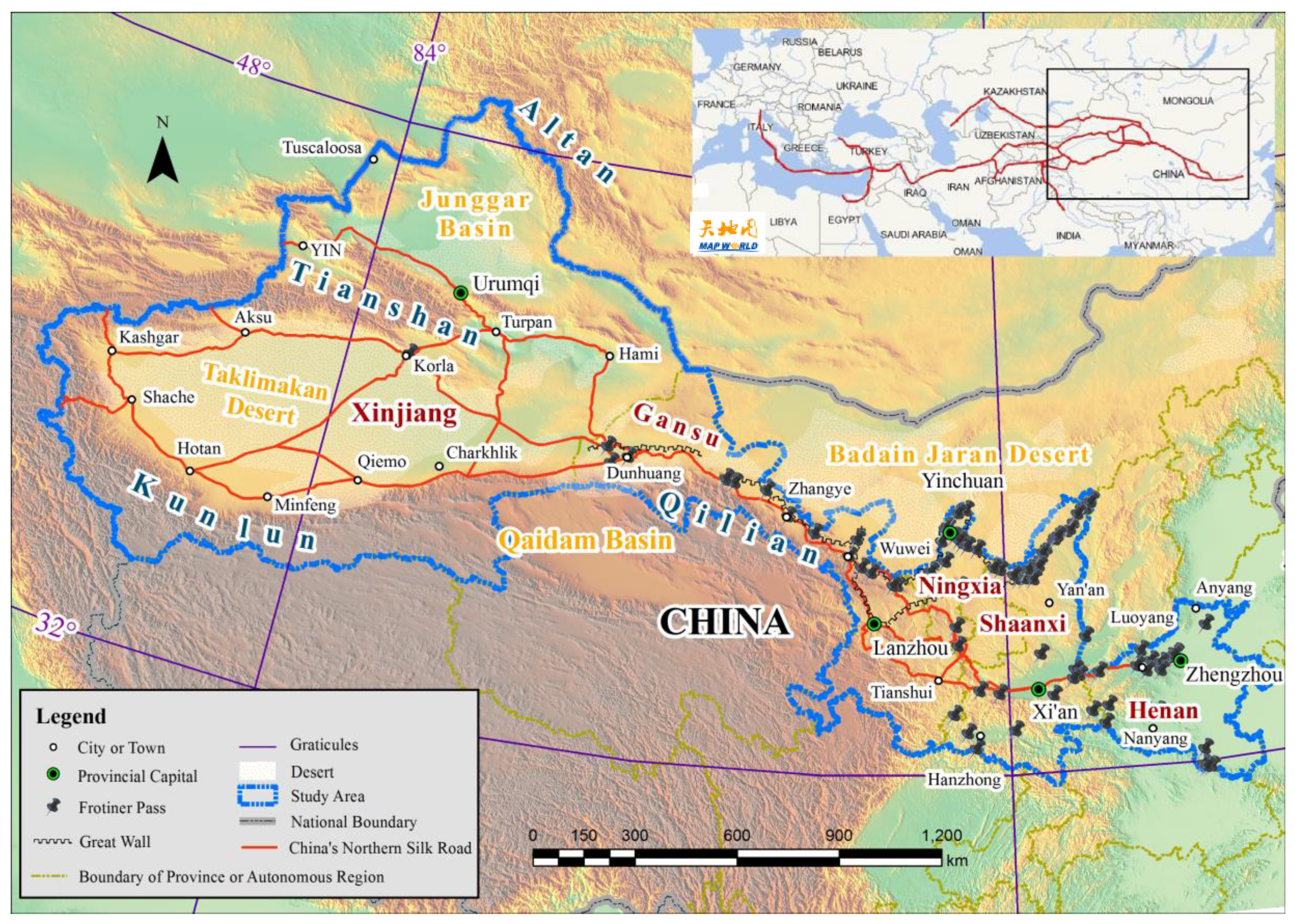
2.1. Study Area

This study focuses on the frontier pass sites along or near ancient China’s Northern Silk Road (CNSR) routes, which start from Luoyang, travel to the Loess plateau at Xi’an, pass through the Hosi Corridor along the Qilian Mountain to the Yumen pass, and then turn west. It is the eastern part of the ancient Silk Road shown in the inset map of Figure 1. The study area covers a route buffer zone that includes Henan Province, Shaanxi Province, Gansu Province, Ningxia Hui Autonomous Region, and Xinjiang Uyghur Autonomous Region, whose boundaries are located between the latitudes 31.38°–49.18° N and the longitudes 73.45°–116.64° E, covering nearly 2,553,800 km², and the altitude ranges between 600–5400 m above sea level (asl), as shown in Figure 1. This region comprises multiple landscapes: it touches great rivers, crusty salt flats, vast deserts, and snow-capped mountains. The climate varies from dry to semi-humid, while vegetation covers deserts, steppes, alpine steppes, and oases. There are plenty of world-famous archaeological sites, including historic old cities or towns, such as Chang’an, Luoyang, and Dunhuang, along the Silk Road.

2.2. Materials

Generating the database used in APMs required the collection and compilation of geographical spatial data and archaeological data, which are described below.

2.2.1. General Geographical Spatial Data

Geographical spatial data for elevation, hydrology, land cover, and soils were acquired to develop the independent variables for the model.

• Five land cover products, including the International Geosphere Biosphere Programme (IGBP) global land cover dataset (IGBP-DISCover) Version 2 [32], global land cover for the year 2000 (GLC2000) [33], the University of Maryland (UMd) land cover dataset [34], the MODerate resolution Imaging Spectroradiometer (MODIS) global land cover [35,36], and the WESTDC land cover product 2.0, as well as soil classes based on the United Nations Food and Agriculture Organization (FAO90) from the Harmonized World Soil Database (HWSD), version 1.1, were provided by the Cold and Arid Regions Science Data Centre at Lanzhou, which maintains a web portal [37] to distribute these datasets and was the source for all the geographic information system (GIS) data layers used in this research. The 30-meter Global Land Cover Dataset (GL30) collected by the National Geomatics Centre of China and Map World [38] was also explored.
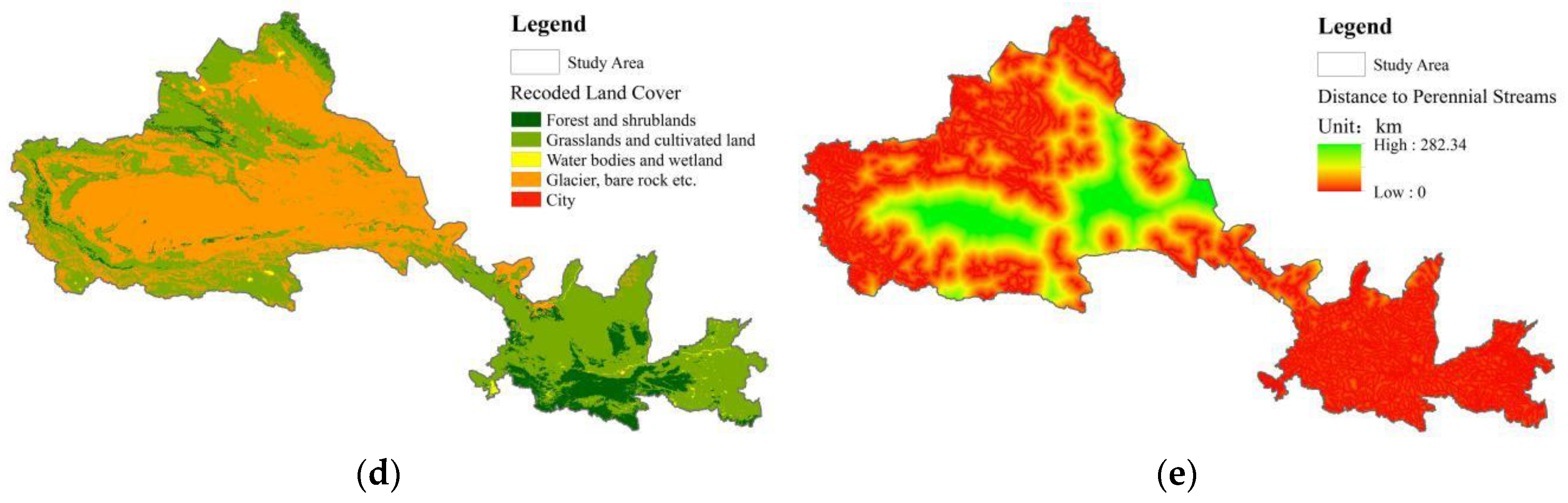
• Hydrology and administrative boundary data were extracted from 1:4,000,000 national GIS data. The intermittent and perennial stream lines from Diva data [39] were also used to analyse the impact of water on site distribution.
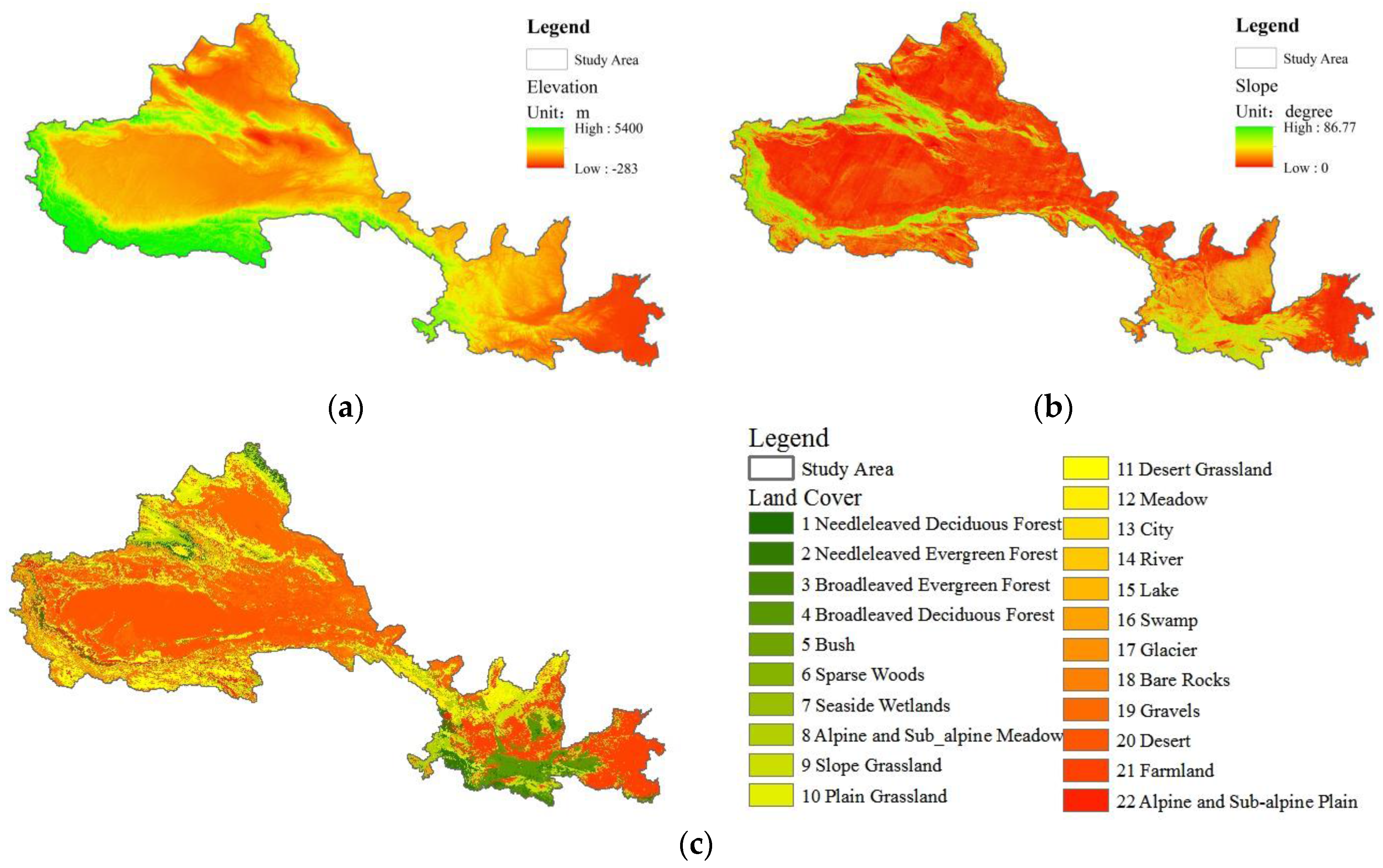
• Advanced Spaceborne Thermal Emission and Reflection Radiometer Global Digital Elevation Model version 2 (ASTER GDEMV2) [40] data for the study area were also obtained and applied to extract terrain-independent variables, such as elevation, slope, aspect, curvature, and trend surface data to calculate water flow distances.
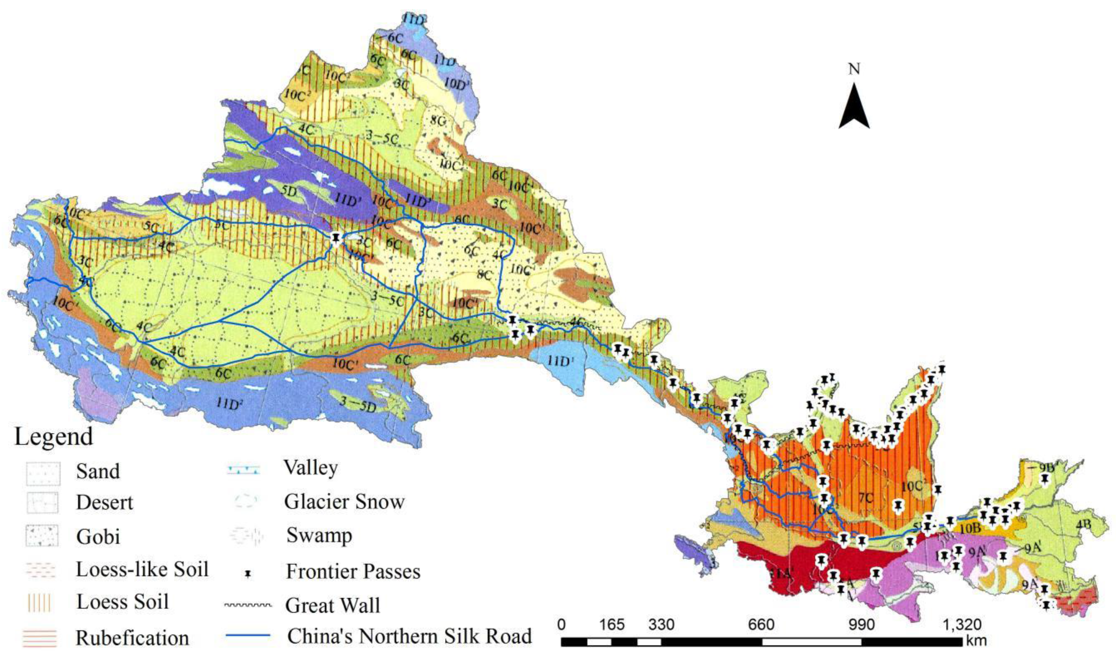
• The landform type and Average annual precipitation data set were applied to analyse the pattern of the frontier passes and provided by Data Centre for Resources and Environmental Sciences, Chinese Academy of Sciences (RESDC) [41].

2.2.2. Archaeological Data

The State Administration of Cultural Heritage (SACH) maintains an official record of the pass sites of the Ming Dynasty Great Wall based on the “Ming Dynasty Great Wall Investigation” undertaken by the National Administration of Surveying, Mapping, and Geoinformation [42]. We also used the Han Dynasty Great Wall collection by Luo [43], which is based on archeological materials, as a source. The frontier pass data were obtained through investigation and from existing research references [5,44]. In the study area, 86 recorded CNSR frontier passes, including the Great Wall gateways and main forts, were collected and used as sample data. In these passes, Yang pass has been destroyed and not preserved since the Tang Dynasty, so its location was set at Hongshan gateway according to existing research references. The other 85 passes are preserved today. All of the passes located in Xinjiang Uyghur Autonomous Region, Gansu Province, Ningxia Hui Autonomous Region, Shaanxi Province, and Henan Province are listed in

Table 1. List of 86 CNSR frontier pass sites.

Provinces and Autonomous Regions	Frontier Passes	Total Number
Xinjiang	Tiemen Pass	1
Gansu	Yumen Pass, Yang Pass, Jiayu Pass, Dazhen Pass, Liangzhou Wei, Suzhou Wei, Handong Wei, Yanzhi Fort, Suoqiao Fort, Lutang Fort, Tumen Fort, Dajing Cheng, Heishan Fort, Xiakou Fort, Shi Pass, Zhangye Cheng	16
Ningxia	Xiama Pass, Zhenyuan Pass, Sanguan Kou, Hengcheng Fort, Hengshan Fort, Xingwuying Suo, Guangwuying Suo, Qingshuiying Fort, Shengjin Pass, Daweikou Pass, Baisikou, Helankou, Yinchuan Cheng, Guyuan Cheng	14
Shaanxi	Dasan Pass, Jinsuo Pass, Tong Pass, Raofeng Pass, Wu Pass, Yangping Pass, Xiegu Pass, Yao Pass, Micang Pass, Xianren Pass, Longmen Pass, Wuli Pass, Luzi Pass, Linjin Pass, Yulin Cheng, Zhenbei Tower, Huangfuchuan Fort, Qingshuiying Fort, Gushan Fort, Zhenqiang Fort, Dabai Fort, Yongxing Fort, Gaojia Fort, Jian’an Fort, Changle Fort, Boluo Fort, Wuwei Fort, Huaiyuan Fort, Qingping Fort, Longzhou Fort, Zhenjing Fort, Zhenluo Fort, Jingbianying, Ningsai Fort, Liushujian Fort, Zhuanjing Fort, Dingbian Cheng	37
Henan	Changtai Pass, Wusheng Pass, Pingjing Pass, Jiuli Pass, Dasheng Pass, Yique Pass, Mengjin Pass, Heishi Pass, Dagu Pass, Hulao Pass, Jindi Pass, Xuanyuan Pass, Jingzi Pass, Luyang Pass, Qin Hangu Pass, Han Hangu pass, Zhuyang Pass, Liyang Pass	18

and labeled in Figure 1.

2.3. Method

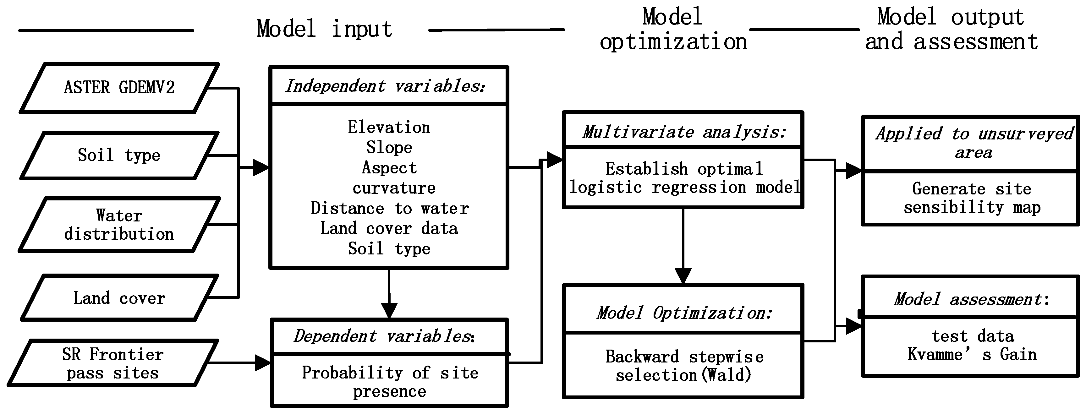
2.3.1. Binary Logistic Regression (BLR) Predictive Model

Due to the trade connection along the Silk Road, an associated and complex natural ecosystem was formed [45]. At a macro scale, the whole study area can be considered physiographically homogeneous, which is the underlying premise of the archaeological predictive model proposed by Kvamme [46].

There are three types of APMs model: deductive, inductive, and hybrid [47,48]. The prior-knowledge-based theoretical or deductive models that use intuition or deductive reasoning to model the relationships between archaeological sites and the landscape, such as the gravity model based on anthropological theory and the location-allocation (LA) model. The empirical or inductive models use statistical techniques to determine quantitative relationships between site locations and the environment, such as the multivariate statistical model with regression and decision functions. The decision tree model belongs to the theoretical and empirical hybrid model. APMs models were initially applied in archaeological settlement research to reveal correlations between circumstances and settlement locations. Since then, inductive models have been successfully applied in European, Asian, and American archaeology to reveal correlations between site distribution patterns and circumstances. The inductive model is a multivariate analysis method used to analyse the correlations between the independent and dependent variables and calculate the probability of an event occurrence. It avoids analysing the hypothesis and is feasible to analyse practical problems with natural proxies [49]. Kvamme’s research demonstrated that the BLR model is much more stable than other statistical methods used to create inductive predictive models [46]. Thus, in this study, the Binary Logistic Regression (BLR) model, as an inductive APM, is used.

In this research, the thematic data, which included elevation of ASTER GDEMV2, soil type, water distribution, and land cover of the frontier pass sites, were preprocessed as model input. Original independent variables were set based on these geospatial data, and the dependent variable was the occurrence probability of pass sites. Based on the multivariate analysis with logistic regression model and model optimization with Wald’s backward stepwise selection, a site sensibility map was generated after applying the model to the unsurveyed area. The test data and Kvamme’s Gain statistics were used to validate the model. The procedure is shown in Figure 2.

2.3.2. Model Variables

To obtain practical predictive results, the selection of independent variables takes the impact factors of site presence and distribution into account. The 17 independent variables shown in

Table 2. Independent variables for the Binary Logistic Regression (BLR) Archeological Predictive Models (APMs).

Independent Variable Name	Data Source	Type of Variable	Description
ELE	ASTER GDEMV2	Terrain (km)	Elevation
ASP			Aspect
SLO			Slope
CUR			Curvature
PLC			Plane curvature
PRC			Profile curvature
DS_IS	Diva GIS		Distance to intermittent streams
DS_PS			Distance to perennial streams
DS_4S	1:4,000,000 GIS data		Distance to Streams (4th orders and higher)
DS_5S	1:4,000,000 GIS data		Distance to Streams (5th orders and higher)
GL30(4)	GL30 land cover database		GL30 land cover
SOI_Typ(13)	Soil Classes HWSD v1.1	Non-terrain	Soil Type (FAO90)
IGB_LC(4)	IGBP-DIS land cover data		IGBP land cover
GLC2000_LC(4)	GLC2000 land cover data		GLC2000
UMD_LC(4)	UMd land cover data		UMd land cover
MOD_LC(4)	MODIS land cover data		MODIS land cover
WEST_LC(4)	WESTDC land cover data		WESTDC land cover

are selected based on prior theoretical research and archaeological field work [42]. Among these variables, the terrain variables include aspect, slope, curvature, plane curvature, and profile curvature. The relative datasets are calculated using the ASTER GDEMV2 elevation data. The non-terrain variables include distances to water, soil type, and land cover type. The distances to water are also analysed based on the terrain surface trends. The categorical variables, including the land cover and soils, were recoded and handled as dummy variables in the models. The class values of the land cover and soils were reclassified into 5 classes and 14 classes, respectively, considering the input data number and recoded into 4 binary dummy variables and 13 dummy variables, respectively, for the model. The soil class recoding was based on the soil order of FAO90. The land-cover class recoding index table is shown in

Table 3. Land-cover class recoding check list.

GLC2000_LC ID	New ID	GL30 ID	New ID	IGB_LC/MOD_LC ID	New ID	UMD_LC ID	New ID	WEST_LC ID	New ID
1	1	10–19	2	1	1	0	3	11	3
2	1	20–29	1	2	1	1	1	12	2
3	1	30–39	2	3	1	2	1	21	1
4	1	40–49	1	4	1	3	1	22	1
5	1	50–59	3	5	1	4	1	23	1
6	1	60–69	3	6	1	5	1	24	1
7	2	70–79	4	7	1	6	1	31	2
8	2	80–89	5	8	2	7	1	32	2
9	2	90–99	4	9	2	8	1	33	2
10	2	100	4	10	2	9	1	41	3
11	2	-	-	11	2	10	2	42	3
12	2	-	-	12	2	11	2	43	3
13	5	-	-	13	5	12	4	44	4
14	3	-	-	14	2	13	5	45	3
15	3	-	-	15	4	-	-	46	4
16	3	-	-	16	4	-	-	51	5
17	4	-	-	17	3	-	-	52	5
18	4	-	-	-	-	-	-	53	5
19	4	-	-	-	-	-	-	61	4
20	4	-	-	-	-	-	-	62	4
21	2	-	-	-	-	-	-	63	4
22	2	-	-	-	-	-	-	64	3
23	2	-	-	-	-	-	-	65	4
24	1	-	-	-	-	-	-	66	4
-	-	-	-	-	-	-	-	67	5

with the new recoded class ID 1 for forest and shrublands, 2 for grasslands and cultivated land, 3 for water bodies and wetland, 4 for glacier, bare rocks, and deserts, and 5 for city.

2.3.3. Model Optimization

In this study, the dependent variable for the BLR model is the site occurrence probability P (the range of P is [0, 1]), and 1 − P is the probability of site absence. The ratio of 1/(1 − P) is transformed by the logit transformation into ln (1/(1 − P)) and ranges from (−∞, +∞). The linear regression equation of logit P is

$$\ln (1/(1-P))={\alpha }_1{x}_1+{\alpha }_2{x}_2+\cdots +{\alpha }_n{x}_n+{\epsilon }_0={\displaystyle \sum _{\mathrm{i}=1}^{\mathrm{n}}{\alpha }_{\mathrm{i}}{x}_{\mathrm{i}}+}{\epsilon }_0$$

(1)

where, $x_{\mathrm{i}}$ is the independent variable, and ${\alpha }_i$ denotes the unknown regression coefficients to be calculated. However, APMs assume that the environmental factors that influence settlement choices are accurately represented in modern maps of environmental resources. The primary critique on the use of geographic data as predictor variables involves the reliability of available spatial datasets to accurately represent past environmental conditions. In fact, the reliability and accuracy of the final result depend on the spatial-temporal scale of the geospatial data. To express the impact on the predictive results of geospatial data, the spatial-temporal scale domain $D_{\mathrm{S}}$ should be imported into the model optimization

$$\ln (1/(1-P_S))={\displaystyle \sum _{\mathrm{i}=1}^{\mathrm{n}}{\alpha }_{\mathrm{i}}{}_S{x}_{\mathrm{iS}}+}{\epsilon }_{0S}(x_{iS}\in D_S).$$

(2)

Limited by the model input data timeliness, only the spatial scale is considered here. Because there is correlation among the terrain or non-terrain variables listed in Table 2, two scale domains $S_{terrain},S_{non-terrain}$ are set separately for the terrain variables and non-terrain variables, and Equation (3) is obtained as follows:

$$\ln (1/(1-P_s))={\displaystyle \sum _{\mathrm{i}=1}^{{\mathrm{n}}_{\mathrm{terrain}}}{\alpha }_{\mathrm{i}}{x}_{\mathrm{i}}+}{\displaystyle \sum _{\mathrm{j}=1}^{{\mathrm{n}}_{\mathrm{non}-\mathrm{terrain}}}{\beta }_{\mathrm{j}}{y}_{\mathrm{j}}+}{\epsilon }_0(x_i\in D_{terrain},y_i\in D_{non-terrain}).$$

(3)

Although $D_{terrain},D_{non-terrain}$ are continuous space domains, the domains were dispersed into 1000 m, 750 m, 500 m, 250 m, 100 m, and 50 m in practice. The input datasets for all of the variables were extracted at different scales for the site and non-site points to fit this improved BLR model. The backward stepwise selection method was used to screen the independent variables with different scales based on Wald’s test and Likelihood Ratio tests. All of the dummy variables were entered together, and the last variable was set as the reference class to compare the significant correlation between the other variables and site existing. The importance of each explanatory variable was assessed by the significance of the regression coefficients for different spatial scales. The error of the BLR model obeys a binomial distribution rather than a normal distribution.

The result of model optimization is given by

$$P=1/(1+e^{-({\displaystyle \sum _{i=1}^n{a}_i{x}_i+{\epsilon }_0})}).$$

(4)

A site sensibility map was generated in which each parcel in the study area was assigned a probability score. Each individual probability score was derived from the environmental characteristics of the parcel using Equation (4).

2.3.4. Model Assessment

Except for the test data validation, Kvamme’s Gain Statistics [50] is also a simple and practical method to verify the accuracy of a site prediction model:

$$KGain=1-P_{\mathrm{r}}/P_{\mathrm{t}}$$

(5)

where, in Equation (5), $P_{\mathrm{r}}$ and $P_{\mathrm{t}}$ are the area percentage and the number percentage for each probability level, respectively. A Kgain value close to 1 indicates that the model has strong predictive capability. In contrast, a Kgain value close to 0 indicates that the model has nearly no predictive ability. Finally, a Kgain value lower than 0 indicates that the model has reverse predictive ability: it can predict that a site does not exist.

3. Results

For the improved BLR predictive model, in the study area, 350 sample points, including 56 site and 294 confirmed non-site points used as training data, and 150 sample points, including 30 site points and 120 confirmed non-site points used as test data, were used to validate the model. Both the sample data and test data are distributed evenly. The model’s dependent variables are equal to 1 for site points and 0 for non-site points.

3.1. Model Optimization Result

There are only four recoded land-cover classes for site and non-site points and no points located in the city class; therefore, three dummy variables for GLC2000_LC were handled in the model. Through the significance tests, the variables shown in

Table 4. The statistical results of the predictive model for the CNSR frontier pass sites.

Independent Variables	B	Wald	Sig	Exp (B)
ELE	−1.055	12.574	0.001	0.348
SLO	−0.093	4.077	0.043	0.911
GLC2000_LC(1)	3.161	6.955	0.008	23.585
GLC2000_LC(2)	2.530	11.48	0.001	12.559
GLC2000_LC(3)	1.556	2.01	0.156	4.74
DS_PS	−0.045	6.989	0.008	0.956
Constant	5.4291	0.587	0.443	1.857

, ELE, SLO, and GLC2000_LC, including GLC2000_LC(1), GLC2000_LC(2), GLC2000_LC(3), and DS_PS, were reserved as the final inputs of the model. After backward stepwise variable selection, the best spatial scales are 50 m and 1000 m, respectively, for terrain and non-terrain variables. The input data of elevation, slope, land cover, recoded land cover, and distance to perennial streams are shown in Figure 3.

The statistical results of the model are listed in Table 4. B denotes the regression coefficients, Wald represents Wald’s ${\chi }^2$ statistics, Sig is the significance level, and Exp (B) is the odds ratio. The significance levels of all of the terrain variables, GLC2000_LC(1) and GLC2000_LC(2), are all below 0.05, which means they are correlated with the occurrence probabilities of CNSR frontier pass sites, while the significance level is a little higher than 0.1, that is, compared with GLC2000_LC(3), the vegetation classes are much more correlated with the site existing probabilities.

3.2. Site Sensibility Map

The site sensibility map was generated to label the probability of a pass existing. Jenks’ natural breaks were applied to classify the probability values into low (0–0.22), moderate (0.22–0.59), and high (0.59–0.90 and 0.90–1) grades. The higher the grade value, the higher the probability of pass site occurrence. Figure 4 shows the CNSR frontier pass site sensibility map with the grade values.

3.3. Model Assessment

A quantitative model assessment was conducted to validate the model using 350 input points and 150 test points. The resulting accuracy is shown in

Table 5. The prediction accuracy.

Data Types		Prediction Result		Precision/%	Overall Accuracy/%
		Non-Site	Site
Input data	Non-site (0)	254	40	86.4	86.7
	Site (1)	6	50	89.3
Test data	Non-site (0)	108	12	90.0	89.3
	Site (1)	4	26	86.7

.

Normally, a logical and repeatable inductive quantitative model should offer good performance in predicting archaeological site locations with accuracy in the range of 70–85% [51]. In this study, the overall prediction accuracy of the improved BLR model for the input data was 86.7%, in which site prediction precision was 89.3% and non-site prediction precision was 86.4% (the threshold was 0.5; when probability values are greater than 0.5, the points are considered to be sites, otherwise they are considered non-sites). For the test data, the total accuracy was 89.3% and the site prediction precision was 86.7%. The accuracy of the site predictive models is acceptable.

Kvamme’s gain values for each probability level in the reclassified sensibility map were also calculated and are shown in

Table 6. The Kvamme’s gain results for the site predictive model.

Probability Level	Area Percentage	Site Number	Number Percentage	Kgain
Low	52.78%	4	4.65%	−10.35
Moderate	25.20%	18	20.93%	−0.20
High	22.02%	64	74.42%	0.70

.

Table 6 shows that the high probability area accounts for 22.02% of the entire study area and 74.42% of sites with a Kvamme’s gain value of 0.70. This indicates that the model could effectively identify high-probability regions.

4. Discussion

4.1. Spatial-Temporal Scale and Model Reliability Analysis

It is shown that different variables had different scales for the scale optimization BLR model. For the terrain variables in this study, including ELE, SLO, CUR, PLC, PRC, DS_IS, DS_PS, and DS_4S, different spatial scales (1000 m, 750 m, 500 m, 250 m, 100 m, and the original 50 m) were used to fit the model. The regression coefficients and the accuracy of the final input independent variables after backward stepwise selection are listed in

Table 7. Regression coefficients and accuracy of different spatial scales.

Variables	1000 m	750 m	500 m	250 m	100 m	50 m
ELE	−1.444	−1.425	−1.397	−1.279	−1.092	−1.055
GLC2000_LC(1)	1.799	1.928	1.899	2.157	3.036	3.161
GLC2000_LC(2)	2.238	2.265	2.225	2.264	2.469	2.530
GLC2000_LC(3)	1.414	1.434	1.406	1.453	1.513	1.556
DS_PS	−0.041	−0.041	−0.042	−0.043	−0.045	−0.045
SLO	0.090	0.062	0.043	−0.007	−0.085	−0.093
Constant	0.475	0.464	0.500	0.483	0.661	0.619
Accuracy	86%	86%	86%	86.7%	86.7%	86.7%

and Figure 5.

From Table 7 and Figure 5, for terrain variables, the finer the resolution of the terrain data is, the higher the accuracy of the predictive model will be. The slope variable value changed from 0.090 to −0.093, because slope is more sensitive than other terrain factors to different spatial scales. Note that all of the accuracy values for all of the schemes are above 86% and the regression coefficients for the same terrain variables in the different schemes are similar, which means that the predictive model is relatively stable.

For non-terrain variables, such as land cover, smaller parcels better reflect the site distribution pattern of the study area at a macro scale. Land cover data with a parcel size of 1000 m were finally reserved on the basis of variable selection compared with land cover data with larger parcel sizes. Experiments demonstrated that land cover data with an original parcel size of 1000 m do not provide the same results as land cover data resampled from a higher resolution. The 1000 m land cover data obtained from low-resolution remote sensing image interpretation is much more useful for CNSR pass site prediction. Furthermore, using the best land cover scale of 1000 m and a terrain scale of 50 m, different land cover data were also compared. The result showed that the accuracies of IGBP, MODIS, UMd, and WESTDC land cover data with parcel sizes of 1000 m all reached 84%, only slightly lower than that reached using the GLC2000 data. This demonstrates that all land cover data with a parcel size of 1000 m can be used to construct predictive models of CNSR frontier pass sites.

For non-terrain variables, such as water distribution, five combination schemes with different spatial scales were tested. The accuracy values from these different schemes are listed in

Table 8. Accuracy of five water variable combination schemes at different scales.

	Input Water Variables	1000 m	750 m	500 m	250 m	100 m	50 m
accuracy	Distance to perennial streams, distance to intermittent streams, distance to streams (4th order and higher) and distance to streams (5th order and higher)	86%	86%	86%	86.7%	86.7%	86.7%
	Distance to all the streams merging perennial streams and intermittent streams	72.7%	78.7%	76.7%	74.7%	74.7%	75.3%
	Distance to perennial streams, distance to intermittent streams	82%	82%	82%	81.3%	81.3%	81.3%
	Distance to streams (4th order and higher) and streams (5th order and higher)	80.7%	82%	83.3%	80%	76%	82%
	Distances to streams (5th order and higher)	81.3%	79.3%	80%	80%	76%	81.3%

. All of the listed combinations of distances to streams were provided as input to the model, while the distance to perennial streams or streams (4th order and higher) was reserved as the final input variable. When the distance to all streams (merging perennial streams and intermittent streams) are input to the model as the only water input variable, the accuracy decreases by between 9.23% and 16.15%. Perennial streams or headwaters change much more slowly than intermittent streams. As a result, the perennial streams or headwaters from modern maps can be used to predict frontier pass site locations. This result also demonstrates that perennial streams or headwaters have a stronger impact on site location than do intermittent streams or all streams, which supports the theory that the ancient CNSR frontier passes were built while considering the long-term water supply available for both caravans and troops by channelling water from non-seasonal streams.

From the result, it is also demonstrated that terrain variables are relatively stable through time, that is, terrain changed not a lot and is similar to that in a paleo-environment. Land cover and hydrology variables vary over time and are influenced by paleo-climate and paleo-environment. For land cover and water distribution, the essential question is: How relevant are the ‘distance to water’ and land cover variables if the course of rivers or the type of land cover has changed over time? From previous cases in which predictive models were successfully applied, there are two supporting concepts for these questions: choosing areas with slow temporal changes and proper spatial scales for the environmental conditions [11,52].

4.2. Contribution Factor Analysis

From the final predictive model, the spatial distribution of the CNSR frontier passes is correlated with elevation, slope, land cover, and distance to perennial streams data. The independent variable statistical results are shown in Figure 6. The curve of the reserved input variables is fixed by a moving average of the site frequencies taken two bins at a time.

From Figure 6, the predictive model of CNSR frontier pass sites is remarkably well-correlated with the terrain. The average elevation and the slope are 1389.96 m and 5.96° for the site points, respectively, while they are 2484.97 m and 10.16° for the non-site points, respectively. All of the frontier pass sites were also added on the climate landform type map in Figure 7 and the climate landform types for Figure 7 are listed in

Table 9. The climate landform type list of Figure 7.

Basic Types	Climate Landform Type	A Humid Monsoon Climate Landform	B Warm Humid and Semi-Humid Monsoon Climate Landform	C Inland Arid and Semi-Arid Climate Landform	D Alpine Cold–High Latitude Climate Landform
Plain	1 River delta			-	-
	2 Marine plain	deposition	deposition	-	-
		abrasion	abrasion
	3 Alluvial-Lacustrine plain			Salt lake plain, playa lake plain	Freeze–thaw plain
	4 Alluvia plain
	5 Alluvium-diluvium wave plain
	6 Alluvial sloping plain	-	-		Earthflow platform
Platform and Highland	7 Platform and Terrace
	8 Piedmont plain and Highland	Low	Low	Highland	Highland
		High	High
Hill and Mountain	9 Hill	Erosion	Erosion	Arid denudation	Frosting wind-erosion
		Corrosion	Corrosion	Erosion and Denudation	Frosting erosion
	10 Low mountain and Middle mountain	Erosion	Erosion	Arid denudation	Frosting
					Frosting wind-erosion
		Corrosion	Corrosion	Erosion and Denudation	Frosting erosion
	11 High mountain and Extra-high mountain	Erosion	-	-	Frosting
					Frosting wind-erosion
		Valley			Frosting erosion

. Over 60% of the site points are located at altitudes between 1000 m and 1700 m, with gentle slopes below 6°. Most of the passes are located near the water sources, especially in the Guannei part from the local window of Figure 4. The western frontier pass sites near the historical national borders are located in the area of the arid and semi-arid climate landform labelled with 6C, 9C, and 10C. The frontier pass sites in the eastern part with the monsoon climate landform are mainly located in the hills and mountains labelled with 9A, 10A, and 11A. Most of the frontier pass sites are located among different landforms and under erosion circumstances. That is because the frontier passes are always distributed in “easy to defend and hard to attack” regions, such as mountainous valleys near water, or in the Gobi where it is easier to control the main routes and build city walls.

Furthermore, the areas with high probability are all located near perennial streams. Although intermittent streams are important for the desert-oasis routes—especially in the western sections—perennial streams and headwaters are still the main water sources for the CNSR frontier pass sites. As an important defense system in ancient China, the frontier passes tended to be located at regions with adequate long-term water supplies; consequently, as the distance from perennial streams increases, the occurrence probability of pass sites decreases, which agrees with our knowledge. From the model, the distances to perennial streams were selected as independent variables rather than the distances to intermittent streams or to all streams. The average distance to perennial streams for pass sites is 6.13 km, whereas for non-sites that distance is 33.94 km. Some 78.57% and 62.5% of sites are respectively located within 10 km of perennial streams. In addition, the final predictive model was negatively correlated with the land-cover class recoded value from GLC2000. From the statistical results, the main land-cover classes for sites are grassland, cultivated land, and forest or shrublands, while gravel and desert are the main classes for non-site data, especially in the western part of the study area. In other words, most of the confirmed CNSR frontier pass sites are mainly distributed in natural surface regions that are covered by vegetation today.

4.3. Pattern Analysis of CNSR Frontier Pass Distribution

The theoretical basis of predictive modelling depends on two factors: non-random human behaviour and environmental factors. The spatial patterns of archaeological sites can be used to explore the relationships between ancient human activity locations and the distribution of certain environmental resources [53,54,55].

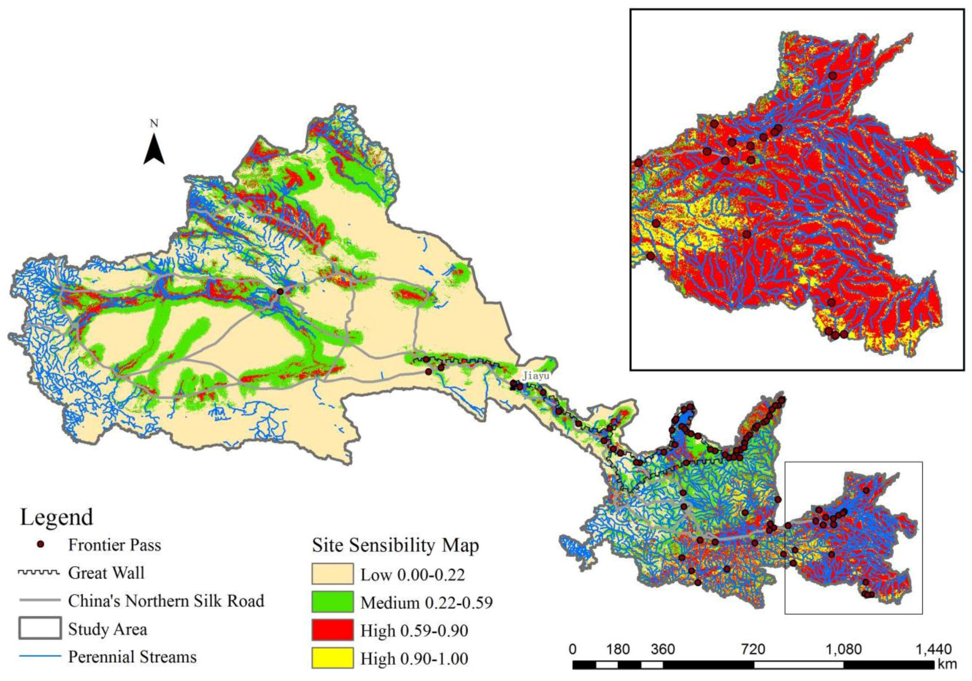
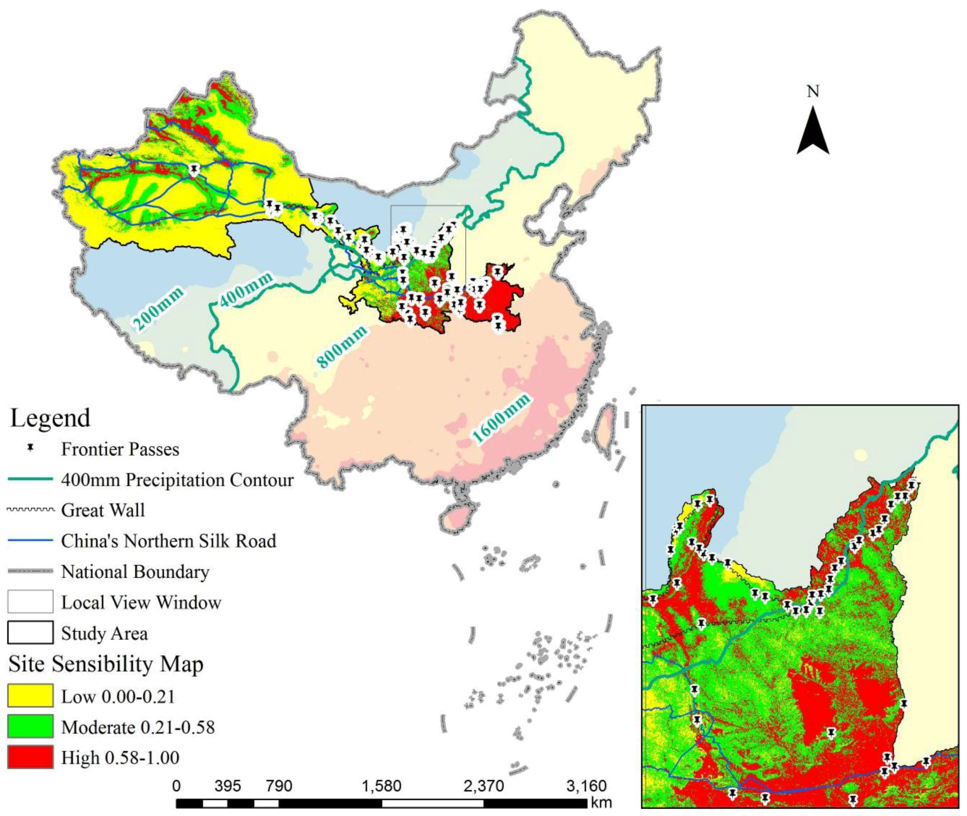
• According to the site sensibility map in Figure 4, the distribution of CNSR frontier passes has clustering characteristics: the high site probability region is mainly located in the east and north, and the low probability region is mainly in the west or south with the division overlapped with the average annual precipitation of 400 mm. These characteristics are consistent with the pass site distribution; eastern is dense and western is rare. The pass-dense region is also called “Guanzhong” or “Guannei” and belonged to the territory controlled by most ancient Chinese dynasties. Otherwise, it is interesting to note that the Great Wall frontier pass line nearly overlaps the division of precipitation of 400 mm in Shaanxi province as shown in the local view window of Figure 8. This may be because these Great Wall frontier passes were fortifications that protected the more livable central plains from the nomadic tribes, particularly from attacks by the Huns.
• Although passes are rare in the western part, only one site in Xinjiang Uyghur Autonomous Region and four sites west of Jiayu Pass, and in the vicinity of the Great Wall or the Silk Road, were not used as model inputs either. The areas with high and moderate probability in the sensibility map are spatially overlapped with the Han Great Wall section (from Yumen pass to Jiayu pass) and with three western parts of the CNSR routes, as shown in Figure 4. This result demonstrated that the improved BLR model was able to reveal the spatial correlation characteristics of frontier passes and the Great Wall, and could be used to reconstruct ancient trade routes.

5. Conclusions

Reconstructing and investigating the Silk Road historical environment is a great challenge, and it requires systematic research at both spatial and temporal scales [56]. Understanding the relationships among the punctate distribution of frontier pass sites, the linear distribution of the Great Wall and Silk Road routes, and the zonal distribution of the Silk Road Economic Belt is helpful in fully understanding the Silk Road ecosystem and for the protection of these historical remains. In this study:

• APMs can be used as a pattern tool for macro-scale site distribution and a temporal-spatial scale can be imported into the APMs [57,58]. An improved BLR model with spatial-scale optimization was successfully constructed and validated to analyze the spatial distribution of CNSR frontier passes in this study. The high probability areas identified through the study were helpful for further archaeological interpretation and archaeological validation.
• Through spatial-temporal analysis, the best spatial scale should be considered and the best parcel size selection varies with the stability of the variables. Selecting resources that change slowly, such as perennial streams connected with site locations, is helpful in reconstructing ancient environments using modern data. The best scale spatial for the terrain variables and the non-terrain variables are 50 m and 1000 m, respectively.
• Based on the variable selection, the elevation, slope, land cover, and distances to perennial streams were identified as the independent variables used to construct the model. An assessment of the model from the sample data and Kvamme’s gain statistics verified that the predictive model can effectively identify regions with a high probability of pass site occurrences, and it is able to reveal correlations between the pass sites and natural proxies.
• The distribution of CNSR frontier passes has clustering characteristics; the high probability area was mainly located in the east, and the division between the low and moderate-to-high areas coincides with the 400 mm precipitation contour. In the site sensibility map, the high and medium probability areas cover the Great Wall and the CNSR routes, especially the western parts. The predictive model for archaeological sites was shown to be helpful for analysing the spatial distribution pattern of CNSR pass sites used for both military defense systems and as trade control stations.

References

1. Zhao, C.; Zhang, C. Military Remains of the Silk Road from the Perspective of Archaeology. Cult. Relics 2016, 2, 73–80. (In Chinese) [Google Scholar] [CrossRef]
2. Von Richthofen, F. China, Ergebnisse Eigner Reisen und Darauf Gegründeter Studien (China: The Results of My Travels and the Studies Based Thereon), 1st ed.; Dietrich Reimer: Berlin, German, 1877. [Google Scholar]
3. Daniel, C.W. Richthofen’s “Silk Roads”: Toward the Archaeology of a Concept. Silk Road 2007, 5, 1–10. [Google Scholar]
4. Elisseeff, V. The Silk Roads: Highways of Culture and Commerce; UNESCO Publishing/Berghahn Books: New York, NY, USA, 2001. [Google Scholar]
5. Li, S.; Liang, R. The Great Wall-Shaanxi, Ningxia, Gansu; China Travel & Tourism Press: Beijing, China, 2008. (In Chinese) [Google Scholar]
6. UNESCO World Heritage Sites. “The Great Wall”. Available online: http://whc.unesco.org/en/list/438/ (accessed on 20 December 2017).
7. UNESCO World Heritage Sites. “Silk Roads: The Routes Network of Chang’an-Tianshan Corridor”. Available online: http://whc.unesco.org/en/list/1442/ (accessed on 20 December 2017).
8. Zhang, M. On the Territory of the Ancient Silk Road Pingchuan District Ferry and the Ruins of the Ancient City. Silk Road 2015, 291, 27–29. [Google Scholar]
9. Chen, F.; Masini, N.; Liu, J.; You, J.; Lasaponara, R. Multi-Frequency Satellite Radar Imaging of Cultural Heritage: The Case Studies of the Yumen Frontier Pass and Niya Ruins in the Western Regions of the Silk Road Corridor. Int. J. Digit. Earth 2016, 9, 1224–1241. [Google Scholar] [CrossRef]
10. Chen, F.; Lasaponara, R.; Masini, N. An overview of Satellite Synthetic Aperture Radar Remote Sensing Inarchaeology: From Site Detection to Monitoring. J. Cult. Herit. 2015, 23, 5–11. [Google Scholar] [CrossRef]
11. Luo, L.; Wang, X.; Liu, C.; Guo, H.; Du, X. Integrated RS, GIS and GPS Approaches To Archaeological Prospecting in the Hexi Corridor, NW China: A Case Study of the Royal Road to Ancient Dunhuang. J. Archaeol. Sci. 2014, 50, 178–190. [Google Scholar] [CrossRef]
12. Verhagen, P.; Whitley, T.G. Integrating Archaeological Theory and Predictive Modeling: A Live Report From the Scene. J. Archaeol. Method Theory 2012, 19, 49–100. [Google Scholar] [CrossRef]
13. Gao, L. Space-Time Explanation New Method-History, Present and Future of GIS Research in European and American Archaeology. Archaeology 1997, 89–95. [Google Scholar]
14. Whitley, T.G. Archaeological Simulation and the Testing Paradigm. In Uncertainty and Sensitivity Analysis in Archaeological Computational Modeling; Springer: Berlin, Germany, 2016; pp. 131–156. [Google Scholar]
15. Mei, Q.; Xiong, X. Application of GIS in Archaeology. J. Zhejiang Wanli Univ. 2005, 18, 32–35. (In Chinese) [Google Scholar]
16. Mcewan, D.G. Qualitative Landscape Theories and Archaeological Predictive Modelling—A Journey Through no Man’s Land? J. Archaeol. Method Theory 2012, 19, 526–547. [Google Scholar] [CrossRef]
17. Bevan, A.; Wilson, A. Models of Settlement Hierarchy Based on Partial Evidence. J. Archaeol. Sci. 2013, 40, 2415–2427. [Google Scholar] [CrossRef]
18. Danese, M.; Masini, N.; Biscione, M.; Lasaponara, R. Predictive Modeling for Preventive Archaeology: Overview and Case Study. Open Geosci. 2014, 6, 42–55. [Google Scholar] [CrossRef]
19. Willey, G.R. Prehistoric Settlement Patterns in the Virú Valley, Peru; Bureau of American Ethnology, Bulletin: Washington, DC, USA, 1953.
20. Vaughn, S.; Crawford, T. A Predictive Model of Archaeological Potential: An Example from Northwestern Belize. Appl. Geogr. 2009, 29, 542–555. [Google Scholar] [CrossRef]
21. Carrer, F. An Ethnoarchaeological Inductive Model for Predicting Archaeological Site Location:A Case-Study of Pastoral Settlement Patterns in the Val di Fiemmeand Val di Sole (Trentino, Italian Alps). J. Anthropol. Archaeol. 2013, 32, 54–62. [Google Scholar] [CrossRef]
22. Balla, A.; Pavlogeorgatos, G.; Tsiafakis, D.; Pavlidis, G. Locating Macedonian Tombs Using Predictive Modelling. J. Cult. Herit. 2013, 14, 403–410. [Google Scholar] [CrossRef]
23. Oonk, S.; Spijker, J. A Supervised Machine-Learning Approach towards Geochemical Predictive Modelling in Archaeology. J. Archaeol. Sci. 2015, 59, 1–9. [Google Scholar] [CrossRef]
24. Sharafi, S.; Fouladvand, S.; Simpson, I.; Alvarez, J. Application of pattern recognition in detection of buried archaeological sites based on analysing environmental variables, Khorramabad Plain, West Iran. J. Archaeol. Sci. Rep. 2016, 8, 206–215. [Google Scholar] [CrossRef]
25. Vogel, S.; Märker, M.; Esposito, D.; Seiler, F. The Ancient Rural Settlement Structure in the Hinterland of Pompeii Inferred From Spatial Analysis and Predictive Modeling of Villae Rusticae. Geoarchaeology 2016, 31, 121–139. [Google Scholar] [CrossRef]
26. Negre, J.; Munoz, F.; Lancelotti, C. Geostatistical Modelling of Chemical Residues on Archaeological Floors in the Presence of Barriers. J. Archaeol. Sci. 2016, 70, 91–101. [Google Scholar] [CrossRef]
27. Ni, J. Predictive Model of Archaeological Sites in the Upper Reaches of the Shuhe River in Shandong. Process Geogr. 2009, 28, 489–493. (In Chinese) [Google Scholar]
28. Peng, S.; Zhang, W.; Chen, D. Model Predictability of Archaeological Sites of the Dawenkou Culture in the Wensi River Basin. J. Taishan Univ. 2010, 32, 34–39. (In Chinese) [Google Scholar]
29. Qiao, W.; Bi, S.; Wang, Q.; Guo, Y. Predictive model of archaeological sites of Longshan culture in Zhengzhou-Luoyang area. Sci. Surv. Mappin 2013, 38, 172–174, 181. (In Chinese) [Google Scholar]
30. Dong, Z.; Jin, S. Prediction Research on Bohai Kingdom Ruins in Yanbian Area Based on the Logic Regression Model. J. Yanbian Univ. (Nat. Sci.) 2015, 41, 179–184. (In Chinese) [Google Scholar] [CrossRef]
31. Tianditu Website. Available online: http://en.tianditu.com/ (accessed on 20 January 2018).
32. Loveland, T.R.; Reed, B.C.; Brown, J.F.; Ohlen, D.O.; Zhu, Z.; Yang, L.; Merchant, J.W. Development of a Global Land Cover Characteristics Database and IGBP DISCover From 1 km AVHRR Data. Int. J. Remote Sens. 2000, 21, 1303–1330. [Google Scholar] [CrossRef]
33. Bartholomé, E.; Belward, A.S. GLC2000: A New Approach to Global Land Cover Mapping From Earth Observation Data. Int. J. Remote Sens. 2005, 26, 1959–1977. [Google Scholar] [CrossRef]
34. Hansen, M.C.; Defries, R.S.; Townshend, J.R.G.; Sohlberg, R. Global Land Cover Classification at 1 km Spatial Resolution Using a Classification Tree Approach. Int. J. Remote Sens. 2000, 21, 1331–1364. [Google Scholar] [CrossRef]
35. Friedl, M.A.; Mciver, D.K.; Hodges, J.C.F.; Zhang, X.Y.; Muchoney, D.; Strahler, A.H.; Woodcock, C.E.; Gopal, S.; Schneider, A.; Cooper, A.; et al. Global Land Cover Mapping From MODIS: Algorithms and Early Results. Remote Sens. Environ. 2002, 83, 287–302. [Google Scholar] [CrossRef]
36. Usman, M.; Liedl, R.; Shahid, M.A.; Abbas, A. Land Use/Land Cover Classification and its Change Detection Using Multi-Temporal MODIS NDVI Data. J. Geogr. Sci. 2015, 25, 1479–1506. [Google Scholar] [CrossRef]
37. Cold and Arid Regions Sciences Data Center Website. “Land Cover Products of China”. Available online: http://westdc.westgis.ac.cn (accessed on 20 December 2017).
38. Tianditu Website. Available online: http://zhfw.tianditu.com/ (accessed on 20 December 2017).
39. Free Spatial Data-DIVA GIS Website. Available online: www.diva-gis.org/Data/ (accessed on 20 December 2017).
40. ASTER GDEMV2 Download Website. Available online: http://gdem.ersdac.jspacesystems.or.jp/ (accessed on 20 December 2015).
41. Website of Data Center for Resources and Environmental Sciences, Chinese Academy of Sciences (RESDC). Available online: http://www.resdc.cn (accessed on 20 December 2017).
42. Chen, J.; Jin, S.; Liao, A.; Zhao, Y.; Xu, L.; Rong, D.; Yang, Z. An Overview of Investigation and Measurement of Ming Great Wall Resources. Geomat. World 2011, 11–16. (In Chinese) [Google Scholar]
43. Luo, L. Space Archaeology for Tunshu Sites along the South Route of the Ancient Silk Road. Ph.D. Thesis, the University of Chinese Academy of Sciences, Beijing, China, 2016. (In Chinese). [Google Scholar]
44. Cao, Y. Chinese Famous Frontier Passes; The People’s Liberation Army Press: Beijing, China, 1988. (In Chinese) [Google Scholar]
45. Shan, Q. On Lineal or Serial Cultural Heritages Protection Breakthrough and Pressure. Relics from South 2006. [Google Scholar] [CrossRef]
46. Kvamme, K.L. The Fundamental Principles and Practice of Predictive Archaeological Model. Math. Inf. Sci. Archaeol. A Flex. Framew. 1990, 3, 257–295. [Google Scholar]
47. Zhang, H. GIS and Archaeology Spatial Analysis; Beijing University Press: Beijing, China, 2014. [Google Scholar]
48. Conolly, J.; Lake, M. Geographical Information Systems in Archaeology; Cambridge University Press: Cambridge, UK, 2006. [Google Scholar]
49. Liang, Q.; Meng, W.; Lin, L.; Wan, Q. Potential Lightning Predictive Method Based on Logistic Regression Model. Guangdong Meteorol. 2011, 33, 44–51. (In Chinese) [Google Scholar] [CrossRef]
50. Kvamme, K.L. Computer Processing Techniques for Regional Modeling of Archaeological Site Locations. Adv. Comp. Archaeol. 1983, 1, 26–52. [Google Scholar]
51. Kvamme, K.L. There and Back Again: Revisiting Archaeological Locational Modelling. GIS and Archaeological Site Location Modelling; CRC Press Taylor & Francis Group: Boca, Raton, FL, USA, 2006. [Google Scholar] [CrossRef]
52. Yang, Y.; Zhang, S.; Yang, J.; Chang, L.; Bu, K.; Xing, X. A Review of Historical Reconstruction Methods of land Use/Land Cover. J. Geogr. Sci. 2014, 24, 746–766. [Google Scholar] [CrossRef]
53. Guo, Y.; Mo, D.; Mao, L.; Wang, S.; Li, S. Settlement Distribution and its Relationship with Environmental Changes from the Neolithic to Shang-Zhou Dynasties in Northern Shandong, China. J. Geogr. Sci. 2013, 23, 679–694. [Google Scholar] [CrossRef]
54. Li, K.; Zhu, C.; Jiang, F.; Li, B.; Wang, X.; Cao, B.; Zhao, X. Archaeological Sites Distribution and its Physical Environmental Settings between ca 260–2.2 ka BP in Guizhou, Southwest China. J. Geogr. Sci. 2014, 24, 526–538. [Google Scholar] [CrossRef]
55. Carlson, R.J.; Baichtal, J. A Predictive Model for Locating Early Holocene Archaeological Sites Based on Raised Shell-Bearing Strata in Southeast Alaska, USA. Geoarchaeology 2016, 30, 120–138. [Google Scholar] [CrossRef]
56. Li, M. Review on the 100 years’ Studies of the Silk Road. N. W. Ethno-Natl. Stud. 2005, 45, 48–49. [Google Scholar] [CrossRef]
57. Wang, J.; Deng, M.; Cheng, T.; Huang, J. Time-Spatial Data Analysis and Model; Sicence Press: Beijing, China, 2012. (In Chinese) [Google Scholar]
58. Demján, P.; Dreslerová, D. Modelling Distribution of Archaeological Settlement Evidence Based on Heterogeneous Spatial and Temporal Data. J. Archaeol. Sci. 2016, 69, 100–109. [Google Scholar] [CrossRef]
Figure 1. Geographic extent of the study area of China’s Northern Silk Road (CNSR) region (The Inset map is the ancient Silk Road route from Tianditu [31]).
Heritage 01 00002 g001
Figure 2. The procedure of predictive models of frontier pass site. SR: Silk Road.
Heritage 01 00002 g002
Figure 3. Model input data: (a) elevation, (b) slope, (c) land cover, (d) recoded land cover, and (e) distance to perennial streams.
Heritage 01 00002 g003aHeritage 01 00002 g003b
Figure 4. Sensibility map of the CNSR frontier pass sites.
Heritage 01 00002 g004
Figure 5. Regression coefficients and accuracy of different spatial scales.
Heritage 01 00002 g005
Figure 6. Independent variable statistical results: (a) elevation, (b) slope, (c) land cover, and (d) distance to perennial streams.
Heritage 01 00002 g006aHeritage 01 00002 g006b
Figure 7. The distribution of 86 frontier pass sites on the climate landform type map.
Heritage 01 00002 g007
Figure 8. Division of low and moderate-to-high probability CNSR frontier pass areas compared with the average annual precipitation line and the Great Wall.
Heritage 01 00002 g008