Propagating Dam Breach Parametric Uncertainty in a River Reach Using the HEC-RAS Software


1
Laboratory of Reclamation Works and Water Resources Management, School of Rural and Surveying Engineering, National Technical University of Athens, 15780 Athens, Greece
2
SEEMAN ENVIRONMENTAL, 14576 Athens, Greece
*
Author to whom correspondence should be addressed.
Hydrology 2020, 7(4), 72; https://0-doi-org.brum.beds.ac.uk/10.3390/hydrology7040072
Submission received: 6 September 2020
/
Revised: 30 September 2020
/
Accepted: 1 October 2020
/
Published: 3 October 2020
(This article belongs to the Special Issue Advances and Perspectives in Flood Risk Modeling, Assessment and Communication)
Abstract
:Dam break studies consist of two submodels: (a) the dam breach submodel which derives the flood hydrograph and (b) the hydrodynamic submodel which, using the flood hydrograph, derives the flood peaks and maximum water depths in the downstream reaches of the river. In this paper, a thorough investigation of the uncertainty observed in the output of the hydrodynamic model, due to the seven dam breach parameters, is performed in a real-world case study (Papadiana Dam, located at Tavronitis River in Crete, Greece). Three levels of uncertainty are examined (flow peak of the flood hydrograph at the dam location, flow peaks and maximum water depths downstream along the river) with two methods: (a) a Morris-based sensitivity analysis for investigating the influence of each parameter on the final results; (b) a Monte Carlo-based forward uncertainty analysis for defining the distribution of uncertainty band and its statistical characteristics. Among others, it is found that uncertainty of the flow peaks is greater than the uncertainty of the maximum water depths, whereas there is a decreasing trend of uncertainty as we move downstream along the river.
1. Introduction
Floods created by the failure of human structures, such as dams or levees, are included among the most significant hazardous events, mainly due to the very significant impact at the inundated area and the small predictability of the event. Usually, such types of events create huge and abrupt flood waves with destructive consequences, whilst the failure cause is not always related to the bad meteorological conditions, as usually observed during flood events. For example, the flood wave which hit Vajont was created by a landslide which fell into the Vajont dam reservoir [1], Malpasset and Teton dam breaches were created due to geological problems combined with structural failures [2,3]. One of the most destructive events, which occurred in 1938, was the Yellow River flood (the fatalities were about 900,000 whilst 4,000,000 people were displaced during the decade 1938–1947), which was created by sabotage during the second Sino-Japanese war [4]. An indicative list of dam breaks over the 20th century can be found at [5].
Due to the significant consequences accounted after a hypothetical dam failure, it is wise to deliver a dam break study, before its construction. It is noted that large numbers of dams of hydroelectric power production are currently planned or under construction in many areas around the world [6]. This study can be divided into two steps: (a) the breach modeling, in which the failure mechanism is simulated and the output is the flood hydrograph created by the breach formation; (b) the hydrodynamic modeling, in which the flood hydrograph is simulated as propagating to the area downstream of the dam. The output in this case is the maximum of discharge and the water stage at the inundated area. In other words, these two steps can be considered as two submodels which are linked using the Integrated Catchment Modeling framework, in which every process included in the water cycle is approached with a submodel, whilst the final output is derived through the linkage of the submodels used [7].
For the dam breach modeling, several parameters are required, which can be divided into the following groups: (a) geometrical characteristics of the breach (e.g., width of the breach, slopes of the breach, etc.); (b) required time for the formation of the breach; (c) flow characteristics of the breach (flow coefficient over the breach, similar to a weir coefficient, initial water stage at the reservoir). The parametric estimation depends on the type of the dam (e.g., earthfill vs. concrete dams) and the failure mechanism (e.g., overtopping vs. internal erosion) and can be performed either by selecting values from handbooks and regulations (in the cases that exist) or using statistical-based empirical models, such as developed by [8,9,10,11,12].
The flood hydrograph, which is the output of the breach modeling phase, is one of the inputs for the hydrodynamic submodels that are mainly based on either one-dimensional (1D) or two-dimensional (2D) forms of Shallow Water Equations (SWE). The other input is the geometry of the river located downstream of the dam. The parameters required for these types of models can be divided into the following categories: (a) parameters related to the boundary conditions (upstream, downstream, and internal); (b) friction coefficients of the computational domain (e.g., Manning coefficients); (c) parameters related to the numerical method used to solve the SWE (e.g., space step, time step, etc.). Several works for propagating the flood wave created by a dam failure can be found in the related literature [1,13,14,15,16,17], whilst several researchers tried to reconstruct a posteriori, collecting data from the field using various methods [18].
In our era, there are several commercial integrated platforms which link the submodels required for a proper dam break study, namely the dam breach and the hydrodynamic submodels. A special mention shall be made to the pioneer in that scientific area, which is the FLDWAV software (former DWOPER and DAMBRK codes), developed by the National Weather Service (NWS) of USA [19]. Other options for dam break studies are the open-source IBER software [20] and the well-known HEC-RAS software [21], used in this paper and also by many other researchers [22,23,24].
Both submodels are characterized by uncertainties, which have been observed [25,26,27]. The limitations for estimating the potential damages created by a dam failure due to uncertainty aspects are also reported by [28]. In this study, we perform a thorough investigation of the uncertainty observed in the output of the hydrodynamic submodel, due to the parametric uncertainty of the dam breach submodel, which is also input data uncertainty for the hydrodynamic submodel. For the investigation, a real-world case study is selected, and specifically for a Roller Compacted Concrete (RCC) dam.
As far as the static behavior is concerned, RCC dams are a hybrid version of earthfill and concrete dams. Compared to the conventional types of dams, RCC material has recently started to be used. The main reasons for selecting this type of dam are the following: (a) although the RCC dams are less vulnerable to failure in comparison with earthfill dams, many countries have adopted a relative legislation which enforces the implementation of dam break studies; (b) in our era, since RCC dams are relatively cheap and couple the advantages of earthfill and concrete dams, they are widely used; (c) the recent nature of this type of dam has the consequence that many topics are uninvestigated, one of which is the dam breach mechanism. Therefore, bigger uncertainty issues exist in a potential dam failure, compared with the conventional type of dams.
First, we implement a Morris method-based sensitivity analysis, for quantifying the influence of each parameter on the output. Second, we implement a Monte Carlo-based uncertainty analysis for estimating the uncertainty band of the output, selecting a proper distribution and finding its statistical characteristics. Both sensitivity and uncertainty analyses are performed in the spatial scale, namely along the river located downstream of the dam.
Finally, it is noted that for this study, only the parameters of the breach submodel are under examination and not the parameters of the hydrodynamic submodel. Although parametric uncertainty of hydrodynamic models can be significant [29], in this work we decided to investigate only the parametric uncertainty of the dam breach submodel, due to the chaotic nature of the dam failure, which is difficult to be defined either by a deterministic or by a probabilistic procedure (e.g., we cannot determine the return period of the failure).
2. Materials and Methods
2.1. Case Study
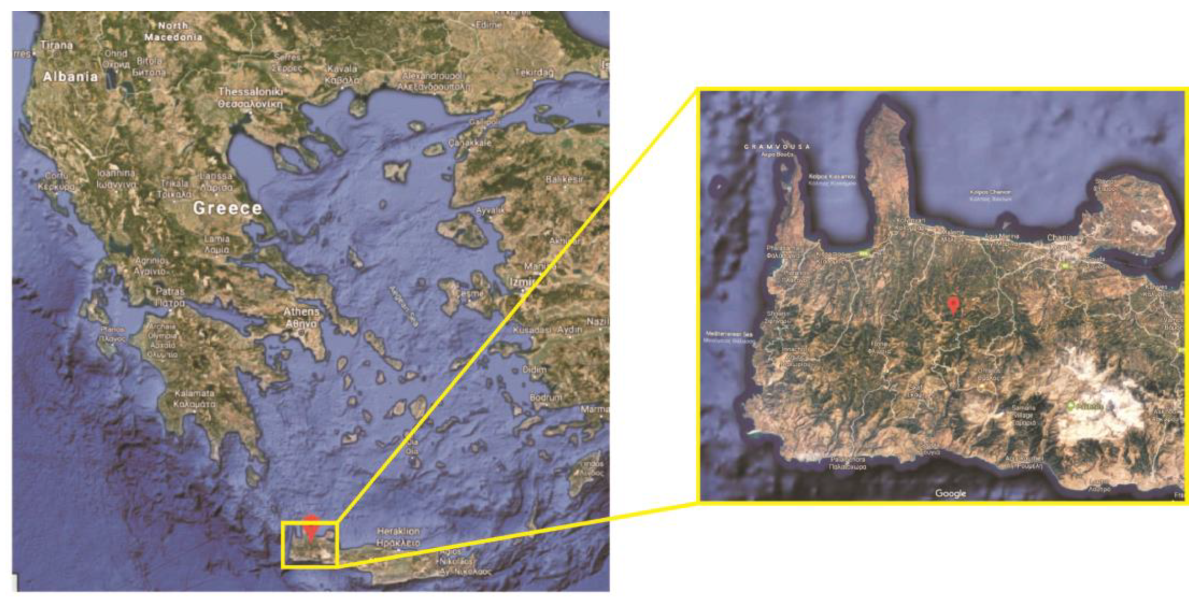
The selected case study is the Papadiana Dam (which is at the final design stage), located at the Tavronitis River in the island of Crete, Greece. The type of the dam is an RCC dam, which will create a reservoir of 25 × 106 m3. The crest length is 330 m. The elevation of the river bottom is expected to be at +237 m AMSL(Above Mean Sea Level), the maximum normal level of the dam (spillway level) is defined to be at +326 m AMSL, and the crest level is designed to be at +329 m AMSL. Considering that foundation depth is 10 m, the total height of the dam is 102 m, whilst the net height (from river bottom to the crest) is 92 m. The Tavronitis River has a length of about 15 km from the dam location to the estuary at the sea. Figure 1 depicts the location of the dam.
2.2. Breach Modeling
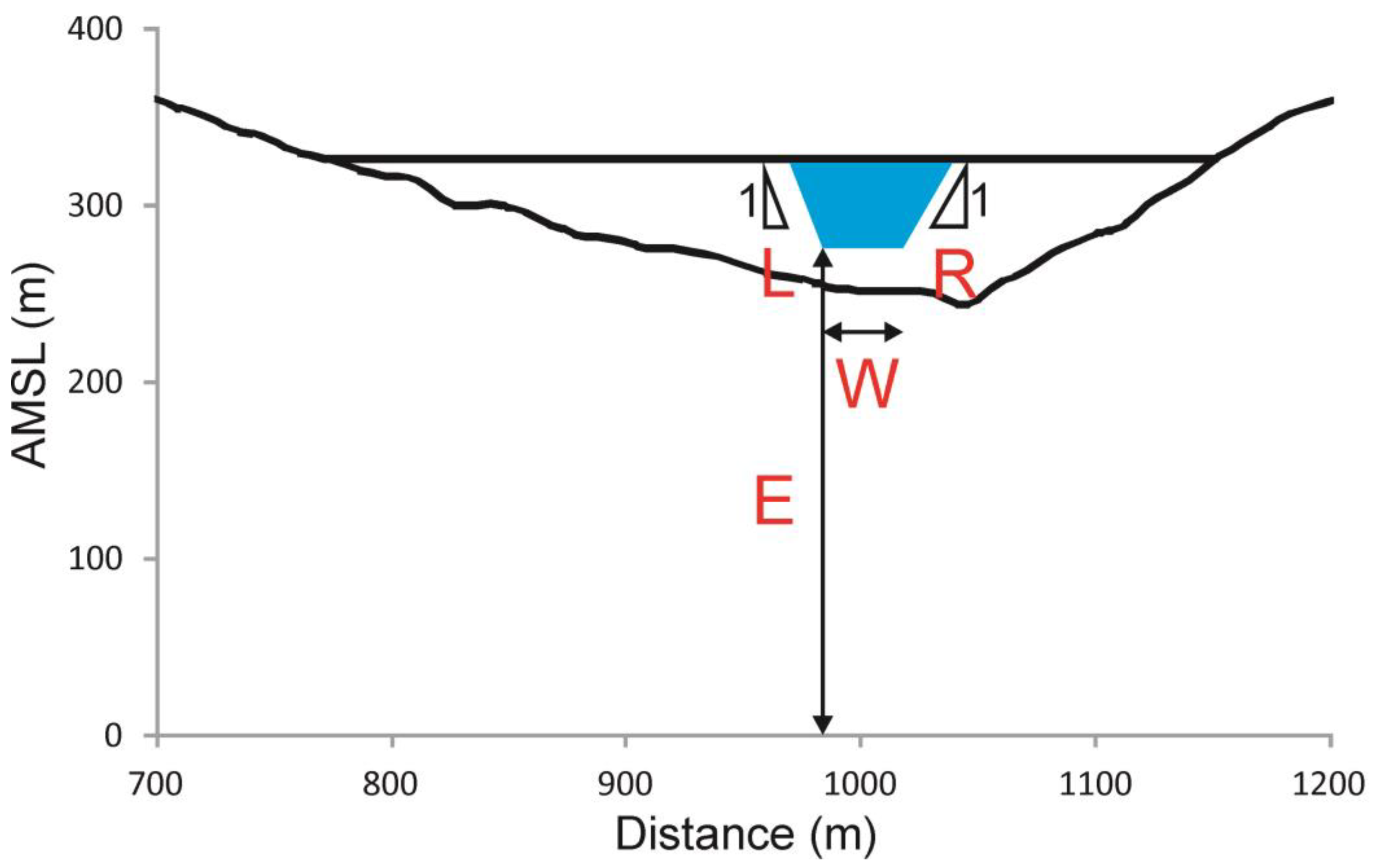
The breach modeling is implemented via the HEC-RAS software using the overtopping routine. In this option, the breach starts at the top and continues until the final shape of the breach, which is given by the modeler. The structure of the submodel is the weir coefficient and the input data is the Digital Terrain Model (DTM) of the reservoir (with a grid resolution of 5 m), which is used in order to derive the stage–volume curve. The required seven parameters of the submodel are the following:
- Final width of the breach at the bottom of the breach W
- Final elevation of the bottom of the breach E
- Left side slope of the breach L (H:V)
- Right side slope of the breach R (H:V)
- Breach weir coefficient c
- Required time for the completion of the breach t
- Water stage in the reservoir which triggers the failure S
Figure 2 depicts the cross-section of the dam and the geometrical characteristics of a typical dam breach.
With given geometrical characteristics of the final trapezoidal form of the breach (W, E, L, R) and the required time for that (t), breach shape can be defined with respect to time, using linear interpolation. Then, using the flow characteristics (weir coefficient c and water stage which triggers the failure S) and the input topography, outflow Q due to the failure can be calculated for every time moment using the weir equation:
where c is the breach weir coefficient, W is the width of the breach for each time moment, and H is the hydraulic head over the breach. The output derived by the above procedure is the flood hydrograph which is the input of the linked submodel, namely the hydrodynamic model.
2.3. Hydrodynamic Modeling
For the hydrodynamic submodel and the linkage with the breach submodel, HEC-RAS software is used as well. The selected model structure is the 1D unsteady routine, which is based on 1D-SWE, solved by the Finite Difference Method and the implicit box scheme. The reason for selecting the 1D instead of the 2D routine, which probably is characterized by less uncertainties, is mainly due to the computational burden which makes the sensitivity and uncertainty analysis unfeasible.
The input data consist of the flood hydrograph derived by the breach submodel, which is also the upstream boundary condition, and the DTM with a grid resolution of 5 m. Based on this DTM, cross-sections every 5 m are drawn along the 15 km of the river. It is noted that there is no topographic information in the subgrid scale of 5 m. However, this dense resolution of cross-sections is selected in order to encounter numerical instabilities, observed in coarser approaches.
For the downstream boundary condition, normal depth is selected, whilst the required energy slope is assumed to be equal to the average bottom slop of the stream, and specifically 0.02. Regarding the friction modeling, the entire computational domain is assumed to be homogeneous with a Manning coefficient equal to n = 0.2 s/m1/3. Although this consideration seems to be approximate, this unified value is selected because energy losses in such an extreme event due to turbulence are much bigger than the corresponding energy losses created due to roughness and with that implicit way, this is compensated [16,29].
For computational reasons, it is assumed that the initial discharge at the Tavronitis River reach, which is located downstream of Papadiana Dam, is equal to 100 m3/s, which is negligible in comparison with the flows observed after a hypothetical dam break. Finally, the time step is defined as equal to 10 s. It is noted that a preliminary investigation is performed in order to ensure that the selected time step does not affect the numerical solution.
2.4. Sensitivity Analysis
For the sensitivity analysis, a Morris-based algorithm is used [30]. The Morris screening method is included in Global Sensitivity Analysis methodologies and has been widely used in water-related problems [31,32,33]. The input in these types of methodologies is the range of the parameters which are under examination and selected variables from model results. The output of the method is two quantified variables, which denote the strongest influence and the nonlinearity effects on the results, respectively.
The core of the methodology is based on the calculation of the Elementary Effects (EE) for each input [34]. With a given parameter p, we can scale in the interval [0, 1] a given vector of input parameters (X1, X2, …, Xm) as {0, 1/(p-1), 2/(p-1), …, 1}. Now, the domain of the experiment Ω is an m-dimensional p-level grid. The EE for each input at a given point Χ in Ω can be calculated using the results of the model f(x), under the limitation that X+Δ belongs to Ω:
where Δ is a factor estimated by:
Following the next step of the methodology, we select the value of the trajectory r in order to define the final number of the required simulations N:
The final step of the methodology consists of calculating the mean μ and the standard deviation σ of the EE as follows:
The mean is a metric which quantifies the influence of each parameter. The higher the μ, the higher is the influence of the parameter on the variation of the result. The standard deviation is a metric which denotes the linearity. The higher the σ, the higher is the nonlinearity nature of the parameter.
In the present study, the sensitivity of the m = 7 breach parameters is examined, whilst three variables from the results are selected: (a) the flood peak of the hydrograph created in the dam location after the hypothetical failure; (b) flood peaks across the Tavronitis River; (c) maximum water depths across the Tavronitis River (water elevation minus minimum channel elevation). The number of trajectories selected is r = 50. Therefore, the number of required simulations (evaluations) for the sensitivity analysis is N = 400. The range of the breach parameters (Table 1) is selected using bibliographic values [35] and engineering judgment. The breach width ranges from 30 to 60% of the length of the dam, the breach height ranges from 65 to 85% of the dam height, and the water stage which triggers the failure corresponds to the 70–100% of the dam height.
2.5. Uncertainty Analysis
The uncertainty analysis performed in this paper is based on the Monte Carlo technique, which has been used by several researchers in the past [36,37] and can be summarized in the following steps:
- A plausible range of the parameters which are under examination is selected and a distribution of the sampling based on the prior knowledge is chosen.
- A large amount of random vectors of parameters is created based on the plausible range and the distribution of the sampling selected previously.
- Model simulations are performed having as an input the random vectors of the previous step.
- A variable drawn from the output of the model is selected in order to investigate its uncertainty.
- A distribution is fitted to the multiple outputs and the statistical characteristics of this distribution are estimated.
In this work, the parametric range was the same used for the sensitivity analysis (Table 1). Since there was no prior knowledge, uniform distribution was chosen. Based on the above, 10,000 random combinations of the seven parameters were drawn. The variables selected for the uncertainty analysis were the same as those used in sensitivity analysis, namely: (a) the flood peak of the hydrograph created at the dam location after the hypothetical failure; (b) flood peaks across the Tavronitis River; (c) maximum water depths across the Tavronitis River.
It should be noted that an investigation was made in order to ensure that we implemented a sufficient number of simulations. Specifically, in selected gauges, it was checked whether the statistical characteristics of the theoretical distributions used (normal and Weibull) became permanent towards the number of simulations. It was found that 10,000 simulations were capable of deriving reliable conclusions.
3. Results
3.1. Sensitivity Analysis
The sensitivity analysis was performed in three levels: (a) parametric influence on the flow peak of the hydrograph created due to dam failure; (b) parametric influence on the flow peak in the spatial scale, along the Tavronitis River; (c) parametric influence on the water depth maximum in the spatial scale, along the Tavronitis River. The parametric influence on the flow peak of the flood hydrograph at the dam location was visualized showing the mean of EES μ (the bigger value denotes the strongest influence) at the x axis and the standard deviation σ at the y axis (the bigger value denotes the bigger non linearity). For the parametric influence on the flow peaks and the maximum water depths along the Tavronitis River, the visualization was performed in three dimensions (3D plots): distance (x axis), mean of EEs (y axis), standard deviations of EEs (z axis).
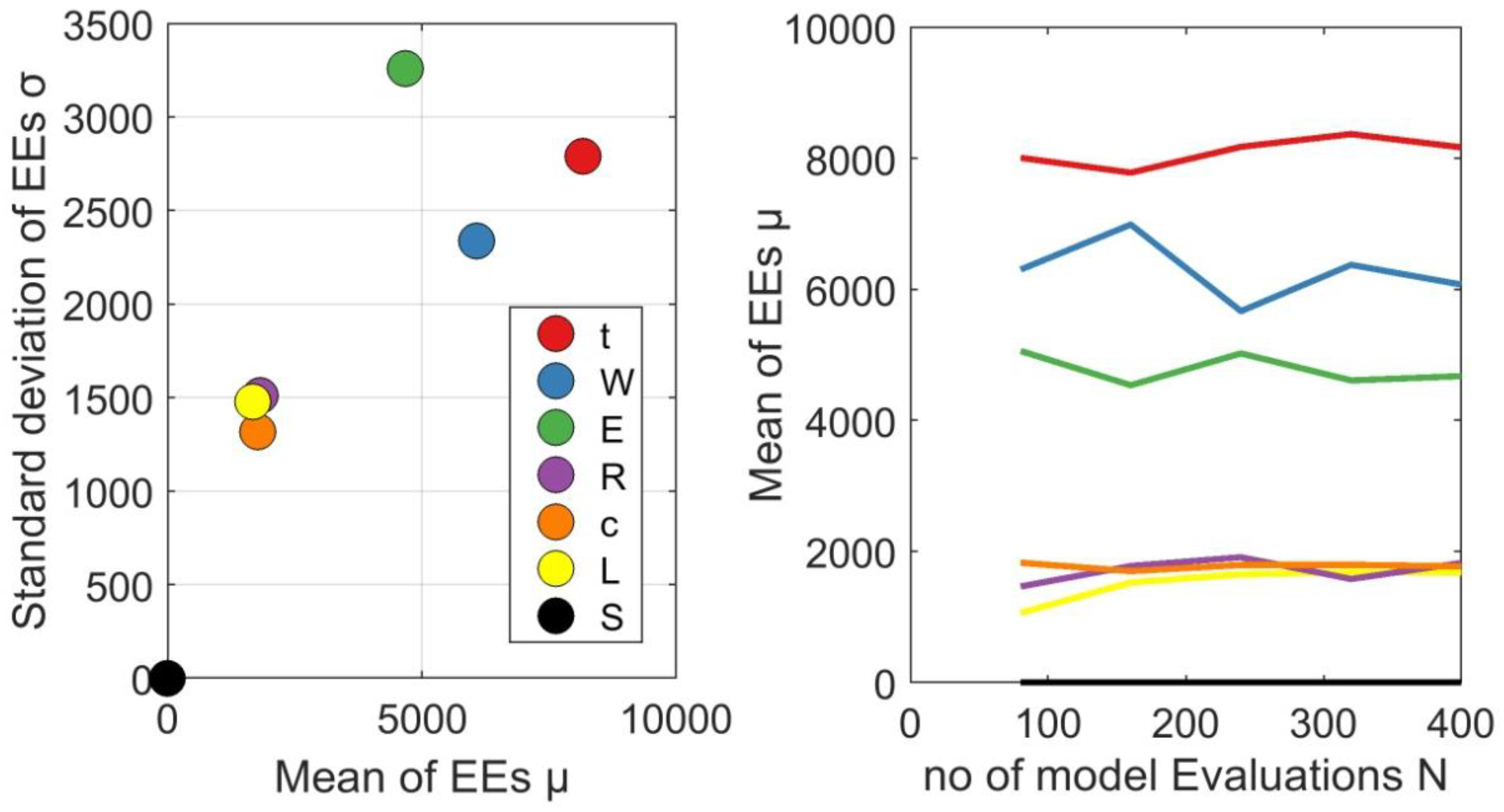
Figure 3 depicts the influence of each of the seven breach parameters on the flow peak of the flood hydrograph created at the dam location (left). At the right-hand side of the figure, the mean of EEs μ is shown with respect to the number of evaluations Ν, in order to investigate whether the final value of μ is not influenced by the number of evaluations.
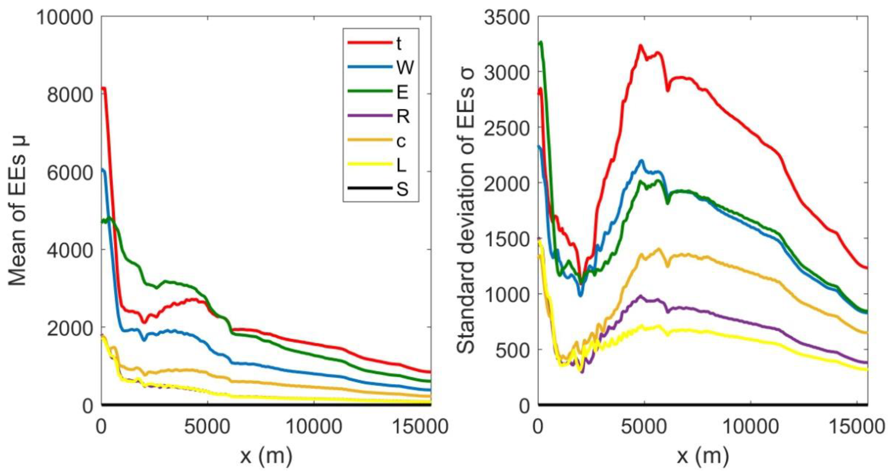
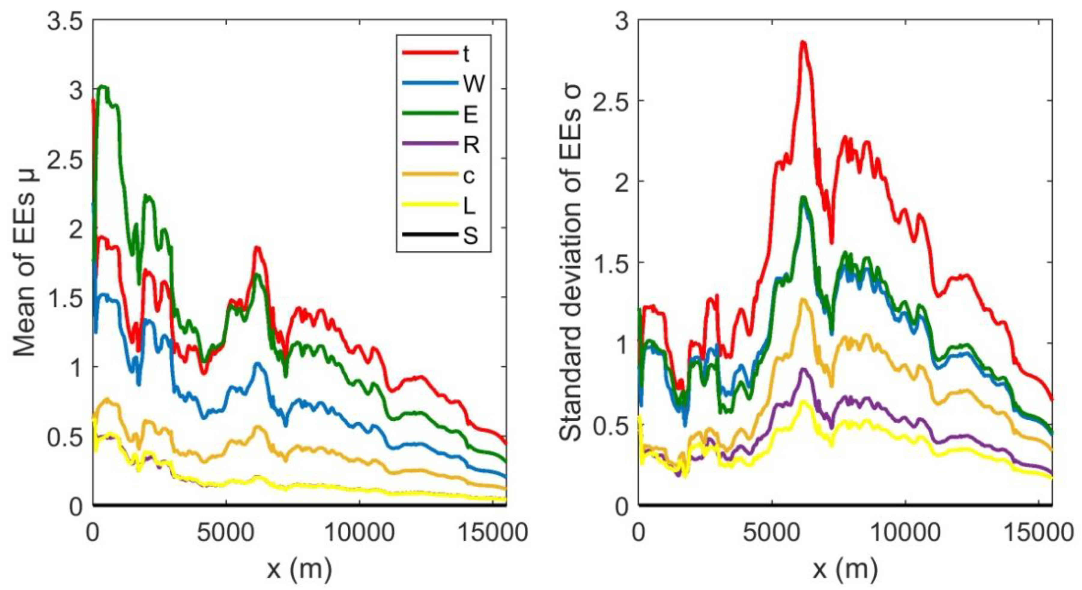
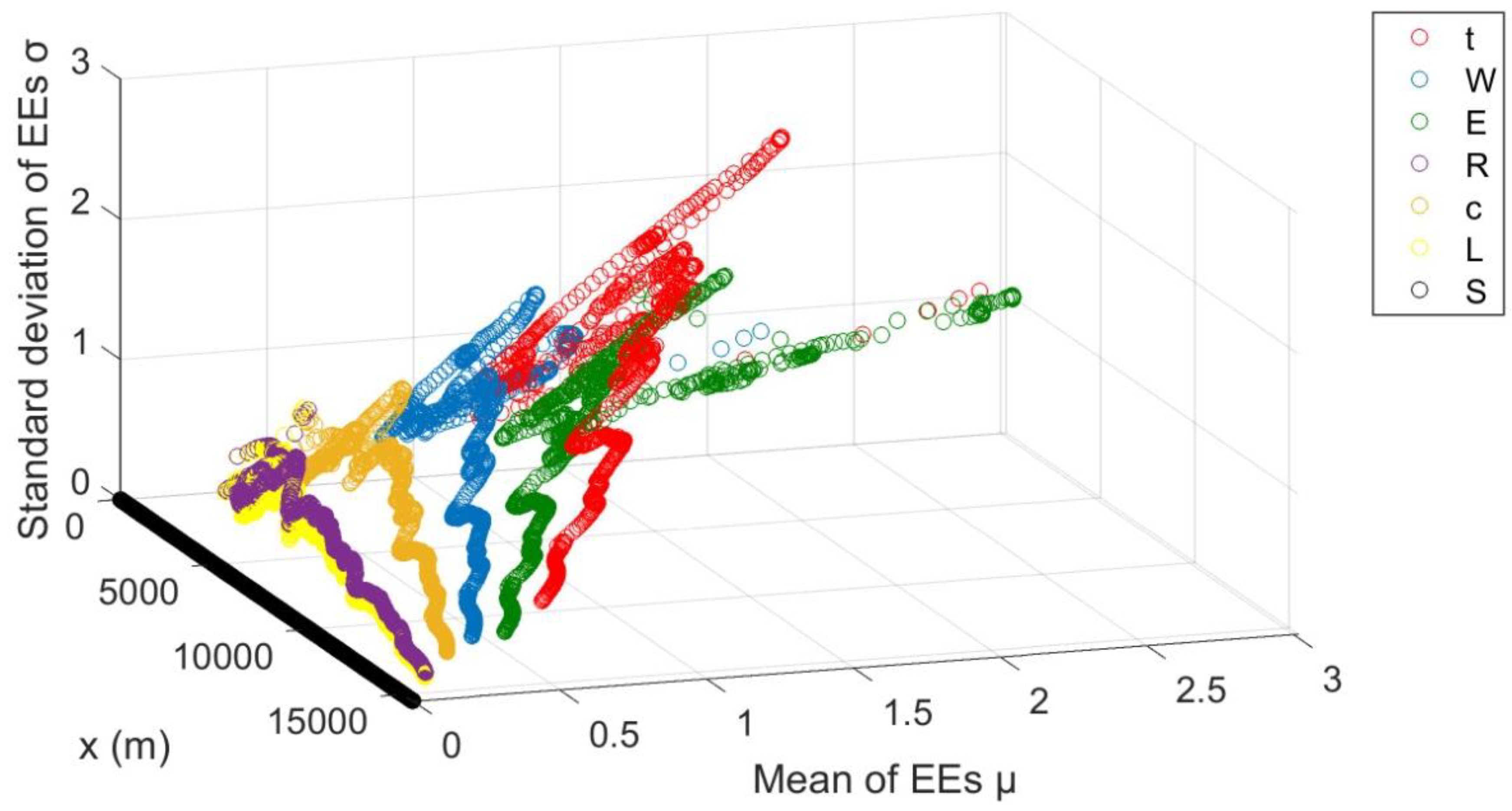
Figure 4 depicts the influence of each of the seven breach parameters on the flow peak (left) and the metric of nonlinearity (right) along the Tavronitis River. In Figure 5, the latter plots are merged into a 3D plot. The latter was applied to Figure 6 and Figure 7, for the maximum water depth.
It seems that the dam breach parameters can be classified into three groups (Figure 3, Figure 4, Figure 5, Figure 6 and Figure 7) according to their influence on the hydrodynamic results: (a) required time for the completion of the breach, final width of the breach at the bottom of the breach, final elevation of the bottom of the breach; (b) left and right side slope of the breach, breach weir coefficient; (c) water stage which triggers the failure.
The first group seemed to influence both flow peaks and maximum water depths at the spatial scale. The required time was the most sensitive parameter in the beginning (Figure 3) and in the end, but the rank between these three parameters varied along the river (left part of Figure 4 and Figure 6). The required time had a significant effect since the selected range was rather small, due to the fact that an RCC dam is expected to have a more rapid failure mechanism than an earthfill dam. The second group seemed to have a medium impact on the model outputs. Finally, the water stage which triggered the failure seemed to have a negligible impact. This was expected, since overtopping routine was selected, which means that initial water elevation when failure started was at the dam crest (the reservoir was full), whilst the breach started from the top of the dam. Therefore, this option is probably not required for future versions of HEC-RAS software.
Regarding the nonlinearity effects, it seems that in general there was a decreasing trend in space and besides, it was correlated with the sensitivity: the bigger the sensitivity, the stronger the nonlinearity (Figure 3, Figure 4 and Figure 6). A rather bizarre behavior for both flow peaks and maximum water depth, which requires further research, was that after a decreasing trend, a second peak of the standard deviation of EEs was observed in the middle of the stream. After that peak, the decreasing trend continued (right part of Figure 4 and Figure 6).
3.2. Uncertainty Analysis
As previously mentioned, just the parametric uncertainty of the dam breach submodel was examined. The output of this process was the input data for the hydrodynamic submodel. Uncertainty analysis was performed at three levels like sensitivity analysis: (a) for the dam location, the mean and the confidence intervals (75% and 95%) were derived with respect to the time, whilst for the 10,000 flow peaks, normal distribution was fitted; (b) for the flow peaks along the Tavronitis River, the Weibull distribution was fitted; (c) for the maximum water depths along the Tavronitis River, the Weibull distribution was fitted as well. It is noted that for the uncertainty analysis, MATLAB platform was used. Criteria for selecting a proper distribution were: (a) the performance of fitting should be good in the entire spatial scale of the river reach; (b) the theoretical distribution should be commonly used from the scientific community.
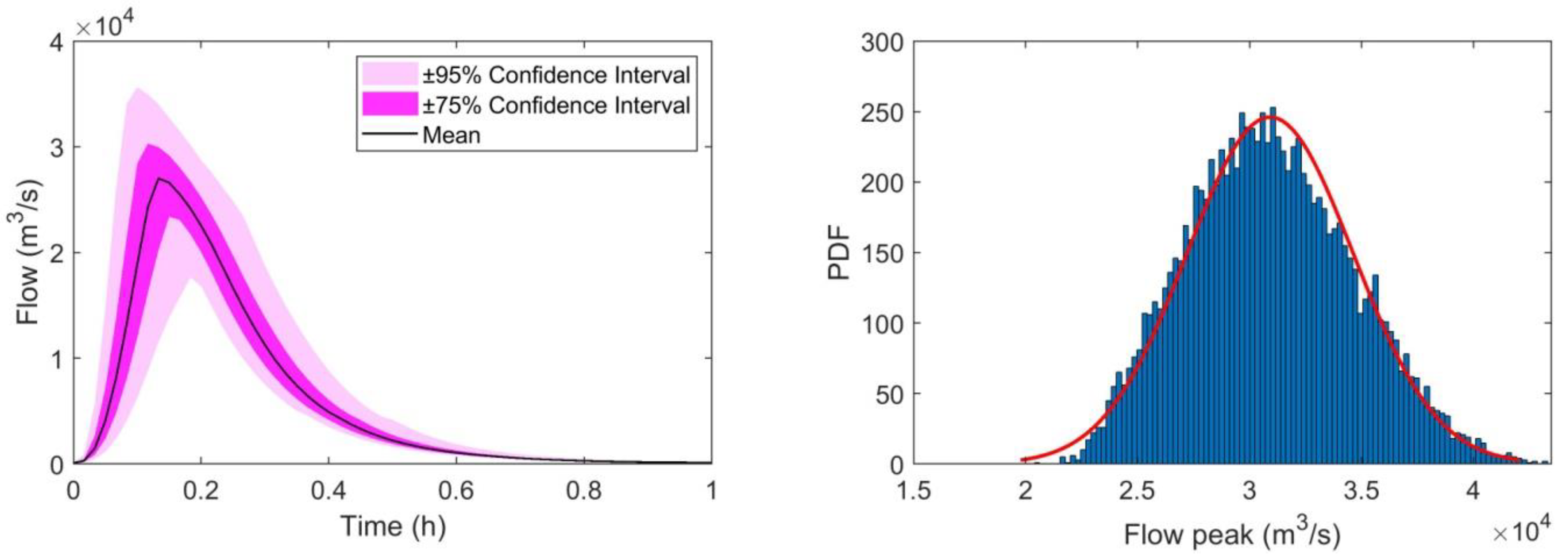
For the dam location, the uncertainty visualization is depicted in Figure 8: uncertainty band with respect to time (left) and normal distribution fitted to the results (right). The mean was calculated equal to m = 30,919.89 m3/s, whilst the standard deviation was equal to s = 3712.49 m3/s.
It seems that the uncertainty band is significant. The flood peak of the entire sample ranged from 20,560 to 43,280 m3/s, whilst the envelope of the ±95% confidence interval ranged from 25,040 to 37,280 m3/s. Besides, although the dam breach parameters were drawn assuming a uniform distribution (the seven parameters required for dam breach modeling), the normal distribution was fitted to the empirical distribution of the flow peaks of the flood hydrograph at the dam location, with a good performance.
In the next step, we selected a unique theoretical distribution for fitting the empirical distribution functions of maximum flows and water depths along the Tavronitis River, with a space step of 20 m. Taking into account the above criteria and by engineering judgment, the Weibull distribution was used, in which the Probability Density Function (PDF) was:
where κ, λ are parameters of the distribution. With these parameters, mean m and standard deviation s of the distribution can be calculated with the following equation:
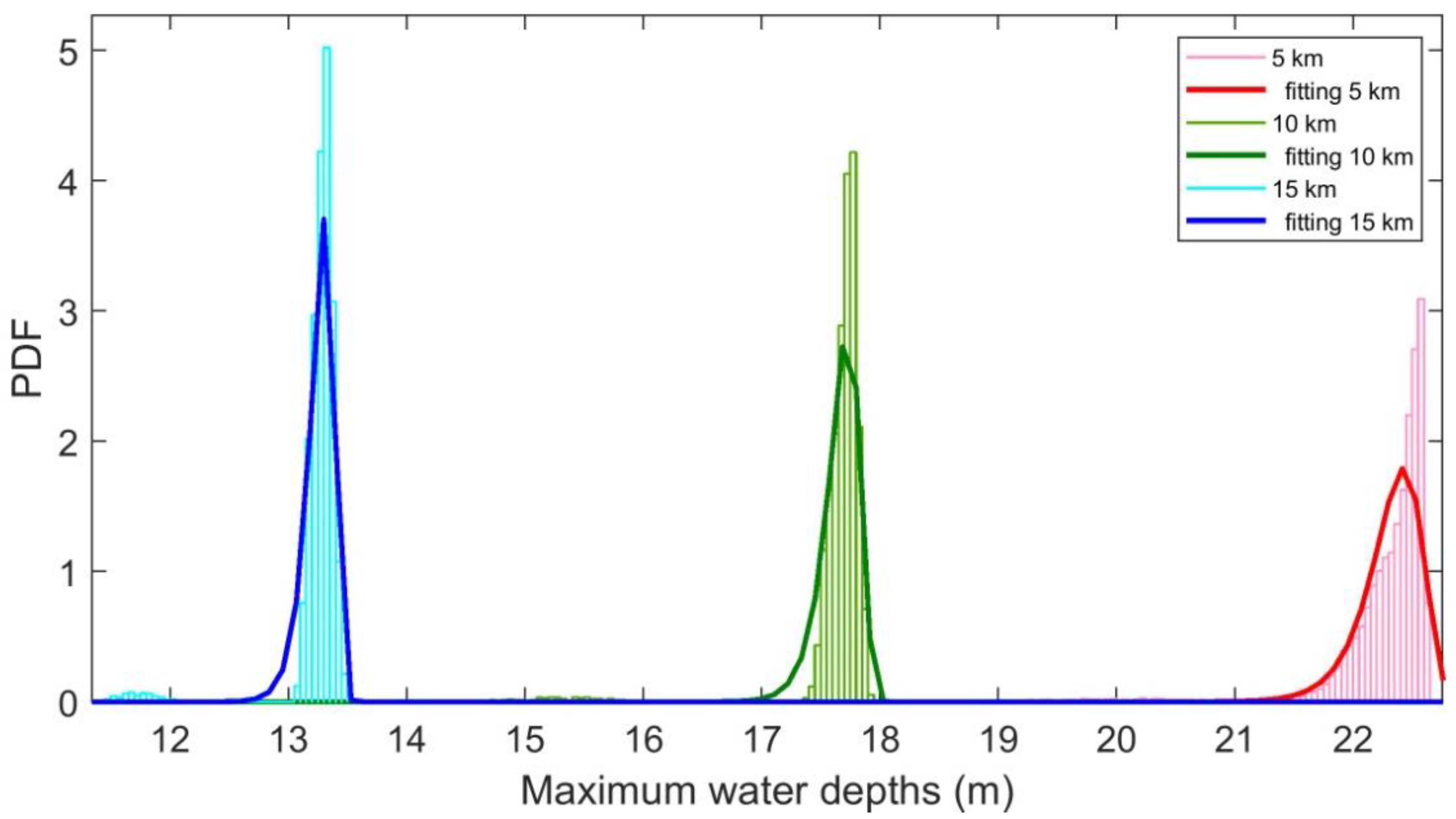
Figure 9 depicts the fitting of the flow peaks, in three indicative gauges (5 km, 10 km, and 15 km from the dam location), whilst Figure 10 depicts the fitting at the same gauges, but for the maximum water depths. From graphical observation, it seems that the fitting of the theoretical to the empirical distribution was good. There was a small discrepancy in the left tail of the distribution, especially in the cross-sections which are near the dam, which vanished in the outlet of the river to the sea.
A noticeable fact is that with a given input distribution which is nearly normal, skewness is observed at the empirical distributions of the flow peaks and the maximum water depths at the spatial scale. The latter has as a consequence that an extreme value distribution, such as Weibull distribution, is more appropriate for fitting to these empirical distributions.
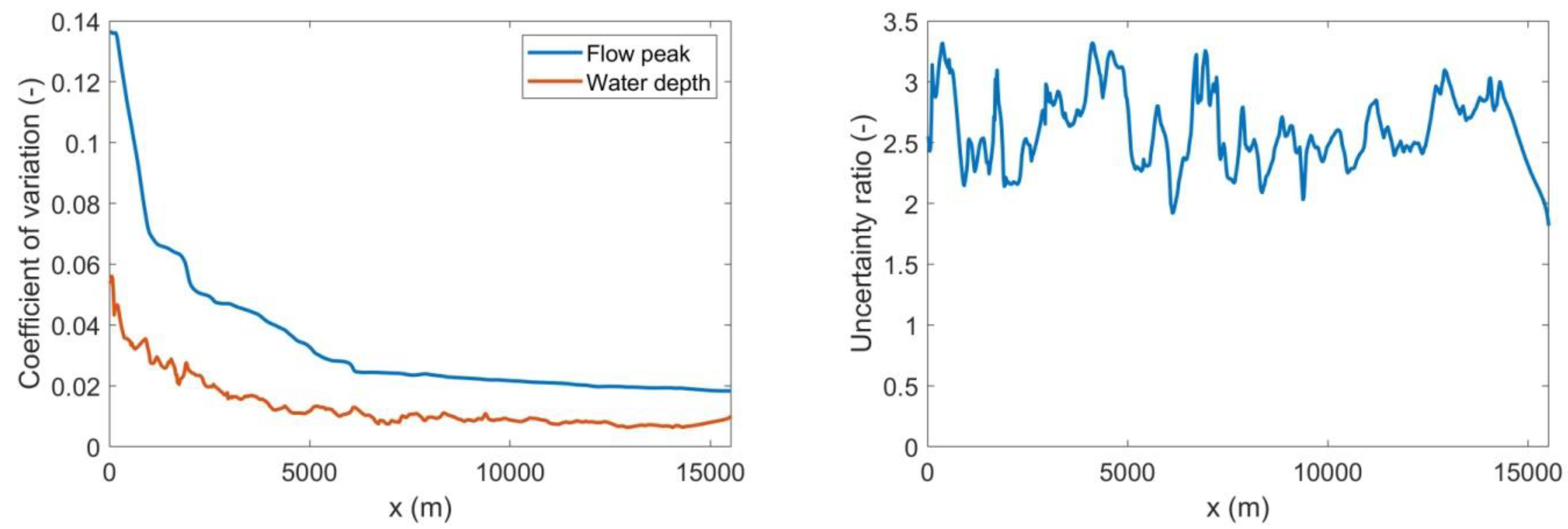
The coefficient of variation, namely the ratio s/m, can be used as a metric for the uncertainty to the model results due to the dam breach parameters. In order to investigate the propagation of this uncertainty, this coefficient was calculated along the Tavronitis River and is depicted in Figure 11, for both peak flows and maximum water depths (left). Besides, the ratio of the flow peak uncertainty to the maximum water depth uncertainty was also calculated (Figure 11, right).
Although the uncertainty band for all the levels (flood hydrograph at the dam location, flow peaks and maximum water depths along the stream) seemed to be significant, there was a clear decreasing trend of the uncertainty along the space, for both flow peaks and maximum water depths (left part of Figure 11). It seems that the mechanism of energy losses, which is also responsible for the natural diffusion effects at the flood wave which is propagated through the spatial scale, compensates the uncertainties created due to the dam breach parameters range along the river. This is also discussed in [7].
The uncertainty observed at the flow peaks was systematically bigger than the uncertainty observed at the maximum water depths (right part of Figure 11). In this specific case study, it was about 2.5. This is expected, due to the fact that the momentum equation of 1D-SWE (with which flow is derived) is nonlinear, whilst the continuity equation of 1D-SWE (with which water depth is derived) is linear.
4. Discussion and Concluding Remarks
First, it should be noted that our analysis was made in an ad hoc real-world case study, namely the Papadiana Dam, Crete, Greece, which is characterized by significant complexities. Besides, just a single hydrodynamic software was used, namely the HEC-RAS software, which also has its uncertainties. Therefore, it is not in our intentions to state global conclusions. However, there are some remarkable findings which require further research.
Seven breach parameters were examined for three levels of uncertainty: (a) at the flood hydrograph created at the dam location; (b) the flow peaks along the river; (c) the maximum water depths along the river. For the uncertainty analysis, two methods were used: (a) a Morris-based method for defining the impact of each parameter on the latter levels and (b) a Monte Carlo-based method which fits theoretical distributions and calculates its statistical characteristics, at the empirical distributions of the three levels of uncertainty.
First, it was found that uncertainty issues are significant and this should be taken into account by modelers and engineers at the design stage. The uncertainty band of the flow peak was about 25,000 m3/s. In fact, we probably would find just as big a number in order to investigate the consequences of a potential flood created by a dam failure.
Second, it was found that a uniform distribution input in the dam breach submodel derives an output which is close to the normal distribution. In turn, this output, which is the input for the hydrodynamic submodel, derives an output with skewness, which is closer to an extreme value theoretical distribution, such as Weibull distribution used in this paper.
Third, it was found that regarding their impact on the final results, the dam breach parameters can be classified into three groups with significant, medium, and negligible impact. The first group which has the most significant impact consists of the required time for the completion of the breach, the final width at the bottom of the breach, and the final elevation of the bottom of the breach.
Finally, it was found that there is a clear decreasing trend of uncertainty along the river downstream of the dam. In fact, this uncertainty is the input data uncertainty for the hydrodynamic submodel, which is the output of the parametric uncertainty of the dam breach submodel. This can be explained by the fact that the natural mechanism of diffusion compensates uncertainties at the spatial scale. Besides, there is a systematic ratio between the uncertainties observed at the flow peaks and the uncertainties observed at the maximum water depths, which is equal to about 2.5.
Author Contributions
Conceptualization, V.B.; methodology, V.B.; software, V.B., V.K.T. and G.K., data curation, V.K.T; writing—original draft preparation, V.B.; writing—review and editing, V.B. and G.T.; visualization, V.B. and G.K.; supervision, G.T.; project administration, G.T.; funding acquisition, V.B. and G.T. All authors have read and agreed to the published version of the manuscript.
Funding
This research was partially funded by the Region of Crete, grant number 17SYMV001593629, and partially from the Greek State Scholarships Foundation, grant number 2019-050-0503-17909.
Acknowledgments
Vasilis Bellos is grateful to the Greek State Scholarships Foundation (IKY) for funding part of this work. More specifically: this research is co-financed by Greece and the European Union (European Social Fund-ESF) through the Operational Programme «Human Resources Development, Education and Lifelong Learning» in the context of the project “Reinforcement of Postdoctoral Researchers—2nd Cycle” (MIS-5033021), implemented by the State Scholarships Foundation (ΙΚΥ).
Conflicts of Interest
The authors declare no conflict of interest.
References
- Bosa, S.; Petti, M. A Numerical Model of the Wave that Overtopped the Vajont Dam in 1963. Water Resour. Manag. 2013, 27, 1763–1779. [Google Scholar] [CrossRef]
- Duffaut, P. The traps behind the failure of Malpasset arch dam, France, in 1959. J. Rock Mech. Geotech. Eng. 2013, 5, 335–341. [Google Scholar] [CrossRef] [Green Version]
- Arthur, H. Teton Dam Failure. In Proceedings of the Engineering Foundation Conference, Pacific Grove, CA, USA, 28 November–3 December 1976; pp. 61–68. [Google Scholar]
- Micah, S.M. Amazon.com: The Ecology of War in China: Henan Province, the Yellow River, and Beyond, 1938–1950 (Studies in Environment and History) (9781107071568). Available online: https://www.amazon.com/Ecology-War-China-1938-1950-Environment/dp/1107071569 (accessed on 22 July 2020).
- Tsakiris, G.; Bellos, V.; Ziogas, C. Embankment Dam Failure: A Downstream Flood Hazard Assessment. Eur. Water 2010, 32, 35–45. [Google Scholar]
- Schulz, C.; Martin-Ortega, J.; Glenk, K. Understanding Public Views on a Dam Construction Boom: The Role of Values. Water Resour. Manag. 2019, 33, 4687–4700. [Google Scholar] [CrossRef] [Green Version]
- Tscheikner-Gratl, F.; Bellos, V.; Schellart, A.; Moreno-Rodenas, A.; Muthusamy, M.; Langeveld, J.; Clemens, F.; Benedetti, L.; Rico-Ramirez, M.A.; de Carvalho, R.F.; et al. Recent insights on uncertainties present in integrated catchment water quality modelling. Water Res. 2019, 150, 368–379. [Google Scholar] [CrossRef] [PubMed]
- MacDonald, T.C.; Langridge-Monopolis, J. Breaching Charateristics of Dam Failures. J. Hydraul. Eng. 1984, 110, 567–586. [Google Scholar] [CrossRef]
- Froehlich, D.C. Embankment Dam Breach Parameters and Their Uncertainties. J. Hydraul. Eng. 2008, 134, 1708–1721. [Google Scholar] [CrossRef]
- Macchione, F. Model for Predicting Floods due to Earthen Dam Breaching. I: Formulation and Evaluation. J. Hydraul. Eng. 2008, 134, 1688–1696. [Google Scholar] [CrossRef]
- Xu, Y.; Zhang, L.M. Breaching Parameters for Earth and Rockfill Dams. J. Geotech. Geoenviron. Eng. 2009, 135, 1957–1970. [Google Scholar] [CrossRef]
- Tsakiris, G.; Spiliotis, M. Dam- Breach Hydrograph Modelling: An Innovative Semi- Analytical Approach. Water Resour. Manag. 2013, 27, 1751–1762. [Google Scholar] [CrossRef]
- Valiani, A.; Caleffi, V.; Zanni, A. Case Study: Malpasset Dam-Break Simulation using a Two-Dimensional Finite Volume Method. J. Hydraul. Eng. 2002, 128, 460–472. [Google Scholar] [CrossRef]
- Begnudelli, L.; Sanders, B.F. Simulation of the St. Francis Dam-Break Flood. J. Eng. Mech. 2007, 133, 1200–1212. [Google Scholar] [CrossRef]
- El Kadi Abderrezzak, K.; Paquier, A.; Mignot, E. Modelling flash flood propagation in urban areas using a two-dimensional numerical model. Nat. Hazards 2009, 50, 433–460. [Google Scholar] [CrossRef]
- Bellos, V.; Tsakiris, G. 2D Flood Modelling: The case of Tous Dam Break. In Proceedings of the 36th of IAHR World Congress, Hague, The Netherlands, 28 June–3 July 2015. [Google Scholar]
- Petaccia, G.; Natale, L. 1935 Sella Zerbino Dam-Break Case Revisited: A New Hydrologic and Hydraulic Analysis. J. Hydraul. Eng. 2020, 146, 05020005. [Google Scholar] [CrossRef]
- Alcrudo, F.; Mulet, J. Description of the Tous Dam break case study (Spain). J. Hydraul. Res. 2007, 45, 45–57. [Google Scholar] [CrossRef]
- Fread, D.L. NWS FLDWAV Model: Theoretical Description; Hydrologic Research Laboratory, Office of Hydrology, National Weather Service, NOAA: Washington, DC, USA, 1998.
- Bladé, E.; Cea, L.; Corestein, G.; Escolano, E.; Puertas, J.; Vázquez-Cendón, E.; Dolz, J.; Coll, A. Iber: Herramienta de simulación numérica del flujo en ríos. Rev. Int. Métodos Numér. Cálc. Diseño Ing. 2014, 30, 1–10. [Google Scholar] [CrossRef] [Green Version]
- HEC-RAS. River Analysis System Hydraulic Reference Manual; Hydrologic Engineering Center US Army Corps of Engineer: Davis, CA, USA, 2016.
- Macchione, F.; Costabile, P.; Costanzo, C.; De Lorenzo, G.; Razdar, B. Dam breach modelling: Influence on downstream water levels and a proposal of a physically based module for flood propagation software. J. Hydroinform. 2016, 18, 615–633. [Google Scholar] [CrossRef]
- Haltas, I.; Elçi, S.; Tayfur, G. Numerical Simulation of Flood Wave Propagation in Two-Dimensions in Densely Populated Urban Areas due to Dam Break. Water Resour. Manag. 2016, 30, 5699–5721. [Google Scholar] [CrossRef] [Green Version]
- Pilotti, M.; Milanesi, L.; Bacchi, V.; Tomirotti, M.; Maranzoni, A. Dam-Break Wave Propagation in Alpine Valley with HEC-RAS 2D: Experimental Cancano Test Case. J. Hydraul. Eng. 2020, 146, 05020003. [Google Scholar] [CrossRef]
- Kim, B.; Sanders, B.F. Dam-Break Flood Model Uncertainty Assessment: Case Study of Extreme Flooding with Multiple Dam Failures in Gangneung, South Korea. J. Hydraul. Eng. 2016, 142, 05016002. [Google Scholar] [CrossRef]
- Albu, L.-M.; Enea, A.; Iosub, M.; Breabăn, I.-G. Dam Breach Size Comparison for Flood Simulations. A HEC-RAS Based, GIS Approach for Drăcșani Lake, Sitna River, Romania. Water 2020, 12, 1090. [Google Scholar] [CrossRef]
- Kalinina, A.; Spada, M.; Vetsch, D.F.; Marelli, S.; Whealton, C.; Burgherr, P.; Sudret, B. Metamodeling for Uncertainty Quantification of a Flood Wave Model for Concrete Dam Breaks. Energies 2020, 13, 3685. [Google Scholar] [CrossRef]
- Lee, J.-S.; Noh, J.W. The impacts of uncertainty in the predicted dam breach floods on economic damage estimation. KSCE J. Civ. Eng. 2003, 7, 343–350. [Google Scholar] [CrossRef]
- Bellos, V.; Nalbantis, I.; Tsakiris, G. Friction Modeling of Flood Flow Simulations. J. Hydraul. Eng. 2018, 144, 04018073. [Google Scholar] [CrossRef] [Green Version]
- Pianosi, F.; Sarrazin, F.; Wagener, T. A Matlab toolbox for Global Sensitivity Analysis. Environ. Model. Softw. 2015, 70, 80–85. [Google Scholar] [CrossRef] [Green Version]
- Christelis, V.; Hughes, A.G. Metamodel-assisted analysis of an integrated model composition: An example using linked surface water–groundwater models. Environ. Model. Softw. 2018, 107, 298–306. [Google Scholar] [CrossRef] [Green Version]
- Sriwastava, A.K.; Tait, S.; Schellart, A.; Kroll, S.; Dorpe, M.V.; Assel, J.V.; Shucksmith, J. Quantifying Uncertainty in Simulation of Sewer Overflow Volume. J. Environ. Eng. 2018, 144, 04018050. [Google Scholar] [CrossRef] [Green Version]
- Bellos, V.; Papageorgaki, I.; Kourtis, I.; Vangelis, H.; Kalogiros, I.; Tsakiris, G. Reconstruction of a flash flood event using a 2D hydrodynamic model under spatial and temporal variability of storm. Nat. Hazards 2020, 101, 711–726. [Google Scholar] [CrossRef]
- Morris, M.D. Factorial Sampling Plans for Preliminary Computational Experiments. Technometrics 1991, 33, 161–174. [Google Scholar] [CrossRef]
- Federal Energy Regulatory Commission. Chapter 2: Selecting and Accommodating Inflow Design Floods for Dams; Federal Energy Regulatory Commission: Washington, DC, USA, 2015.
- Dimitriadis, P.; Tegos, A.; Oikonomou, A.; Pagana, V.; Koukouvinos, A.; Mamassis, N.; Koutsoyiannis, D.; Efstratiadis, A. Comparative evaluation of 1D and quasi-2D hydraulic models based on benchmark and real-world applications for uncertainty assessment in flood mapping. J. Hydrol. 2016, 534, 478–492. [Google Scholar] [CrossRef]
- Bellos, V.; Kourtis, I.M.; Moreno-Rodenas, A.; Tsihrintzis, V.A. Quantifying Roughness Coefficient Uncertainty in Urban Flooding Simulations through a Simplified Methodology. Water 2017, 9, 944. [Google Scholar] [CrossRef] [Green Version]
Figure 1.
Location of Papadiana Dam, Crete island, Greece.

Figure 2.
Cross-section of Papadiana dam and typical dam breach geometrical characteristics.

Figure 3.
Metric of influence (mean of EEs) and metric of nonlinearity (standard deviations of EEs) (left); mean of EEs with respect to the evaluation number (right).
Figure 3.
Metric of influence (mean of EEs) and metric of nonlinearity (standard deviations of EEs) (left); mean of EEs with respect to the evaluation number (right).

Figure 4.
Metric of influence (mean of EEs) along space (left) and metric of nonlinearity (standard deviations of EEs) along space (right), for flow peaks.
Figure 4.
Metric of influence (mean of EEs) along space (left) and metric of nonlinearity (standard deviations of EEs) along space (right), for flow peaks.

Figure 5.
A merged 3D plot: distance (x axis), mean of EEs (y axis), standard deviations of EEs (z axis) for flow peaks.
Figure 5.
A merged 3D plot: distance (x axis), mean of EEs (y axis), standard deviations of EEs (z axis) for flow peaks.

Figure 6.
Metric of influence (mean of EEs) along space (left) and metric of nonlinearity (standard deviations of EEs) along space (right), for maximum water depth.
Figure 6.
Metric of influence (mean of EEs) along space (left) and metric of nonlinearity (standard deviations of EEs) along space (right), for maximum water depth.

Figure 7.
A merged 3D plot: distance (x axis), mean of EEs (y axis), standard deviations of EEs (z axis) for maximum water depths.
Figure 7.
A merged 3D plot: distance (x axis), mean of EEs (y axis), standard deviations of EEs (z axis) for maximum water depths.

Figure 8.
Uncertainty band and confidence intervals for the flood hydrograph created after the dam break (left); fitting normal distribution at the 10,000 flow peaks of the flood hydrographs (right).
Figure 8.
Uncertainty band and confidence intervals for the flood hydrograph created after the dam break (left); fitting normal distribution at the 10,000 flow peaks of the flood hydrographs (right).

Figure 9.
Weibull distribution fitting in three indicative gauges, for flow peaks.

Figure 10.
Weibull distribution fitting in three indicative gauges, for maximum water depths.

Figure 11.
Coefficient of variation in the spatial scale for both flow peaks and maximum water depths (left); ratio of the coefficient of variation of the flow peak to the coefficient of variation of the maximum water depth along the stream (right).
Figure 11.
Coefficient of variation in the spatial scale for both flow peaks and maximum water depths (left); ratio of the coefficient of variation of the flow peak to the coefficient of variation of the maximum water depth along the stream (right).


Table 1.
Range of breach parameters
| Parameter | Description | Range | Unit |
|---|---|---|---|
| W | breach width | 100–200 | m |
| E | bottom elevation of the breach (AMSL) | 251–270 | m |
| L | left side slope of the breach | 0–2 | - |
| R | right side slope of the breach | 0–2 | - |
| c | breach weir coefficient | 1.2–1.6 | m1/2/s |
| t | required time | 0.2–0.5 | h |
| S | water stage which triggers the failure (AMSL) | 300–326 | m |
© 2020 by the authors. Licensee MDPI, Basel, Switzerland. This article is an open access article distributed under the terms and conditions of the Creative Commons Attribution (CC BY) license (http://creativecommons.org/licenses/by/4.0/).
Share and Cite
MDPI and ACS Style
Bellos, V.; Tsakiris, V.K.; Kopsiaftis, G.; Tsakiris, G. Propagating Dam Breach Parametric Uncertainty in a River Reach Using the HEC-RAS Software. Hydrology 2020, 7, 72. https://0-doi-org.brum.beds.ac.uk/10.3390/hydrology7040072
AMA Style
Bellos V, Tsakiris VK, Kopsiaftis G, Tsakiris G. Propagating Dam Breach Parametric Uncertainty in a River Reach Using the HEC-RAS Software. Hydrology. 2020; 7(4):72. https://0-doi-org.brum.beds.ac.uk/10.3390/hydrology7040072
Chicago/Turabian StyleBellos, Vasilis, Vasileios Kaisar Tsakiris, George Kopsiaftis, and George Tsakiris. 2020. "Propagating Dam Breach Parametric Uncertainty in a River Reach Using the HEC-RAS Software" Hydrology 7, no. 4: 72. https://0-doi-org.brum.beds.ac.uk/10.3390/hydrology7040072
Note that from the first issue of 2016, this journal uses article numbers instead of page numbers. See further details here.