Predicting Runoff Chloride Concentrations in Suburban Watersheds Using an Artificial Neural Network (ANN)


Department of Geosciences, University of Rhode Island, 315 Woodward Hall, 9 E. Alumni Ave, Kingston, RI 02881, USA
*
Author to whom correspondence should be addressed.
Hydrology 2020, 7(4), 80; https://0-doi-org.brum.beds.ac.uk/10.3390/hydrology7040080
Submission received: 26 August 2020
/
Revised: 30 September 2020
/
Accepted: 13 October 2020
/
Published: 21 October 2020
Abstract
:Road salts in stormwater runoff, from both urban and suburban areas, are of concern to many. Chloride-based deicers [i.e., sodium chloride (NaCl), magnesium chloride (MgCl2), and calcium chloride (CaCl2)], dissolve in runoff, travel downstream in the aqueous phase, percolate into soils, and leach into groundwater. In this study, data obtained from stormwater runoff events were used to predict chloride concentrations and seasonal impacts at different sites within a suburban watershed. Water quality data for 42 rainfall events (2016–2019) greater than 12.7 mm (0.5 inches) were used. An artificial neural network (ANN) model was developed, using measured rainfall volume, turbidity, total suspended solids (TSS), dissolved organic carbon (DOC), sodium, chloride, and total nitrate concentrations. Water quality data were trained using the Levenberg-Marquardt back-propagation algorithm. The model was then applied to six different sites. The new ANN model proved accurate in predicting values. This study illustrates that road salt and deicers are the prime cause of high chloride concentrations in runoff during winter and spring, threatening the aquatic environment.
1. Introduction
Urban areas require the construction of buildings, roads, and parking areas, yet such urban development causes hydrologic impacts and pollution as pervious surfaces are made impervious [1]. For safety, given abundant snowfall during the winter season, most communities in New England use salt or deicing on roads and parking areas. Road salts or deicing during the winter season are the primary factors for increasing salinity in surface soils, surface water, groundwater, and runoff. In the USA, an average of 24 million metric tons of road salt is applied each year to roads [2]. It is well-established that the application of road salts leads to the accumulation of sodium and chloride in soils and surface waters [3,4,5], with adverse impacts on downstream aquatic ecosystems [6]. In fact, when impervious surface areas increase, the areas that need to be deiced also increase.
Chloride-based deicers [i.e., sodium chloride (NaCl), magnesium chloride (MgCl2), and calcium chloride (CaCl2)] dissolve in runoff, percolate into soils, and leach into groundwater. Chloride from chloride-based deicers does not efficiently precipitate or biodegrade but is absorbed by mineral/soil surfaces [7]. Although winter road deicing is an essential service for urban areas in USA (especially in the upper Midwest and Northeast), it contributes to a significant increase in chloride concentration [8]. The United States Geological Survey (USGS) (2014) conducted a temporal, seasonal, and environmental analysis of chloride concentrations in urban areas and assessed effects on water quality and the environment, especially on aquatic organisms across the USA [8]. This study concluded that there is an increasing trend of high chloride concentrations in urban areas due to expansion of impervious cover that requires deicing.
An increasing trend in chloride concentrations in some US rivers is shown in Figure 1 and attributed to increased usage of road salt; the trend is positive in New England (USGS, 2014). The increasing salinity not only threatens aquatic ecosystems, but also contributes to corrosion in water distribution systems. Salinity can increase even with little snowfall due to efficient transfer of chloride to wastewater discharge or septic systems [8]. Areas that have no snow, such as Florida, also showed increasing salinity. In the case of Florida, less than normal rainfall since 1990 combined with groundwater level decline due to over pumping explain the observed increasing salinity [9,10,11]. The characteristics and degradation of urban runoff quality and its impact on the environment largely depend on the urban land-use practices, site geology, and hydrogeology. The large quantity of road salt that is applied every year for snow removal in the USA is one of the major contributors to declining stormwater quality.
Recently, several studies have applied artificial neural network (ANN) methods to predict resulting water quality based upon input variables [12]. Since 1990, ANN has been applied in many fields, including environmental sciences, ecological sciences, and water engineering [13]. According to Haykin (1999) [14], ANN is highly capable in modeling nonlinear system estimation and is highly adaptable. ANN allows precise predictions of the target parameter for specific materials or stages [14,15].
In this study, an ANN model is developed with a back-propagation algorithm. The back-propagation algorithm incorporates highly nonlinear relationships [15]. The ANN model was developed for rapid calculation and prediction of selected water quality variables at any location of interest. Within the model, unknown parameter weights are adjusted to obtain the best correlation between appropriate input parameters or a historical set of model inputs and the corresponding outputs [16]. This study provides the ANN modeling method needed to simulate and forecast chloride concentrations in runoff. The aim of the study is to (i) develop an ANN model of the system trained using a small data set, (ii) obtain the best-fit models for predicting chloride concentrations using data from monitoring sites, (iii) evaluate the ANN model performance using 3 years (2016–2019) of observed data versus predicted data from the model, and (iv) determine the accuracy of the ANN model performance. The model also assesses the impact of road salt applications through assessment of a spatial density distribution focused on probable high chloride concentration in an area.
2. Materials and Methods
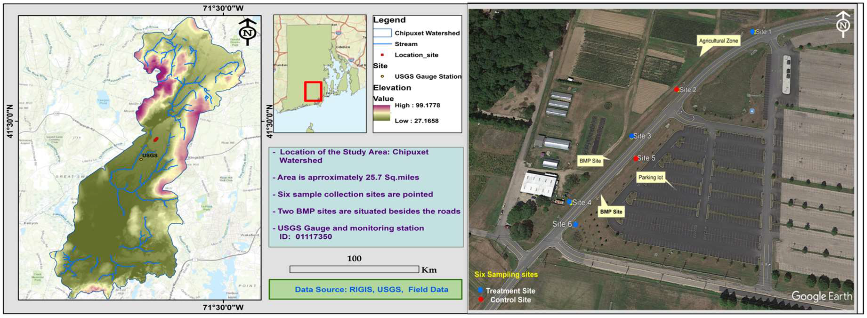
A three-year study on the effectiveness of the stormwater best management practices (BMPs) was conducted in the Chipuxet watershed of South Kingstown, Rhode Island, USA (Figure 2).
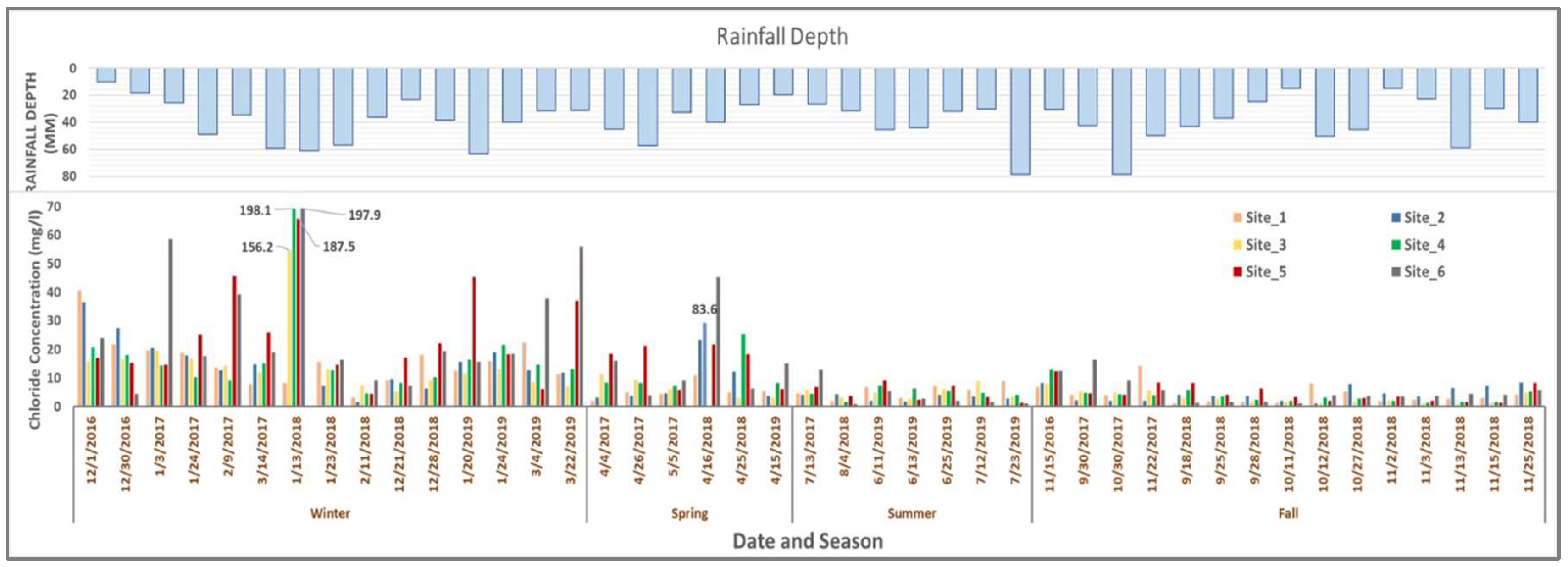
An overview of the chloride concentration for three years (2016–2019) from six sites represented in Figure 3. Based on the analysis of the stormwater runoff quality data, an apparent seasonal variation of chloride concentration is observed (Figure 3). The higher concentration of chloride was found during winter and early spring season (at the tail end of winter). Our study results are highly consistent with the study conducted by the USGS (2014) [7]. The USGS study showed the increasing trend of chloride concentration in the New England zone, and our data also provided the same impression. As stated above, high chloride concentration (0.8–197.9) mg/L was seen on the winter samples for all the sites. Site 5 and 6 are in close proximity to the parking lot; parking lots are highly impermeable, and exhibited higher chloride concentration (0.9–197.9) mg/L than the remaining four sites that are close to the agricultural field (Figure 3). The chloride concentration data were then used to investigate the future scenario through the ANN model. The steps used to develop the model include the choice of model performance criteria, preprocessing of available data, the selection of appropriate model inputs, and network structure.
2.1. Artificial Neural Network (ANN)
The ANN concept was first introduced by McCulloch and Pits in 1943, and ANN applications in research areas started with the back-propagation algorithm for feed-forward ANN in 1986 [17,18]. ANNs consist of multiple layers; basic layers are common to all models (i.e., input layer, output layer), and several hidden layers may be needed (located between the input and output of the algorithm) [19]. Each of the layers in an ANN consists of a parameterizable number of neurons. Neurons are activation functions of adjustable weight based on a priori and domain knowledge [20]. In this study, an ANN with three different learning approaches, such as back-propagation neural network (Levenberg–Marquardt), curve fitting, and density distribution, were considered and adapted to develop the final model for predicting and validating chloride concentration in the runoff. The overall objective of the ANN model was to reduce model error, E, defined as
where p = total number of training patterns and Ep = error for the training pattern p.
Ep is calculated with the following equation:
where N = total number of output nodes; ok = network output at the kth output node; and tk = target output at the kth output node. Additional details on the mechanics of this study are described below.
2.2. Back Propagation (BP) Algorithm
Back propagation (BP) is the most widely used method for training multiplier feed-forward networks. Before BP, almost all of the networks used non-identifiable complex binary nonlinear methods to self-test, such as step functions, statistical time series models, auto regressive integrated moving average (ARIMA), and moving average (MA) [21,22]. Layered networks from BP algorithm are useful for nontrivial calculations with the different attractive features such as fast response, fault tolerance, the ability to observation from input parameters, and the capability to generalize beyond the training data. A set of input variables is needed to train the network to match desired outputs, with a function that measures the “value” of differences between network outputs and desired values [22]. The most straightforward implementation of the standard BP algorithm adjusts the network weights and biases in the target direction, and this adjustment helps to achieve the model accuracy.
The back-propagation neural network structure consists of two or more layers of neurons, and network weights connect all the neurons [22,23]. The final output is captured by the developed system, when input data pass through the hidden layers to the output layer. This process is shown in Equation (3).
In Equation (3), Wji represents the weights that connect two neurons i and j, and every neuron calculates its output based on the number of stimulations it obtains from the given input vector xi, where xi is the input of neuron i. The “net input” of a neuron is measured as the weighted sum of total number of input variables, and the output of the neuron is based on the active function (active function indicates the magnitude of the “net input” [24]). BP is a training algorithm consisting of two steps: first, values are fed-forward, and second, error is calculated and propagated back to the earlier layers.
2.3. Curve Fitting Algorithm
Polynomial models for curves are given by Equation (4)
where n + 1 and n represent the order of the polynomial and the degree of the polynomial, respectively, and the range of n is 1 ≤ n ≤ 9.
A third-degree (cubic) polynomial Equation (5) is also pertinent
Polynomials (as in Equation (5)) are frequently used when a simple experiential model is required, or when a model needs interpolation or extrapolation. The main advantages of polynomial fitting comprise cognitive flexibility for the most complex and large data sets [25]. The polynomial curve fitting process is simple and linear [25].
2.4. Density Distribution Algorithm
Distribution fitting applies to model the probability distribution of a single variable. The normal distribution is the most applied statistical distribution approach in research. In this study, we calculated the probability density function (PDF) of the predicted chloride concentration. The following Equation (6) is used in this study to specify the probability of the predicted output [25].
where is standard deviation, is variance, and µ is mean.
2.5. Model Structure
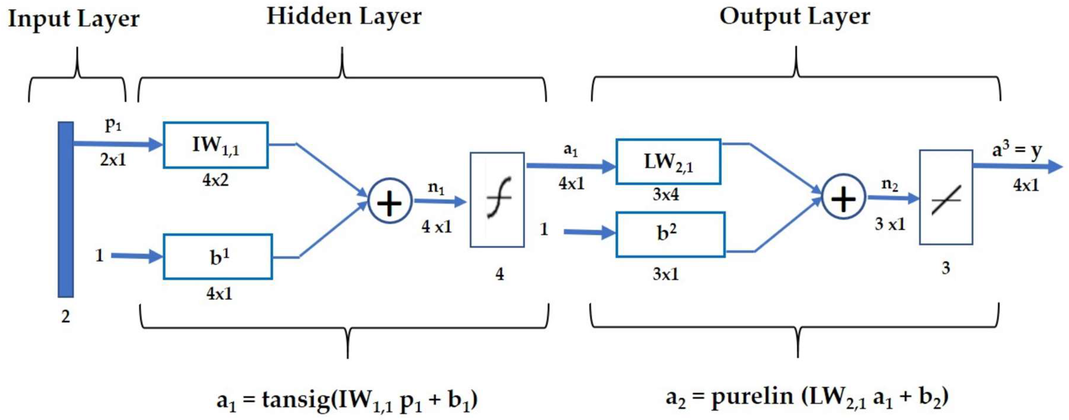
In recent years, neural network technology has been adopted in water quality prediction, in which the back-propagation network is commonly used [26,27]. The model created in this study is a BP neural network model with a single hidden layer (Figure 4). In this ANN, the input layer is R, the hidden layer is a1, the output layer is a2, the weight matrix of the input layer is IW1.1, and the weight matrix from the hidden layer to the output layer is LW2.1. The threshold values of the hidden and output layers are b1 and b2, respectively. f1 and f2 are the neuron transfer functions of the hidden and output layers, respectively.
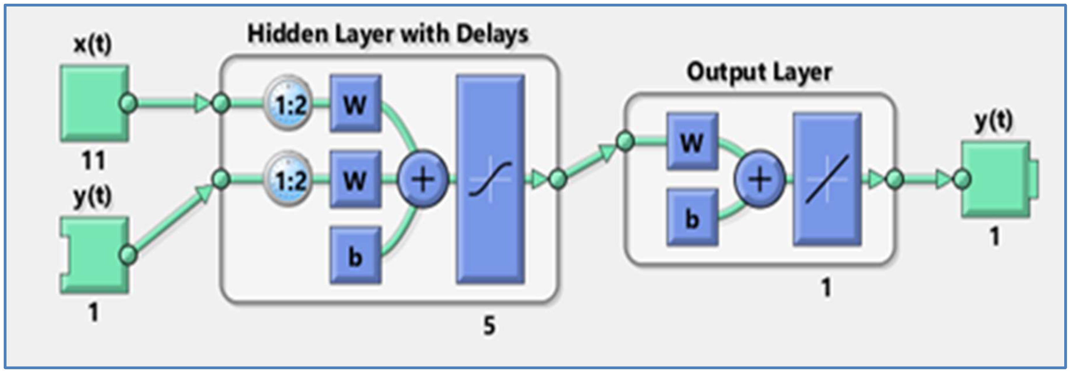
As theoretically verified, the BP model as shown in Figure 4 can handle any nonlinear function with minimum interruptions at any accuracy as long as there are a sufficient number of neurons in the hidden layer of the model and the number of neurons are determined based on a priori and domain knowledge [28]. The proposed ANN model (Figure 5) has two hidden layers of sigmoid neurons that are followed by an output layer of linear neurons. Sigmoid neuron makes the output smoother, and a small change in the input only causes a little variation in the output [29]. This network system can be utilized as a general function approximator. It can estimate any function with a finite number of discontinuities given sufficient neurons in the hidden layer [30,31].
In the developed model structure (Figure 5), the input and output variables are established for the evaluation of water quality. Multiple layers of neurons of the developed ANN structure with nonlinear transfer functions let the network assess nonlinear and linear relationships that underlay input and output vectors. The final output layer is linear, allowing the network to produce values outside the range −1 to +1.
2.5.1. ANN Parameter Selection: Hidden Layers and Nodes
The number of hidden layers in ANN model is usually determined by trial and error. The number of training set samples should be higher than the number of synaptic weights, a rule of thumb for defining the number of hidden nodes [31,32]. Most ANN modelers usually consider a one-hidden-layer network (i.e., the number of hidden nodes is between input nodes and (2*(input nodes) + 1) [30]). However, hidden nodes should not be less than the maximum of one third of input nodes and the number of output nodes. The optimum value of hidden nodes is fixed by trial and error. Networks with minimum number of hidden nodes are usually preferred due to better generalization capabilities and fewer overfitting problems. For this study, a trial and error procedure for the number of hidden node selection was carried out by gradually changing the number of hidden layer nodes.
2.5.2. ANN Parameter Selection: Learning Rate and Momentum
The functions of the learning rate and momentum parameters are to enhance model training and ensure that error is reduced. There is no precise rule for the selection of values for these parameters. Here, the learning rate was controlled by internal validation: after the end of each epoch, the weights were updated. The number of epochs with the smallest internal validation error indicates which weights to select [33]. In this study, the learning rate for the weights connecting input layer and the hidden layer was set at double the size of the learning rate for the weights connecting the hidden layer to the output layer, to increase the rate of network convergence. The momentum was initially fixed at a value of 0.015, with the number of hidden nodes initially estimated as number of input nodes +1, similar to the study conducted by Maier and Dandy (1996) [34].
2.5.3. ANN Parameter Selection: Initial Weights
When the weights of a network is trained by BP, it is always better to initialize from small, non-zero random values, although ANN modelers can start over with a different set of initial weights [22,23]. In this study, the amplitude of a connection between two nodes (synaptic weights) of the proposed ANN networks was adjusted using the normally distributed random numbers having the range from −1 to 1.
2.5.4. ANN Parameter Selection: Selection of Input Variables
In an ANN, one of the main tasks is to determine the model input variables that significantly affect the output variable(s). The selection of input variables is usually related to a priori knowledge of output variables, inspections of time series plots, and statistical analysis of potential inputs and outputs. In this study, the input variables for the present neural network modeling were selected based on a statistical correlation analysis of the runoff quality data, the prediction accuracy of water quality variables, and domain knowledge. Domain knowledge is the specific field knowledge that supports interpretation of data when applying machine learning algorithms like regression, stepwise approach, and classification to predict some test data [35]. In a stepwise approach, separate networks are trained for each input variable [36]. We experimented with the water quality variables included in the parameters listed above in several models to both identify the optimal predictive model and reduce the monitoring cost by including fewer input parameters. After selecting the appropriate input variables, the next step involved determining appropriate lags for each of these variables. The selected appropriate input variables are rainfall amount, duration of rainfall, intensity, runoff coefficient, runoff depth, peak discharge, turbidity, total suspended solids (TSS), dissolved organic carbon (DOC), sodium, chloride, and total nitrate concentrations that were used to develop the ANN model. Appropriate lags are needed for complex problems, where the numbers of potential inputs are significant, and no a priori knowledge is available. Lags allow the model to establish significant connection or bonding between the output and the input variables. By doing so, the best network performance is retained, and the effect of adding each of the remaining inputs in turn is assessed. The correlations between the input variables and output variables are computed separately for each lagged input variable [37]. In this study, optimal networks for each of these combinations were obtained with these time-lagged variables, and the results were compared with the target dataset.
2.5.5. ANN Parameter Selection: Data Partition
It is essential to divide the data set in such a way that both training and overfitting test data sets are statistically comparable. The test set should be approximately 10–30% of the size of the training set of data [38]. In this study, the water quality data were divided into three partitions: the first set contained 70% of the records used as a training set, the second test contained 15% of the records and was used as an overfitting test set, and the rest of the data (15%) were used as the validation set. This process is necessary, because the efficiency of the developed neural network model is highly dependent on the quantity and quality of the data as stated by Palani et al., 2008 [18].
2.5.6. ANN Parameter Selection: Model Performance Evaluation
The model’s efficiency was evaluated using the root mean square error (RMSE, see Equation (7)), the mean absolute error (MAE, see Equation (8)), and R2 (see Equation (9)) [39]. Scatter plots and time series plots were used for visual comparison of the observed and predicted chloride concentrations values.
R2 values of zero indicate that the observed mean is as good a predictor as the model, R2 value of one represents a perfect fit, and a negative R2 value reflects a better predictor than the model [40]. Depending on the sensitivity of water quality parameters and any mismatch between the forecasted and measured water quality variables, one can decide whether the predictive power of the ANN model is accurate enough to inform crucial decisions regarding data usage.
F and F0 could be described using following two equations.
where N is the total number of observations.
The other primary criterion used to select the optimum ANN model was the sum of square error (SSE), determined from the following empirical equation:
where wi are the weights and yi and ŷi are the observed response value and the fitted response value, respectively.
The weights determine how much each response value influences the final parameter estimates. A high-quality data point influences the fit more than a low-quality data point. Weighting data is recommended if the absolute weights are known, or if there is good cause for weighting data differently.
3. Results and Discussion
3.1. Model Output
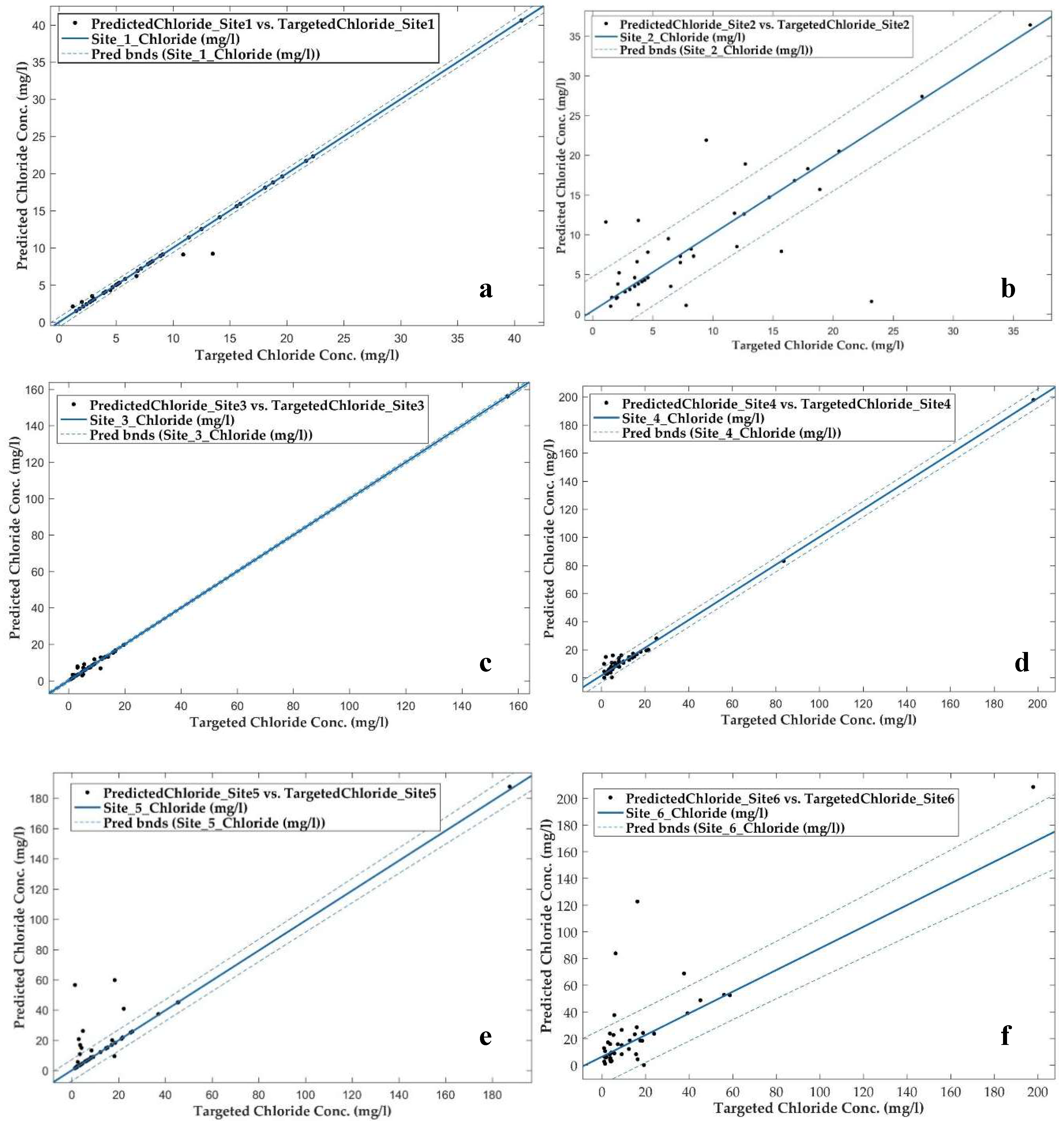
The BP ANN architecture was applied to five hidden layers with different activation functions and initial weights of 0.3, optimum learning rate (0.1), and momentum (0.015), as described in Section 2.5.2 and Section 2.5.3. The proposed ANN model was designed considering 11 input variables from 42 storm events. The sensitivities of the input parameters for the chloride concentration prediction are smaller than those used for the validation dataset. An individual ANN model was run for each of the sites considering the same ANN model structure shown in Figure 5 and the input parameters. The parameters that produce the ‘‘best results” for all sites (Table 1) were then used as the final chloride concentration prediction. The model output or the performance of the ANN model was evaluated based on the R2 values for training, validation, and testing. R2 values for each of the sites were similar for the three data partitions, as indicated in Table 1. The weights are methodically changed by the learning algorithms such that for a given input, the difference between the ANN output, and the actual output was small. The developed ANN model with nine hidden nodes was considered optimal here, considering the output (Table 1 and Table 2). The optimum network parameters associated with the model output are presented in Table 1 and Table 2. Validation errors were calculated after the optimization of the network parameters and the topology. Error was calculated in two ways. First, the cross validation was applied. In this method, data were separated into three parts: training (70%), validation (15%), and testing (15%). The output of the first technique is shown in Table 1. Secondly, the ANN predicted outputs were validated using curve fitting technique. Curve fitting analysis showed a good fit between the targeted or observed and the predicted value (Figure 6). The model outputs were considered acceptable based on the R2 values for training, validation, and testing. In general, the accuracy of the model can be improved by adding data to the validation step or to input variables.
3.2. Curve Fitting Analysis
Curve fitting analysis examines the relationship between target output and the model output. The fit between the target and predicted values were represented for all six sites (Figure 6). Except for site number 1, all the other sites had the best fitting between the two datasets (target and model output). This fulfilled the aims of applying the polynomial bi-square fitting for the presence of concentrated chloride. Polynomial fitting with a high-order polynomial uses the large predictor values as the basis for a matrix, which often creates scaling problems [25]. In this study, most of the analyzed chloride concentration range is from 1 to 20 mg/L, but during the winter these ranges are from 25 to 200 mg/L. No axis range modifications were made here; axes ranges were kept as appropriate for the chloride concentration range. A reasonably good match between the output from the developed ANN model and the curve fitting output was obtained for the sites. To illustrate this, a prediction boundary is provided in Figure 6 for every site with a 95% confidence interval.
Curve-fitting information regarding the developed ANN model output is presented in Table 2; note the SSE, R-Square, and RMSE values are robust. All the ANN models constructed using nine nodes in the hidden layer produced the lowest SSE. Therefore, the site 3 ANN model showed the lowest value of SSE, and the model for Site 6 showed the highest SEE value having the lowest R-square value. In summary, all the ANN models developed here for six sites showed an acceptable range for all the model justification factors. The predicted values are reasonable for all the sites. Curve fitting assessment is a cross-validation approach, proving the accuracy of the developed ANN model. No significant difference in the R2 values can be seen in the Table 2.
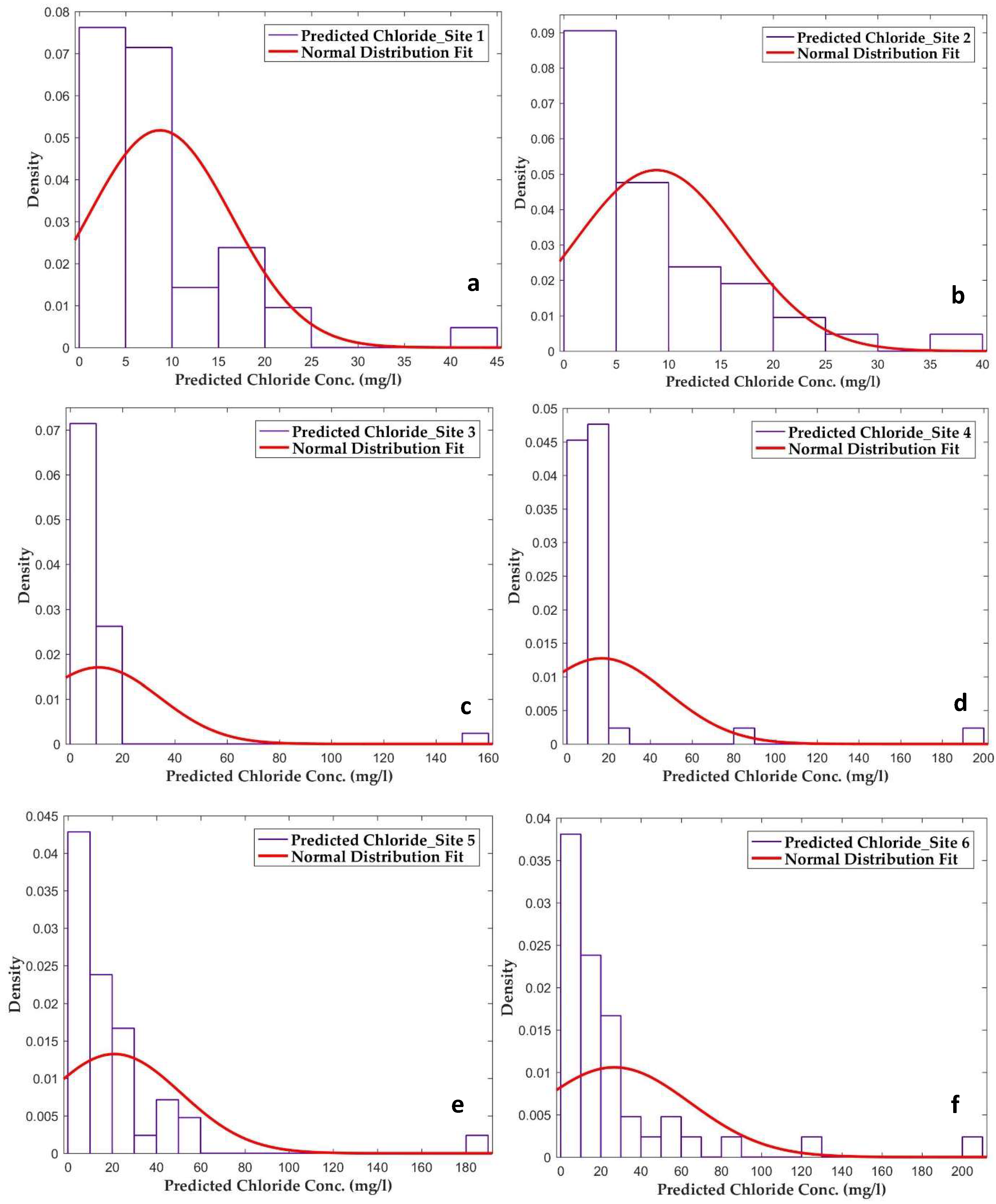
3.3. Density Distribution of the Predicted Chloride Concentration
The density distribution was applied to show the spatial distribution of the predicted chloride concentration values (Figure 7). Usually, the continuous data values tend to cluster around the mean in a normal distribution, and the farther a value is from the mean, the more uncertain it is. The tails are asymptotic, which implies that they approach but never meet the X-axis. In this study, density distribution curve fitting resulted in a 95% confidence interval. This 95% confidence interval means that 95% of values fall within two standard deviations from the mean.
Considering the six study sites, four sites are close to an agricultural field and two are close to a parking lot; the spatial distribution range of the agricultural field sites is smaller than those close to the parking lot. For sites 5 and 6, more than 70% of predicted chloride concentrations are clustered at the mean value, and the peak is wide. On the other hand, the density distribution for sites 1, 2, 3, and 4 cover less than 50% predicted chloride concentration values. Sites 5 and 6 have higher chloride concentrations, because they received salt/chloride from both sides (from the road and the parking lot). The highest spatial range was observed for sites 5 and 6. These results are consistent with the fact that sites 5 and 6 received the chloride from both sides.
3.4. Cross Validation Based on Snow and Precipitation Events
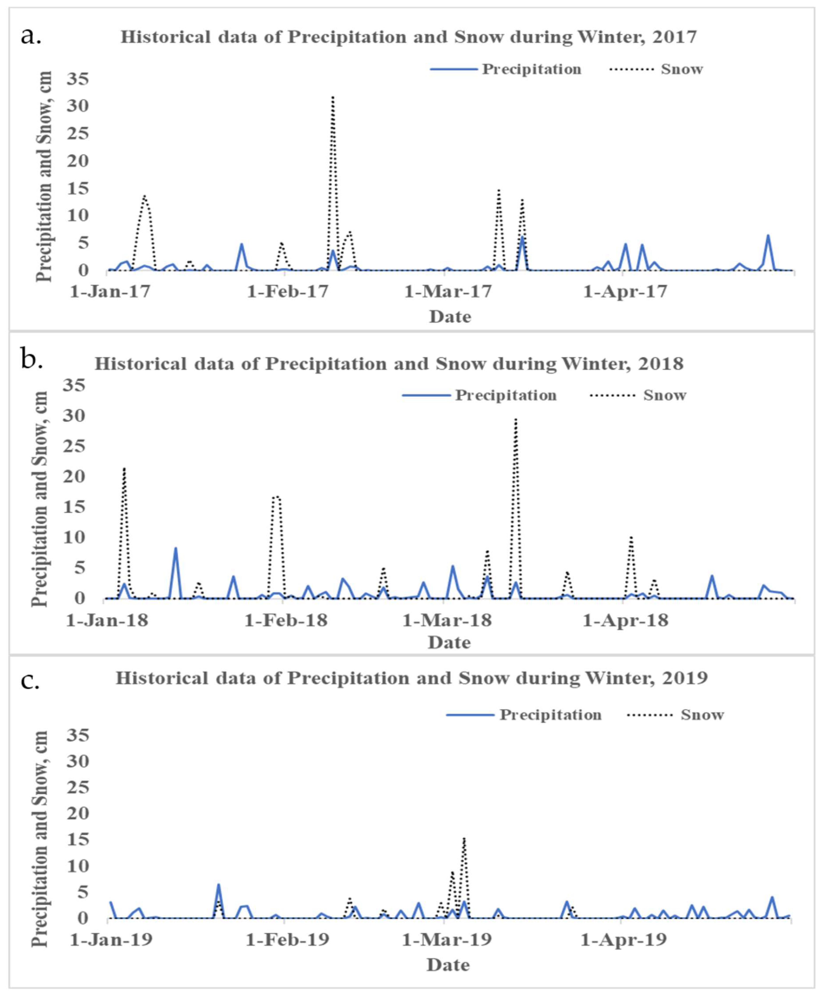
Predicted data were cross validated by taking advantage of temporally close snow and precipitation events. Chloride concentrations were high in storm events that followed severe snow events. Here, we analyzed data from US climate data repositories with three years (2017, 2018, and 2019) of snow and daily precipitation [41] (Figure 8). We then used ANN model to predict chloride concentration based on the results obtained for 2018 data (Figure 9).
Rhode Island receives approximately 94 cm of snow every year, but snowfall totals can vary significantly from town to town, even though the state is relatively small and the terrain is flat [42]. Moreover, the number of snow events vary widely from year to year. Both salt and sand are used on roads during snow events. Given additional chloride derived from snow removal deicers, Rhode Island collects a considerable amount of chloride in its surface water and groundwater, and the salts accumulate in the soils and later percolate into the groundwater. The groundwater becomes saltier every year, since chloride is a dissolved phase and cannot be removed naturally from the water [42,43,44]. Seventy percent of the salt applied to roads stays within the region’s watershed [45]. In this study, chloride data for rain events occurring immediately after snow events in 2017, 2018, and 2019 showed that chloride concentrations increased.
Runoff pollutant concentrations also depend on the size and duration of precipitation event. Both longer duration storms and storms of high intensity impact chloride concentrations. Longer period storms and high intensity storms can dilute the pollutant concentration. For example, on 4 January 2018, a 220 mm snow event preceded 830 mm of rainfall on 13 January 2018, in a storm of 4 hours’ duration. Chloride concentrations were highest after the 13 January storm events. On the other hand, a 147 mm snow event occurred on 10 March 2017, followed by 17 March 2017 storm of 7 hours’ duration. The detected chloride concentration from 17 March 2017 storm events were not significant relative to 2018 storm events. In the ANN model predicting chloride concentration, runoff volume and duration of the rainfall are considered as a positive sensitivity parameter. The March 2017 storm pair, which did not lead to elevated chloride, could reveal the counteracting impacts of street density, street width, and location of the street. Furthermore, the accumulated chloride could be attributed primarily to the amount of salt application, which varies from event to event.
Chloride concentrations greater than 600 ppt (1 mg/L = 1 ppt) are considered harmful for freshwater aquatic life and for the groundwater in general [46]. The developed ANN model prediction (Figure 9) and probability density output (Figure 7) indicated that aquatic habitats at sites 4, 5 and 6 are at risk. State planners need to take necessary action regarding the implications of road salting and snow removal.
4. Conclusions
In this study, a new ANN model is developed to predict elevated chloride concentrations due to road salt and deicer applications in a suburban watershed, based on three years of data (2016–2019) collected at six study sites. Study sites are close to agricultural land (Sites 1, 2, 3, and 4) and an impervious parking lot (Sites 5 and 6). Seasonal variation is evident in the three years of collected data. For the ANN model, input variables were derived from the hydrometeorological database, stormwater runoff quality, key network parameters, and network topology. Preliminary ANN models were constructed using a subset of all data (for 42 storm events from 2016 to 2019) where it covered all four seasons (15 winter events, 6 spring events, 7 summer events, and 15 fall events). A series of sensitivity analyses were considered to determine the relative significance of input variables used in the ANN models. Applying the BP algorithm, developed ANN models showed a good fit between observed and predicted data (about 91%). Model accuracy was initially optimized using a cross-validation approach, and the developed model offers an appropriate and time-efficient approach to constraining the target water quality parameter. The curve fitting assessment resulted in a 95% confidence interval, used here as cross validation of ANN outputs, and provided an optimum summary for every site. The predicted ANN outcome could be more significant or could be trained better if the study duration were longer than three years and/or involved more frequent events. This study focused on the winter season because of the amount of road salt applied to the impervious surfaces, generating high concentrations of chloride in runoff water. The presence of chloride in non-winter season data is negligible compared to the winter season, but the detection of chloride could be due to the use of fertilizer in the agricultural zone. According to the best-fit results, chloride in the study area is mostly affected by the rain and snow that occurred during the winter season, and chloride concentration depends on storm duration, intensity, and runoff volume. We propose neural network modeling as an effective tool for water quality parameter prediction. Finally, density distribution analysis revealed the spatial distribution (the amount of clustered data value around the mean) of the chloride concentration. Density distributions showed about 70% of clustered value is detected for Sites 5 and 6, due to the nearby parking lot. The other four sites, which are close to the agricultural zone, cover less than 50%. These findings again point to used road salt as the main agent of chloride delivery to the groundwater. ANN modeling of environmental data has great potential in future work on improved prediction of chloride and other pollutant concentrations, and provides a useful tool for water resource and environmental managers.
Author Contributions
K.J. and S.M.P., conceptualization; K.J., data collection, analysis, and writing the original draft preparation; S.M.P., writing, review, and editing, S.M.P., funding acquisition. Both the authors have read and agreed to the published version of the manuscript.
Funding
The research study is funded by the Rhode Island Department of Transportation, SPR-234-2362, and the University of Rhode Island.
Acknowledgments
Authors would like to show their gratitude to the Rhode Island Department of Transportation (RIDOT) for their financial support. In addition, we also thank Gavino Puggioni and Nisa Khan for their valuable comments and recommendations. We are also thankful to Thomas Boving for site preparation help. English editing assistance was received from Dawn Cardace.
Conflicts of Interest
The authors declare no conflict of interest. The funders had no role in the design of the study; in the collection, analyses, or interpretation of data; in the writing of the manuscript; or in the decision to publish the results.
References
- Li, D.; Wan, J.; Ma, Y.; Wang, Y.; Huang, M.; Chen, Y. Stormwater Runoff Pollutant Loading Distributions and Their Correlation with Rainfall and Catchment Characteristics in a Rapidly Industrialized City. PLoS ONE 2015, 10, e0118776. [Google Scholar] [CrossRef] [PubMed]
- Koleskar, R.K.; Mattson, N.C.; Peterson, K.P.; May, W.N.; Prendergast, K.R.; Pratt, A.K. Increase in wintertime PM2.5 sodium and chloride linked to snowfall and road salt application. Atmos. Environ. 2018, 177, 195–202. [Google Scholar] [CrossRef]
- Dugan, H.A.; Bartlett, S.L.; Burke, S.M.; Doubek, J.P.; Krivak-Tetley, F.E.; Skaff, N.K.; Summers, J.C.; Farrell, K.J.; McCullough, I.M.; Morales-Williams, A.M.; et al. Salting our freshwater lakes. Proc. Natl. Acad. Sci. USA 2017, 114, 4453–4458. [Google Scholar] [CrossRef] [PubMed] [Green Version]
- Jackson, R.B.; Jobbagy, E.G. From icy roads to salty streams. Proc. Natl. Acad. Sci. USA 2005, 102, 14487–14488. [Google Scholar] [CrossRef] [Green Version]
- Kelting, D.L.; Laxson, C.L.; Yerger, E.C. Regional analysis of the effect of paved roads on sodium and chloride in lakes. Water Res. 2012, 46, 2749–2758. [Google Scholar] [CrossRef]
- Findlay, S.E.G.; Kelly, V.R. Emerging indirect and long-term road salt effects on ecosystems. Year Ecol. Conserv. Biol. 2011, 1223, 58–68. [Google Scholar] [CrossRef]
- Levelton Consultants Limited. Guidelines for the Selection of Snow and Ice Control Materials to Mitigate Environmental Impacts; National Cooperative Highway Research Program, American Association of State Highway, and Transportation Officials; Transportation Research Board: Washington, DC, USA, 2008; Volume 577. [Google Scholar]
- USGS. Evaluating Chloride Trends Due to Road-Salt Use and Its Impacts on Water Quality and Aquatic Organisms; USGS: Reston, VA, USA, 2014.
- Salinity Network. FWRMC Salinity Network Workgroup, Watershed Monitoring Section Quick Links. 2019. Available online: https://floridadep.gov/dear/watershed-monitoring-section/content/salinity-network#:~:text=Over%20the%20past%20several%20decades,of%20groundwater%20from%20our%20aquifers (accessed on 10 May 2019).
- Florida Salinity Network Workgroup. Groundwater Level Conditions for the Upper Floridan Aquifer Based on Percentile Ranks Pilot Study for May, 2010. 2015. Available online: http://publicfiles.dep.state.fl.us/DEAR/DEARweb/FWRMC/FWRMC%20Salnet_document_SNWGWLPRIPilotFinal_cv%20ada%203-27-15.pdf (accessed on 30 September 2015).
- Status and Trends Report, SFNRC Technical Series 2012:1, Salinity and Hydrology of Florida Bay, Status and Trends 1990–2009. South Florida Natural Resources Center, Everglades National Park: Homestead, FL, USA. Available online: https://www.nps.gov/ever/learn/nature/upload/SecureSFNRC2012-1LoRes.pdf (accessed on 10 January 2012).
- Kumar, A.; Sharma, M.P. Assessment of water quality of Ganga river stretch near Koteshwar hydropower station, Uttarakhand, India. Int. J. Mech. Prod. Eng. 2015, 3, 82–85. [Google Scholar]
- Juair, H.; Sharifuddin, M.Z. Sensitivity analysis for water quality index (WQI) prediction for Kinta River. World Appl. Sci. J. 2011, 14, 60–65. [Google Scholar]
- Haykin, S. Neural Networks: A Comprehensive Foundation; Prentice Hall: Upper Saddle River, NJ, USA, 1999. [Google Scholar]
- Vasanthi, S.; Kumar, A. Application of artificial neural network techniques for predicting the water quality index in the parakai lake, Tamil Nadu, India. Appl. Ecol. Environ. Res. 2018, 17, 1947–1958. [Google Scholar] [CrossRef]
- Najah, A.; El-Shafie, A.; Karim Amr, O.A. Application of artificial neural networks for water quality prediction. Neural Comput. Appl. 2013, 22, 187–201. [Google Scholar] [CrossRef]
- Rumelhart, D.E.; Hinton, G.E.; Williams, R.J. Learning internal representations by error propagation. In Parallel Distributed Processing; Rumelhart, D.E., McClelland, J.L., Eds.; MIT Press: Cambridge, MA, USA, 1986. [Google Scholar]
- Palani, S.; Liong, S.; Tkalich, P. An ANN application for water quality forecasting. Mar. Pollut. Bull. 2008, 56, 1586–1597. [Google Scholar] [CrossRef] [PubMed]
- Deep Artificial Intelligence, Hidden Layer. Available online: https://deepai.org/machine-learning-glossary-and-terms/hidden-layer-machine-learning (accessed on 20 December 2012).
- Obuchowski, A. Understanding Neural Networks 1: The Concept of Neurons. 2019. Available online: https://becominghuman.ai/understanding-neural-networks-1-the-concept-of-neurons-287be36d40f (accessed on 23 March 2019).
- Sing, K.; Basant, A.; Malik, A.; Jain, G. Artificial neural network modeling of the river water quality—A case study. Ecol. Model. 2008, 220, 888–895. [Google Scholar] [CrossRef]
- Gavindaraju, R.S. Artificial neural network in hydrology, II: Hydrologic application. ASCE task committee application of artificial neural networks in hydrology. J. Hydrol. Eng. 2000, 5, 124–137. [Google Scholar]
- Wang, Q.H. Improvement on BP algorithm in artificial neural network. J. Qinghai Univ. 2004, 22, 82–84. [Google Scholar]
- Kuo, J.T.; Hseih, M.H.; Lung, W.S.; She, N. Using artificial neural network for reservoir eutrophication prediction. Ecol. Model. 2006, 200, 171–177. [Google Scholar] [CrossRef]
- Mathworks. Matlab User’s Guide (for Use with MATLAB); MathWorks, Inc.: Natick, MA, USA, 2001. [Google Scholar]
- Lee, T.L.; Jeng, D.S. Application of artificial neural network for long-term tidal predictions. Ocean Eng. 2002, 29, 1003–1022. [Google Scholar] [CrossRef]
- Moon, S.K.; Woo, N.C.; Lee, K.S. Statistical analysis of hydrographs and water table fluctuation to estimate groundwater recharge. J. Hydrol. 2004, 292, 198–204. [Google Scholar] [CrossRef]
- Wu, Z.S.; Xu, B.; Yokoyama, K. Decentralized parametric damage detection based on neural networks. Comput. Aided Civ. Infrastruct. Eng. 2002, 17, 175–184. [Google Scholar] [CrossRef]
- Kumar, N. Sigmoid Neuron—Building Block of Deep Neural Networks, Towards Data Science. 2019. Available online: https://towardsdatascience.com/sigmoid-neuron-deep-neural-networks-a4cd35b629d7 (accessed on 7 March 2019).
- Xu, B.; Wu, Z.S.; Yokoyama, K. Response time series-based structural parametric assessment approach with neural networks. In Proceedings of the 1st International Conference on Structural Health Monitoring and Intelligent Infrastructure (SHMII-1 2003), Tokyo, Japan, 13–15 November 2003; Swets & Zeitlinger: Lisse, The Netherlands, 2003; pp. 601–609. [Google Scholar]
- Tarassenko, L. A Guide to Neural Computing Applications; Arnold Publishers: London, UK, 1998. [Google Scholar]
- Hechit-Neilsen, R. Kolmogorov’s mapping neural network existence theorem. In Proceedings of the 1st IEEE International joint Conference of Neural Network, San Diego, CA, USA, 23–28 August 1987; Institute of Electrical and Electronics Engineers: New York, NY, USA, 1987. [Google Scholar]
- Tsoukalas, L.H.; Uhrig, R.E. Fuzzy and Neural Approaches in Engineering; Wiley Interscience: New York, NY, USA, 1997; 587p. [Google Scholar]
- Maier, H.R.; Dandy, G.C. The use of artificial neural networks for the prediction of water quality parameters. Water Resour. Res. 1996, 32, 1013–1022. [Google Scholar] [CrossRef]
- Anand, S. Why Domain Knowledge Is Important in Data Science, medium.com. 2019. Available online: https://medium.com/@anand0427/why-domain-knowledge-is-important-in-data-science-anand0427-3002c659c0a5 (accessed on 18 March 2019).
- Yang, X.; Gandomi, A.; Talatahri, S.; Alavi, A.H. Metaheuristics in Water, Geotechnical and Transport Engineering; Zali, M.A., Retnam, A., Eds.; Elevier Inc.: Amsterdam, The Netherlands, 2013; ISBN 978-0-12-398296-4. [Google Scholar]
- Masters, T. Advanced Algorithms for Neural Networks. A C++ Sourcebook; John Wiley and Sons, Inc.: New York, NY, USA, 1993. [Google Scholar]
- Neuroshell 2TM. Neuroshell Tutorial; Ward Systems Group, Inc.: Frederick, MD, USA, 2000. [Google Scholar]
- Nash, J.E.; Sutcliffe, J.V. River flow forecasting through conceptual models; part 1—A discussion of principles. J. Hydrol. 1970, 10, 282–290. [Google Scholar] [CrossRef]
- Wilcox, B.P.; Rawls, W.J.; Brakensiek, D.I.; Wight, J.R. Predicting runoff from rangeland catchment: A comparison of two models. Water Resour. Res. 1990, 26, 2401–2410. [Google Scholar] [CrossRef]
- Rhode Island Division of Planning. Road Salt/Sand Application in Rhode Island, Statewide Planning; Technical Paper Number: # 163; Rhode Island Division of Planning: Providence, RI, USA, 2014. Available online: http://www.planning.ri.gov/documents/LU/RoadSaltTechPaper2013_12114rev.pdf (accessed on 31 March 2014).
- Hinsdale, J. How Road Salt Harms the Environment, State of the Planet. 2018. Available online: https://blogs.ei.columbia.edu/2018/12/11/road-salt-harms-environment/ (accessed on 11 December 2018).
- Elgin, E.; Salt Runoff Can Impair Lakes. Salting Roads, Parking Lots, and Sidewalks Can Turn Our “Fresh” Water Salty. 2018. Available online: https://www.canr.msu.edu/news/salt_runoff_can_impair_lakes (accessed on 22 February 2018).
- Kelting, D.; Laxson, C. Review of Effects and Costs of Roads De-Icing with Recommendations for Winter Road Management in the Adirondack Park. Adirondack Watershed Institute Report # AWI2010-01. 2010. Available online: http://www.protectadks.org/wp-content/uploads/2010/12/Road_Deicing-1.pdf (accessed on 22 February 2010).
- Rastogi, N. Salting the Earth: Does Road Salt Harm the Environment? The Green Lantern. 2010. Available online: https://slate.com/technology/2010/02/does-road-salt-harm-the-environment.html (accessed on 16 February 2010).
- Nagpal, N.K.; Levy, D.A.; MacDonald, D.D. Ambient Water Quality Guidelines for Chloride 2. National Library of Canada Cataloguing in Publication. Environmental Management Act, 1981. (3 of 22). 2004. Available online: http://wlapwww.gov.bc.ca/wat/wq/BCguidelines/chloride.html (accessed on 15 January 2004).
Figure 1.
Chloride concentration trends from 1992 to 2012 in the USA show regional differences (modified from United States Geological Survey Report, 2014).
Figure 1.
Chloride concentration trends from 1992 to 2012 in the USA show regional differences (modified from United States Geological Survey Report, 2014).

Figure 2.
The map illustrates the location of the study area in Rhode Island, USA. Red bounding box shows the exact location of the study site shown above (Google Earth screenshot- on the right).
Figure 2.
The map illustrates the location of the study area in Rhode Island, USA. Red bounding box shows the exact location of the study site shown above (Google Earth screenshot- on the right).

Figure 3.
Variability in observed chloride concentrations in runoff are shown, from 2016 to 2019.

Figure 4.
This diagram illustrates the structure of a conventional feed-forward back-propagation neural network model
Figure 4.
This diagram illustrates the structure of a conventional feed-forward back-propagation neural network model

Figure 5.
This diagram illustrates the structure of the artificial neural network (ANN) model developed in this work.
Figure 5.
This diagram illustrates the structure of the artificial neural network (ANN) model developed in this work.

Figure 6.
Curve fitting assessment between ANN output and target data of six different sites. (a) Site 1, (b) Site 2, (c) Site 3, (d) Site 4, (e) Site 5, and (f) Site 6. Site 1, 3, 4 an 5 showed the similar trend and data were not scattered. On the other hand, site 2 and 6 has scattered data point but 80% of dataset were in the confidence interval.

Figure 7.
Density distributions (ANN outputs) for chloride concentrations at all sites (a) Site 1, (b) Site 2, (c) Site 3, (d) Site 4, (e) Site 5, and (f) Site 6 reveal shifting means. Spatial distribution covered <50% for site 1, 2, 3 and 4 whereas site 5 and 6 covered >70% of predicted chloride.
Figure 7.
Density distributions (ANN outputs) for chloride concentrations at all sites (a) Site 1, (b) Site 2, (c) Site 3, (d) Site 4, (e) Site 5, and (f) Site 6 reveal shifting means. Spatial distribution covered <50% for site 1, 2, 3 and 4 whereas site 5 and 6 covered >70% of predicted chloride.

Figure 8.
Precipitation and snow events (a) 2017, (b) 2018, and (c) 2019 in South Kingstown, RI. (a) total four significant snow events (>10 cm) and low to moderate precipitation events appeared during winter in 2017; (b) three significant snow (>10 cm) events (among them one was the worst >25 cm) and low to moderate with high frequency precipitation occurred during winter in 2018; and (c) only one significant snow and low to moderate precipitation happened during the winter in 2019.

Figure 9.
Predicted concentrations for three sites 4, 5, and 6 reflecting heavy Cl inventory in Winter 2018.
Figure 9.
Predicted concentrations for three sites 4, 5, and 6 reflecting heavy Cl inventory in Winter 2018.


Table 1.
ANN model output for all the sites.
| Location | Performance (Epoch) | Training (%) | Validation (%) | Testing (%) |
|---|---|---|---|---|
| Site_1 | 9 | 95 | 87 | 88 |
| Site_2 | 5 | 100 | 72 | 95 |
| Site_3 | 5 | 100 | 52 | 93 |
| Site_4 | 3 | 99 | 97 | 93 |
| Site_5 | 3 | 99 | 78 | 91 |
| Site_6 | 2 | 97 | 83 | 88 |
Table 2.
Summary of the curve fitting assessment.
| File Name | SSE | R-Square | Adj R-sq | RMSE |
|---|---|---|---|---|
| Site_1 | 1.96 | 0.99 | 0.99 | 0.22 |
| Site_2 | 171.58 | 0.93 | 0.93 | 2.07 |
| Site_3 | 7.9 | 0.99 | 0.99 | 0.44 |
| Site_4 | 231.3 | 0.99 | 0.99 | 2.4 |
| Site_5 | 473.6 | 0.98 | 0.98 | 3.4 |
| Site_6 | 4051 | 0.93 | 0.92 | 10.06 |
Publisher’s Note: MDPI stays neutral with regard to jurisdictional claims in published maps and institutional affiliations. |
© 2020 by the authors. Licensee MDPI, Basel, Switzerland. This article is an open access article distributed under the terms and conditions of the Creative Commons Attribution (CC BY) license (http://creativecommons.org/licenses/by/4.0/).
Share and Cite
MDPI and ACS Style
Jahan, K.; Pradhanang, S.M. Predicting Runoff Chloride Concentrations in Suburban Watersheds Using an Artificial Neural Network (ANN). Hydrology 2020, 7, 80. https://0-doi-org.brum.beds.ac.uk/10.3390/hydrology7040080
AMA Style
Jahan K, Pradhanang SM. Predicting Runoff Chloride Concentrations in Suburban Watersheds Using an Artificial Neural Network (ANN). Hydrology. 2020; 7(4):80. https://0-doi-org.brum.beds.ac.uk/10.3390/hydrology7040080
Chicago/Turabian StyleJahan, Khurshid, and Soni M. Pradhanang. 2020. "Predicting Runoff Chloride Concentrations in Suburban Watersheds Using an Artificial Neural Network (ANN)" Hydrology 7, no. 4: 80. https://0-doi-org.brum.beds.ac.uk/10.3390/hydrology7040080
Note that from the first issue of 2016, this journal uses article numbers instead of page numbers. See further details here.