Article

Analyzing the Impacts of Serial Correlation and Shift on the Streamflow Variability within the Climate Regions of Contiguous United States

1
FTN Associates, Ltd., 3 Innwood Cir # 220, Little Rock, AR 72211, USA
2
School of Civil, Environmental and Infrastructure Engineering, Southern Illinois University, Carbondale, IL 62901, USA
3
Department of Mechanical Engineering and Energy Processes, Southern Illinois University, Carbondale, IL 62901, USA
4
Bayer-Risse Engineering Inc., 78 State Highway 173 W, Suite#6, Hampton, NJ 08827, USA
*
Author to whom correspondence should be addressed.
Submission received: 7 October 2020 / Revised: 16 November 2020 / Accepted: 19 November 2020 / Published: 21 November 2020

Abstract

:
The spatiotemporal hydrologic variability over different regions of the contiguous United States poses the risk of droughts and floods. Understanding the historic variations in streamflow can help in accessing future hydrologic conditions. The current study investigates the historic changes in the streamflow within the climate regions of the continental United States. The streamflow records of 419 unimpaired streamflow stations were grouped into seven climate regions based on the National Climate Assessment, to evaluate the regional changes in both seasonal streamflow and yearly streamflow percentiles. The non-parametric Mann–Kendall test and Pettitt’s test were utilized to evaluate the streamflow variability as a gradual trend and abrupt shift, respectively. The Walker test was performed to test the global significance of the streamflow variability within each climate region based on local trend and shift significance of each streamflow station. The study also evaluated the presence of serial correlation in the streamflow records and its effects on both trend and shift within the climate regions of the contiguous United States for the first time. Maximum variability in terms of both trend and shift was observed for summer as compared to other seasons. Similarly, a greater number of stations showed streamflow variability for 5th and 50th percentile streamflow as compared to 95th and 100th percentile streamflow. It was also observed that serial correlation affected both trends and steps, while accounting for the lag-1 autocorrelation improved shift results. The results indicated that the streamflow variability has more likely occurred as shift as compared to the gradual trend. The outcomes of the current result detailing historic variability may help to envision future changes in streamflow. The current study may favor the water managers in developing future decisions to resolve the issues related to the streamflow variability in flood and drought-prone regions.

1. Introduction

The components of the earth’s environment that are supporting the human civilization, directly and indirectly, are vulnerable to any changes from its natural state. Significant divergence from the normal hydroclimatic conditions poses impacts on society and the environment [1]. The freshwater within hydrosphere is an important component behind the flourishing of human civilization and maintaining the terrestrial biological systems. The increased variability in the hydrologic variability is caused by the varieties of drivers that change the water cycle and hydrologic systems [2,3,4]. Recent studies have also highlighted the changes in hydro-climatology due to the changing climate and global warming. Intergovernmental Panel on Climate Change, IPCC [5] reported that human activities have imposed an approximate rise in global temperature by 1 °C after the pre-industrial age and global warming will stretch to 1.5 °C between 2032 and 2052 if the temperature continues to increase at the current rate. The increase in mean temperature and temperature extremes have substantially changed the components of the water cycle resulting in hydrologic non-stationarity [6,7]. The negative consequences of the hydrologic variability are further amplified by population stress and human interventions [8].
Streamflow is a major hydrologic variable that governs socioeconomic activities. Streamflow largely influences the water supply of the communities and hazards such as floods and droughts. Between 1980 and 2019, floods contributed to 12.5% and droughts contributed to 10.2% of the losses amongst climate disasters exceeding billion dollars of economic damage over the United States [9]. A plethora of studies have documented the hydrologic changes manifested as frequent floods [10,11] and frequent droughts [12,13,14] over the past few decades. The changes in the frequency and intensity of hydrologic events such as precipitation and streamflow can potentially affect the environment and challenge critical engineering infrastructures. Such challenges associated to hydrologic variability have driven water managers to understand the historic variability and predict future hydrology. Furthermore, the hydrologic behavior of the contiguous U.S. is very diverse, based on the regional climate making studies more challenging. Regions of the Western US are semi-arid, desert, oceanic or Mediterranean while humid Eastern US is both continental and subtropical. Consequently, quantifying the streamflow variabilities across the climate regions of the contiguous United States can help water managers in making future decisions for a sustainable and safer future.
Streamflow variability can be attributed to its own natural variability, climate change, and human interventions like diversion, water banking, and changes in land use. Significant studies have utilized unimpaired streamflow stations to evaluate the changes in the streamflow solely caused by factors like natural variability and climate change minimizing the effects of human interventions [15,16]. Studies have utilized hydroclimatic teleconnection to forecast the streamflow [17,18] while understanding the historic variability in the streamflow can recognize future changes and improve forecasting skills as well. The historic variability in the streamflow can be assessed as trend or shift. Trends are gradual and are often observed throughout the length of the historic records while non-homogeneity in the data also termed as shift is the abrupt historic changes representing a sudden change in the climate system. Studies have significantly focused on the trends while evaluating the temporal variability in the historic data but there is a lack of attention towards the shift in the data [19]. Previously, Kerr [20] has documented a sudden shift in the Norther Pacific Climate during the period 1976–1977, which gradually affected the sea surface temperatures of other regions of the Pacific Ocean. These changes later became popular as the regime shift in the climate system and were observed in multiple hydroclimatic variables [21,22]. Villarini et al. [22] indicated that shift should be evaluated before analyzing the trend. There should be a clear distinction among trend and shift to attribute whether the variability is caused by long term variability and/or the variability is caused by abrupt shift [23]. Thus, it is important to test the presence of shift in the streamflow records while estimating the historic trend.
In 1976 linear regression was utilized to access the trend in precipitation for West Africa [24]. Since then both non-parametric and parametric approaches to evaluate the temporal variability of hydrologic records have been documented [11,15,23,25,26,27,28]. The non-parametric approach is more suitable compared to the parametric method as it does not assume any distribution in the time series and can easily account for extremes and outliers. The Mann–Kendal (MK) test is a widely used non-parametric method used to evaluate the trend in hydroclimatic records which was derived by Kendall [29] and Mann [30]. Furthermore, significant studies have been performed to modify the MK test to improve the results [23,26,31]. Multiple techniques have evolved for shift estimation in any time series data. The Von Neumann ratio test evaluates the shift; however, it cannot evaluate the location of the shift in the data [32]. The standard normal homogeneity test is sensitive to evaluate the shift towards the end of the time-series [33]. Pettitt’s test is a non-parametric test that does not assume any distribution in the time series, and it can equally detect the location of the shift in the middle of the time series [34,35].
The hydroclimatic data usually show serial correlation signifying the physical processes of different frequencies. Previously, Yue et al. [31] have documented the trend overestimation in the presence of positive autocorrelation in the time series. The presence of more than one significant autocorrelation results in long term persistence (LTP) and was identified by Hurst [36] and is also known as the Hurst phenomenon. LTPs are significantly observed in hydroclimatic and geophysical records [37] and should be removed from the time series while evaluating the true variability of the time-series. Both Pettitt and MK are documented in previous studies and have the same theoretical base while the Pettitt test has received less attention compared to the MK test [19,23]. The effectiveness of the MK test was studied earlier by Yue and Pilon [38] while a similar study for the shift was not performed until 2015 by Mallakpour and Villarini [11]. Similarly, Yue et al. [31] suggested removing the autocorrelation in the time-series while estimating the trend but a similar study for the shift was not performed until 2016 when Serinaldi and Kilsby [19] pre-whitened the series before performing the Pettitt test. Based on the documented literature, studies have not accounted for the serial correlation while evaluating the shift in the streamflow across the contiguous United States.
The primary objective of the current research was to evaluate the streamflow variability over six geographic regions with different climatic conditions within the contiguous US defined by the National Climate Assessment (NCA). Previous studies have established the presence of serial correlation and shift in the streamflow records [16,23,26,31]. The current study utilized a holistic approach to evaluate the streamflow variability considering both non-homogeneity and serial correlation while evaluating the trend. The study also evaluated the effects of serial correlation during shift estimation within the climate regions of the contiguous United States which is novel to the existing literature. The current study answers the following research queries: (1) What is the overall streamflow variability within the climate regions of the contiguous US? (2) What is the significance of the serial correlations and do they affect the significance of both trend and shift? (3) What is the effect of both serial correlation and shift on the historic streamflow trend? To address the aforementioned questions following measures were adopted: (1) different versions of the MK test were performed considering serial correlation to avoid error in the estimates of trend significance; (2) a Thiel–Sen approach was utilized to estimate the trend magnitude; (3) Pettitt’s Test was utilized to evaluate the significance of the shift after de-trending the time series to consider the serial correlation; and (4) the MK test was applied again before and after the evaluated change point (shift) to distinguish between the gradual change and regime shift.

2. Materials and Methods

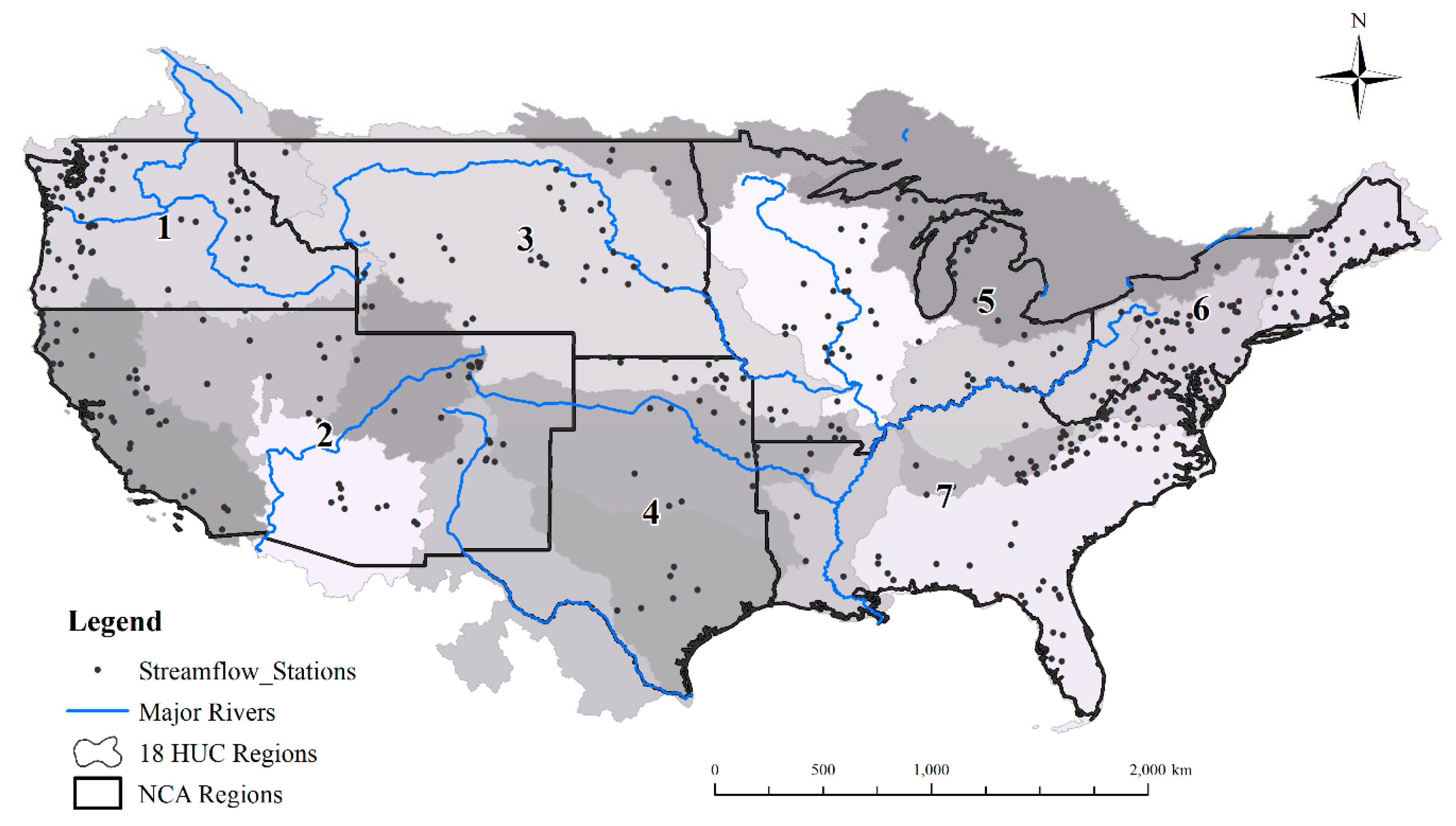
2.1. Study Area and Data

The study was performed within climate regions as suggested by the NCA (https://nca2014.globalchange.gov/) [39] but the Great plains were divided into Northern and Southern Great plains. Great plains were divided into two smaller regions to consider the variations in hydroclimatology along the north–south stretch similar to the references [40,41]. Altogether seven regions accounted for in the study were Northwest (NW), Southwest (SW), Northern Great Plains (NGP), Southern Great Plains (SGP), Midwest (MW), Southwest (SW), and Northeast (NE) as shown in Figure 1. NW and SW are highly influenced by the jet streams and winds from the Pacific Ocean, the streamflow in these regions are snow fed mostly contributed by the winter precipitation. The regions of the eastern US contributed by NGP, SGP, SE, MW, and NE are mostly influenced by the subtropical storms arising from the Atlantic Ocean. Along with the NCA regions, the 18 Hydrologic Units and major rivers in the continental US are also presented in Figure 1. Readers are referred to reference [39] for more details on the climate of the aforementioned climate regions.
The Hydro-Climate Data Network 2009 (HCDN-2009) maintained by the United States Geological Survey (USGS) provides the unimpaired streamflow dataset for 743 streamflow stations throughout the United States [42]. The corresponding unimpaired streamflow stations are upstream of any human intervention. Streamflow stations in each region were selected based on the temporal continuity and spatial distribution of the data. The spatial distribution of the selected streamflow stations is shown in Figure 1. A total of 419 out of 743 stations were selected with 50 to 60 years of continuous data. The streamflow data corresponding to NCA Region are presented in Table 1. The mean monthly streamflow data and daily data were obtained from the USGS website (http://www.usgs.gov/). The daily data were utilized to evaluate the yearly median and percentiles (5th percentile, 50th percentile, 95th percentile, and 100th percentile) to analyze the overall variability in the streamflow data. Similarly, four seasonal streamflow volumes were calculated from mean monthly streamflow and analyzed for the historic variability. The four seasonal streamflow volumes corresponding to winter (January–March), spring (April–June), summer (July–September), and autumn (October–December). Eventually, the streamflow stations of the contiguous US were grouped altogether into seven climate regions to perform regional analysis.

2.2. Methodology

This section first presents the calculation of trend, followed by the calculation of shift and finally calculating the trend before and after the change points.

2.2.1. Calculation of Trend

Three varieties of the MK tests were used to analyze the trend in the streamflow. First, the MK test without autocorrelation was used and represented henceforth as MK1. Second, the MK test considering lag-1 autocorrelation (MK2) and trend pre-whitening was used [31]. Third, the MK test considering LTP (MK3) as proposed by Hameed [26] was used. After performing the MK tests, the Pettitt test was utilized to evaluate the shift. While performing shift analysis, serial correlation was considered and MK tests were performed again before and after the change points. The tests are explained below. Readers are referred to Mann [30] and Kendall [29] for details on the MK1 test. Similarly, details on trend free pre-whitening and MK2 test can be obtained from [31] and details on Hurst significance and MK3 trends can be obtained from Hameed [26]. The magnitude of the trend was obtained using the Thiel–Sen Slope [43,44].

2.2.2. Calculation of Shift

The shift in the streamflow data of the contiguous US was evaluated with the help of the Pettitt test [34]. For a set of random variables, {X1, X2, … XT} is said to have a change point (location of shift) τ, if Xt for t < τ has different distribution as compared to the distribution of Xt for t > τ. The null hypothesis H0 was assumed as there was no shift in the data, thus τ should be equal to T. The alternate hypothesis H1 is 1 ≤ τ ≤ T. The test was based on the following statistics.
K T = | U t , T | 1 τ T m a x
where,
U t , T = i = 1 t j = i + 1 T S i g n ( X j X i )
Sign is the same function as in the MK test. The statistic Ut,T is similar to the Mann–Whitney statistic. To account for the serial correlation as described earlier, the MK2 test was utilized for pre-whitening the time series [31]. The ordinary shift estimates before accounting for lag-1 autocorrelation is referred as Shift-1. The change point and the shift were evaluated again with the pre-whitened time series. Shift after accounting lag-1 autocorrelation and considering the trend free pre-whitening (removing lag-1 autocorrelation) is referred hereafter as Shift-2.

2.2.3. Calculation of Field Significance

In addition to the analysis of the trend and shift, field significance was evaluated utilizing the Walker test [45]. Field significance should be assessed while evaluating the regional variability to test whether the evaluated variability like trend and shift are globally significant or if the trend and shift are evaluated by chance. The Walker test resulted in the global significance of the trend and shift based on the p-values of the local trend and shift in each climate region. The Walker test was utilized to access the global significance of both seasonal and percentile variability (gradual and abrupt) at the statistical significance of p ≤ 0.10.

3. Results and Discussions
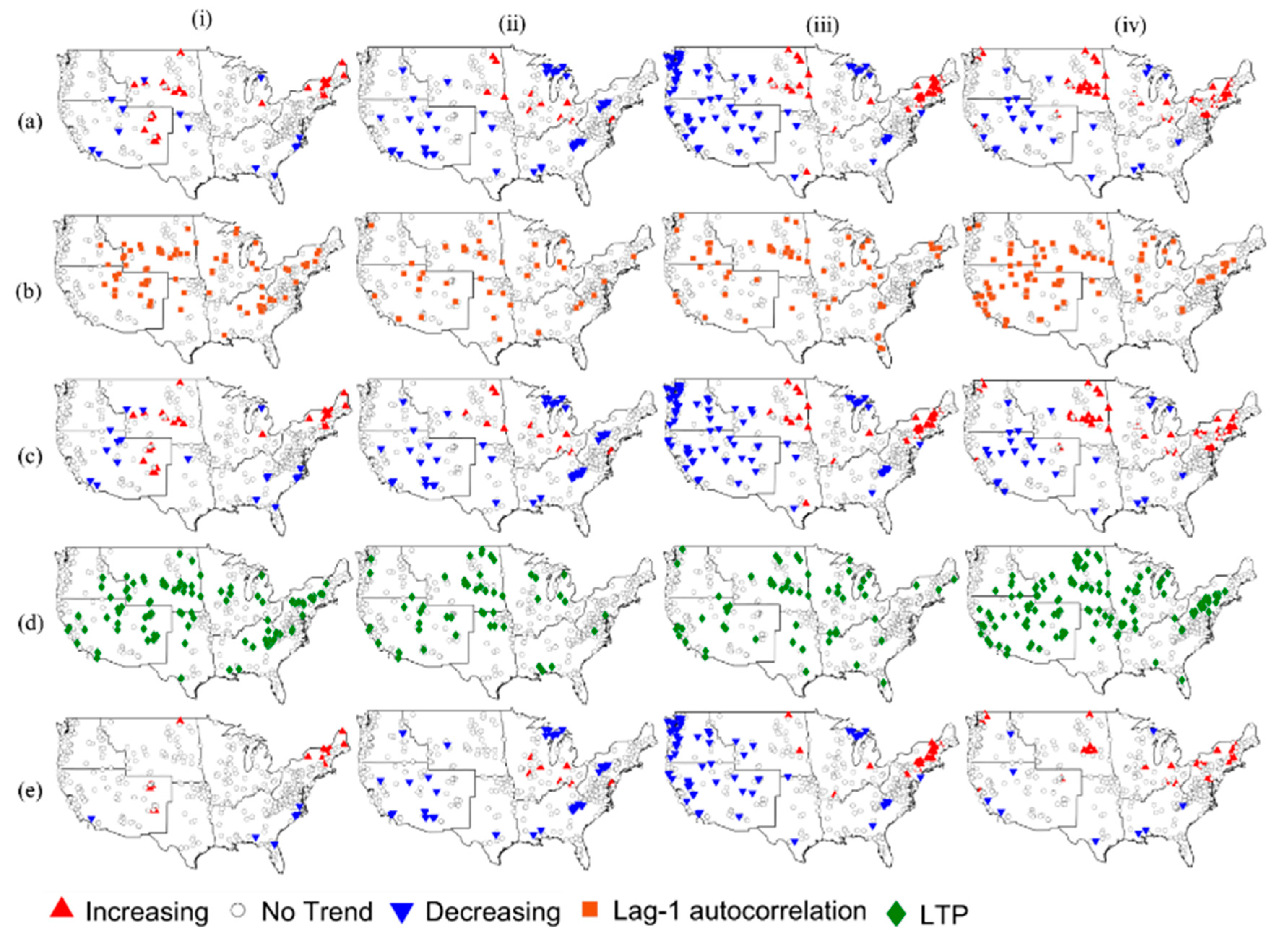
First, the MK1 trend and Pettitt shift test was evaluated for the yearly spring–summer streamflow of 419 stations within the contiguous US. Spring–summer streamflow was analyzed to evaluate the temporal variability of yearly streamflow because spring–summer streamflow contributes to the major portion of yearly streamflow [46,47]. The assessment of spring-summer streamflow is also important because they highly govern the recharge of groundwater, soil moisture, and evapotranspiration impacting the forest and agriculture [17,48]. Out of 419 streamflow stations, 14/38 stations showed an increasing/decreasing MK1 trend and 18/44 stations showed increasing/decreasing shifts. Regions showing (increasing/decreasing) trend at the statistical significance of p ≤ 0.1 were NW (0/2), SW (0/15), NGP (6/1), SGP (0/4), MW (8/8), and SE (0/8). Similarly, regions showing (increasing/decreasing) shift at the statistical significance of p ≤ 0.1 were NW (0/2), SW (0/15), NGP (10/6), SGP (0/3), MW (7/8), SE (0/11), and NE (1/1).
Overall, it was observed that very few stations showed trend and shift for spring–summer streamflow. Some stations of NGP and MW showed both increasing trend and shift while the rest of the stations showed a decreasing trend and shift in spring–summer streamflow volume. Each season is anticipated to show different hydrologic variability resulting from the differences in effects of hydroclimatic variables like precipitation and temperature during each season. For example, it is documented that due to early snowmelt caused by the rise in temperature, the summer streamflow in the western US has declined unlike spring streamflow [49]. Winter snowpack melts during spring and summer drive a major portion of the streamflow during these seasons (spring and summer) in NW and SW while early snowmelt moves the streamflow peaks towards early spring causing an increase in spring streamflow and decrease in summer streamflow. In such cases, although a station has seasonal variability they cancel and do not show up while evaluating yearly or here spring–summer variability. This motivated us to evaluate the variability in the streamflow for each season separately. Similarly, percentile streamflow was also evaluated to elucidate the temporal variability of the streamflow distribution.
For a detailed study, yearly low flow (5th percentile yearly streamflow—Q05), high flows (95th and 100th percentile yearly streamflow—Q95 and Q100), and yearly median streamflow (Q50) metrics along with four seasonal streamflow volume were analyzed to evaluate the overall variability in the streamflow distribution. The results for the trend and shift of the aforementioned streamflow metrics are presented in the two ensuing sections. Trends in seasonal and percentile streamflow records are presented in the first section. Similarly, shift evaluation and trend before and after the change points for both seasonal and percentile streamflow are presented in the second section.

3.1. Trend Results

3.1.1. Trend in Seasonal Streamflow

All the results corresponding to MK1, MK2, and MK3 are at the statistical significance of p ≤ 0.05. The test for lag-1 autocorrelation and LTP were performed at the statistical significance of p ≤ 0.1 allowing the consideration of serial correlation in a greater number of stations subsiding the error in trend estimation. The results for serial correlation and trend in (i) winter, (ii) spring, (iii) summer, and (iv) autumn streamflow volume for all climate regions within the contiguous US are presented in Figure 2. Row (a), (c), and (e) of Figure 2 show the stations showing significant trends based on the MK1, MK2, and MK3 tests, respectively, for the seasonal streamflow. The upward/downward triangles represent the stations showing increasing/decreasing trends. In Figure 2b orange square markers represent the stations showing lag-1 autocorrelation. Similarly, green diamond markers in Figure 2d show the spatial location of stations showing LTP for respective seasonal streamflow volume.
A higher number of stations showed MK1, MK2, and MK3 trends for the summer followed by spring and autumn while a smaller number of stations showed trend during the winter season. Further, both lag-1 autocorrelation and LTP were detected in all climate regions. A higher number of stations showed lag-1 autocorrelation and LTP during autumn and winter as compared to spring and summer. The spatial distribution of stations with lag-1 autocorrelation and LTP as shown in Figure 2b,d, respectively, varied with both region and season. The number of stations within each climate region showing significant MK1, MK2, and MK3 trends during each season is summarized in Table 2. Lag-1 autocorrelation did not affect the significance of the trend; thus, MK1 and MK2 yielded similar results as shown in Table 2. The current study performed a regional analysis to evaluate the streamflow variability within the climate regions of the contiguous United States. Thus, the walker test was performed to evaluate whether the evaluated variability within each region was by chance or whether the evaluated variability was field significant based on the local significance of the trend and shift for each station. Table 2 shows the regions which are field significant at p ≤ 0.1 with bold entries. The result strongly indicates that the temporal variation of streamflow within the climate regions of the contiguous US varied with season. In other words, the results indicated that a trend in streamflow depends upon the climate and topography represented by the climate regions. All but the SE region were field significant for MK1, MK2, and/or MK3 test and the trend results of NW were not field significant during spring.
Within NE out of 65 stations, 22, 20, and 20 stations showed positive MK1, MK2, and MK3 trends, respectively, during summer which was field significant. Previously, Sagarika et al. [16] considering USGS hydrological regions have also documented the increase in streamflow at a similar location represented by New England. In addition to NE, some stations of NGP and MW also showed an increasing seasonal trend which may be attributed to increased precipitation [50,51,52]. Few stations of NGP showed an increasing trend during all seasons as shown in Figure 2 and Table 2, with all MK1 and MK2 results being field significant. Within NGP, 10 and 9 stations showed positive MK1 and MK2 trend, respectively, during summer and, similarly, 15 and 14 stations showed positive MK1 and MK2 trend, respectively, during autumn. Very few stations of MW also showed a positive trend during all seasons which was field significant. Stations of MW showed field significant positive trend during winter with 11 stations showing an MK1 and 9 stations showing an MK2 trend. Overall, it was observed that a greater number of streamflow stations of western US (NW and SW) showed a negative trend during summer. Out of 56 stations of NW, 26/27 stations showed a negative MK1/MK2 trend during summer which was field significant. Furthermore, 25 stations within NW also showed a negative MK3 trend during summer which was not field significant. Out of 76 stations of SW, 26, 25, and 22 stations showed negative MK1, MK2, MK3 trends, respectively, during summer which was field significant. A comparatively smaller number of stations within SW showed a negative trend during spring. Streamflow are mostly controlled by climate, physiography, and human interventions [53]. Snow dominant regions with colder climates are more vulnerable to rises in temperature and showed different variability in streamflow as compared to rainfall dominant regions. Most of the stations of snow dominant western US (NW and SW) during summer showed a decreasing trend as compared to other seasons reflecting drier conditions. This can be attributed to the increase in temperature inducing reduced and early snowmelt in the western US, further changing the timing of the peak streamflow of snow-fed watersheds from summer towards early spring.
Figure 3 shows the changes in the streamflow during the study period (60 years for NE and 50 years for the rest of the regions) as the percent change of the mean streamflow of the corresponding station. The changes in streamflow magnitude shown in Figure 3 were calculated based on the Thiel–Sen slope calculated for the stations showing an MK1 trend at 95% significance. Statistical correlation within a time series can conceal the actual variability, misleading the estimation of trend [31,54,55]. MK2 results were similar to MK1 results, which signifies that lag-1 autocorrelation does not account for entire serial correlation in the streamflow within the contiguous United States. A smaller number of stations showed an MK3 trend as compared to MK1 and MK2 tests supporting the significant effect of LTP while detecting the trend significance. A smaller number of stations in NW showed LTP and a smaller number of stations in SGP showed lag-1 autocorrelation as compared to other climate regions. LTPs are common in hydroclimatic and geophysical records [37] and should be evaluated while attributing the trends. LTPs account for the low-frequency processes such as volcanic and solar activities while the trend after removing LTP (MK3) signifies the changes in the time series caused by factors like anthropogenic activities and climate change. It was observed that a greater number of stations showed MK3 trend during summer, attributing to the higher temperature during the season caused by changing climate. Most of the stations in NW and SW showed a decreasing MK3 trend during the summer season indicating the decline in streamflow which cannot be attributed to the long-term variability. These changes may be attributed to the recent changes snowmelt—mentioned earlier and changes in other hydroclimatic variables such as precipitation and temperature resulting from climate change. Similarly, stations of NE showed increasing MK3 trend during winter, summer, and autumn which may be attributed to the rise in temperature and moisture holding capacity of the storms traveling NE region through the Atlantic Ocean and the Gulf of Mexico.

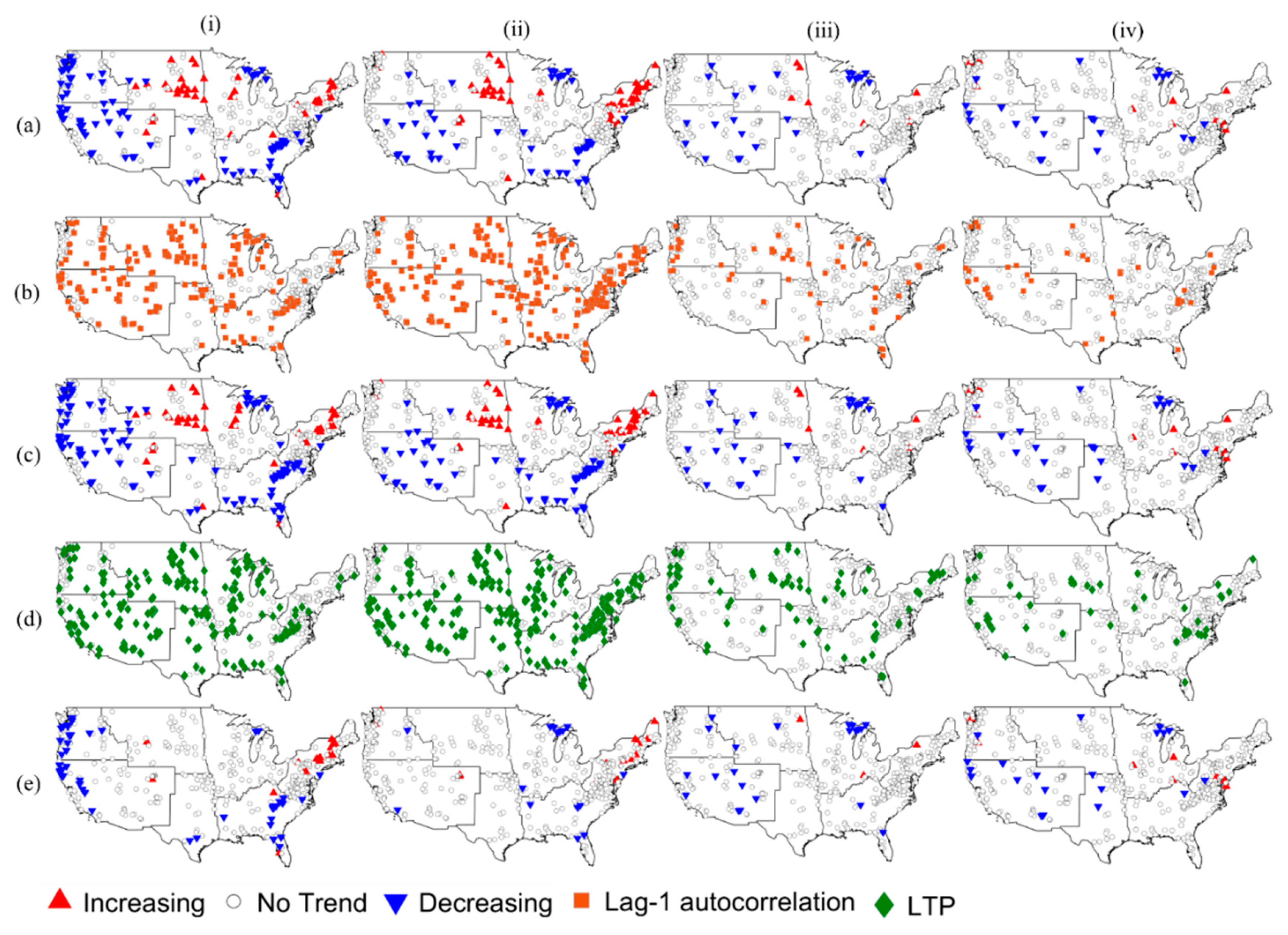
3.1.2. Trend in Percentile Streamflow

The results for MK1, MK2, and MK3 tend along with the serial correlation in (i) Q05, (ii) Q50, (iii) Q95, and (iv) Q100 for all climate regions within the contiguous US are presented in Figure 4. Row (a), (c), and (e) of Figure 4 shows the stations showing significant trend based on MK1, MK2, and MK3 tend, respectively. The upward/downward triangles represent the stations showing positive/negative trends. The number of stations within each climate region showing significant MK1, MK2, and MK3 trend for each percentile streamflow is summarized in Table 3. Table 3 also shows the regions which are field significant at p ≤ 0.1 with bold entries corresponding to the trend in percentile streamflow.
It was observed that a greater number of stations showed a trend in Q05 and Q50 flow while a very low number of stations showed a trend in Q95 and Q100 flow (Figure 4). Furthermore, few stations of NW, MW, and NE showed an increasing trend in high flows and the rest of the stations showed a decreasing trend in high flows. It was also observed that the MK1 and MK2 trends for Q05 and Q50 flows were field significant for all regions while the corresponding MK3 trend was not field significant. Furthermore, very few trend results for high flows were field significant. Although the spatial variation of stations showing a trend in high flows (Q95 and Q100) were like the spatial distribution of seasonal trends, very few stations showed a trend in high flows. The evaluated trend in the high flows is not consistent with the documented trend in precipitation [56] within the contiguous US, although precipitation is the key factor that governs streamflow. A significant flood has been observed in recent years, but the current study does not show a significant increasing trend in the high flows. This indicates that other factors like the soil moisture, changes in infiltration and time of concentration within a watershed may be governing parameters for determining the change in flood hydrology. Although not undergoing explicit analysis, Lins and Slack [15] have also indicated that the trend in 24-h precipitation with 100 mm or larger depth may have caused an increase in flooding. Unlike high flows, a greater number of stations showed a trend in low flow (Q05) and median streamflow (Q50). The decreasing trend in the Q05 and Q50 in the NW and SW indicates drier conditions causing hydrologic drought in the western US. Like the increasing trend in the seasonal streamflow of NE, the increasing trend in Q05 and Q50 can be attributed to the precipitation patterns and higher index of the North Atlantic Oscillation [57,58]. Again, the decreasing trend in the low flows in NW and SW signify the drier conditions in the western US caused by the reduction in snow cover and changes in snowmelt patterns of the region. In Figure 4b orange square markers represent the stations showing lag-1 autocorrelation. Similarly, green diamond markers in Figure 4d show the spatial location of stations showing LTP for respective percentile streamflow. Both lag-1 autocorrelation and LTP were detected in all climate regions. A higher number of stations showed lag-1 autocorrelation and LTP for Q05 and Q50 flows as compared to high flows. The spatial distribution of stations with lag-1 autocorrelation and LTP is shown in Figure 4b and Figure 4d, respectively.
Like the seasonal streamflow, the trend magnitude in percentile streamflow is also summarized in Figure 3 as the (%) percent change in the average metric. The changes were calculated based on the Thiel Sen slope like the calculations of seasonal streamflow corresponding to the stations showing the MK1 trend.

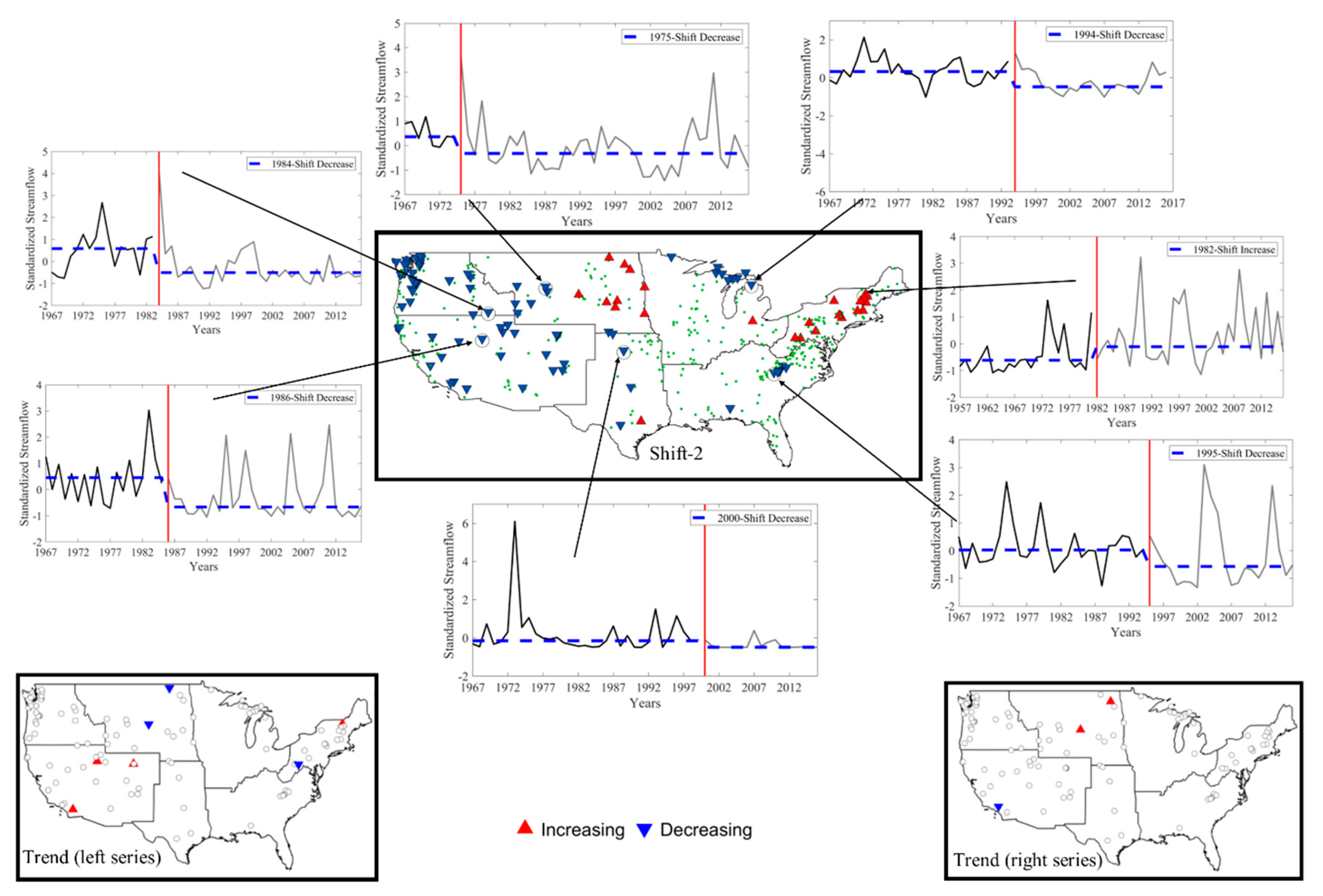
3.2. Shift and Trend-Shift Results

In this section, first, the results corresponding to seasonal and percentile streamflow are presented which include the evaluation of change point and the direction of shift followed by the trend evaluation before and after the occurrence of shift.
Figure 5 summarizes the change point (the year when the significant shift was detected) for seasonal and percentile streamflow. First, the change points corresponding to Shift-1 were computed followed by the change points corresponding to Shift-2 for both seasonal and percentile streamflow. All the circles in Figure 5 representing the change points are color-coded into six groups also representing the stations showing shift at the statistical significance of p ≤ 0.05. Each climate region showed uniformity in change points for seasonal streamflow after accounting for lag-1 autocorrelation (Shift-2) as compared to the change points before accounting for lag-1 autocorrelation (Shift-1). For example, three stations in NGP for (i) winter season represented by black circles showed shifts in the decade 2006–2016 before accounting for lag-1 (Shift-1), unlike Shift-2. Similarly, the colors of change point in SE are more uniform after accounting for lag-1 (Shift-2) as compared to the one before accounting for lag-1 autocorrelation (Shift-1). Similarly, stations of NW and SW showed more uniformity in change points for Q05 and Q50 flows after accounting for lag-1 autocorrelation (Figure 5). Similarly, for NGP and MW stations showed late shift (2006–2016) represented by black circles before accounting for lag-1 autocorrelation for Q05 and Q50 (Figure 5). After accounting for lag-1 autocorrelation (Shift-2), uniform change points were detected in NGP and MW for Q05 and Q50 flows as compared to the ones before accounting for lag-1 autocorrelation (Shift-1). This indicates that, similar to the seasonal streamflow volume, shift detection in percentile flows was also affected by the lag-1 autocorrelation and that trend free pre-whitening improves the shift result based on the uniformity in change point within each region.
The approach of trend free whitening to evaluate the shift was validated within the climate regions of the contiguous US. Such regional analysis showed some important results. It was observed that considering the lag-1 autocorrelation showed the coherence in the change points within each climate region and fewer stations showed shift after considering the lag-1 autocorrelation minimizing the shift overestimation. A smaller number of stations showed a significant shift after considering Lag-1 autocorrelation avoiding the overestimation of shift. The spatial distributions of the station showing both Shift-1 (before considering lag-1 autocorrelation) and Shift-2 (after considering lag-1 autocorrelation) were similar. Most of the shift have occurred during the decades 1976–1985 and 1986–1995. The shifts during 1976–1985 coincide with the regime shift during the period 1976–1977, when the climate of the Northern Pacific suddenly changed [20,21] and changes were observed in sardine population of the region [22,59]. The regime shift was caused by the coupled influence of solar forcing and planetary wave amplitude response [22] which impact different geophysical records. In the current study, such regime shifts were mostly observed in both seasonal and percentile streamflow within NW, SW, NGP, SGP, and MW during the period 1976–1985. Unlike these climate regions, stations of NE showed early shifts during the period 1966-1975.
MK1 trend was evaluated again before and after Shift-2 for the stations showing significant Shift-2. The streamflow data before the change point corresponding to Shift-2 is referred to hereafter as left series and the data after the change point is referred as the right series. The results for trend after accounting for Shift-2 for summer streamflow volume is summarized in Figure 6 and similar results were also obtained for other streamflow metrices. The central panel in Figure 6 shows the spatial distributions of streamflow stations showing significant Shift-2 in summer streamflow volume. The results of Shift-2 were similar to the trend results, the stations of the western US (NW and SW) showed decreasing shift during spring and summer while a greater number of stations showed decreasing shift in summer. Stations of NE showed an increasing shift during winter, summer, and autumn. Few stations of NGP and MW showed an increasing shift in all seasons.
Groisman et al. [52] documented the strong association between increased heavy precipitation and higher streamflow in the eastern United States. This explains the increasing shift within NE and NGP evaluated in the current study. The streamflow changes in the western US has been mostly documented as the changes in the streamflow peak timing caused by changes in snow cover and snowmelt patterns [49,60] possibly fading the higher streamflow caused by more frequent precipitation in the region [8]. This supports the decreasing shift and trend in both NW and SW evaluated in the current study during summer. Stations of NGP also showed an increasing trend, suggesting a higher correlation of the streamflow with the increased frequency of intense precipitation. It was observed that very few stations showed MK1 trend after accounting the shift for all streamflow metrices. It was also observed that a higher number of stations showed both Shift-1 and Shift-2 for Q05 and Q50 as compared to the high flows (Q95 and Q100). Previously, McCabe and Wolock [61] have documented significant changes in minimum and median daily streamflow as compared to maximum daily streamflow. As shown in Figure 6 for summer streamflow volume, very few stations showed trend in left series (bottom left panel) and right series (bottom right panel). This was true for all stations showing significant Shift-2 for all streamflow metrices. The seven time series plots represent the sample stations for each climate region; the vertical red lines represent the change point for each sample station. The black and grey time series plots in Figure 6 represent left series and right series, respectively, for the sample stations of each climate region. Spatial plots in the bottom left/right panel of Figure 6 represent the trend significance in the left series/right series, respectively. It can be seen that most of the stations did not show significant trend before and after the Shift year (change point). The dashed blue line in time series plots of Figure 6 represents the streamflow median in left and right series. A clear step in the streamflow median during the change point as shown in Figure 6 represents the shift in the streamflow for the sample stations of each region. Thus, it is important to clearly distinguish between trend and shift while evaluating the historic variability in streamflow which is also established by [23,61,62,63]. McCabe and Wolock [61] have also evaluated shifts in the streamflow of conterminous United States mostly occurring around 1970. The evaluated trend signifies that the changes will continue in future while, shift depicts that the historic changes are caused by regime shift in the climate system [61]. The novelty of the current research is that it also accounts for lag-1 autocorrelation and also evaluates the trend significance after considering Shift-2.
Furthermore, if the historic change in streamflow is completely caused by the long-term trend, it should also be present in both the original and split time series (left and right series). In the current study, for both the left series and right series, a smaller number of stations showed a significant trend as compared to the entire length of the data. This indicates the dominance of regime shift in the streamflow within the contiguous US as compared to the gradual trend in past records. Similar studies have also documented the regime shift in streamflow records [23,61]. Villarini et al. [23] indicated that shift should be evaluated before analyzing the trend. There should be a clear distinction among trend and shift to attribute whether the variability is caused by long term variability and/or the variability is caused by abrupt shift Villarini et al. [23]. Similarly, Pathak et al. [63] has documented more shifts as compared to trends in the hydrological variability of the Midwestern United States. The current study was performed over the entire contiguous United States. Additionally, the evaluation of significant shift and change points in the current study was improved by considering the lag-1 autocorrelation as mention earlier. The current study also evaluated the trend after splitting the streamflow records before and after the change point to verify whether the variability is associated to regime shift or long-term trend. Based on the current results, regime shift is more likely to reoccur in streamflow as compared to gradual changes if the hydrologic variability remains consistent in the future.

4. Conclusions

The regional analysis of streamflow was performed by grouping 419 unimpaired stations into 7 climate regions based on NCA recommendation. The Walker test was performed to assess the global field significance corresponding to each climate region to understand whether the evaluated regional trend and shift are by change or are globally significant. The study was performed on 50 years of seasonal streamflow volume and percentile streamflow records for all regions except for NE with 60 years of records. At first, some stations of NGP and MW showed an increasing trend and shift in spring–summer streamflow while some remaining stations showed a decreasing trend and shift. Later, a comprehensive study of streamflow variability was performed for four seasonal streamflow volumes (winter, spring, summer, and autumn) and four yearly streamflow percentiles (Q05, Q50, Q95, and Q100). The observations made by the current study are enlisted below:
  • The trend in streamflow varied spatially with the climate regions and the number of stations showing trend also differed with seasons. A greater number of stations showed a trend during summer as compared to other seasons. Stations of NE showed an increasing trend in streamflow while stations of NW and SW showed a decreasing streamflow trend during summer.
  • A greater number of stations showed a trend in Q05 and Q50 as compared to Q95 and Q100. Stations of NGP and NE showed an increasing trend while stations of NW and SW showed a decreasing trend in Q05 and Q50. Very few stations with a decreasing trend in Q100 were scattered over all climate regions except for a few stations of NE and MW showing an increasing trend.
  • Both LTP and lag-1 autocorrelation were observed in seasonal streamflow volume and percentile streamflow. LTP influenced the trend significance of streamflow more than lag-1 autocorrelation as a smaller number of stations showed the MK3 trend as compared to the MK1 and MK2 trends. The maximum number of stations of NW and SW showed decreasing MK1, MK2, and MK3 summer streamflow trend; this suggests the changes in streamflow within the region are not caused by long term variability rather may be attributed to the recent changes caused by changing climate.
  • A smaller number of stations showed a shift in both seasonal streamflow volume and percentile streamflow after accounting for lag-1 autocorrelation. Accounting for lag-1 autocorrelation improved the results of change point; stations within each climate regions showed more uniformity in change points after accounting for lag-1 autocorrelation.
  • A smaller number of stations showed a trend in both seasonal and percentile streamflow records after accounting for the shift. This shows the changes in streamflow are the result of regime shift as compared to the long-term trends.
The current study provides detailed insights of historic streamflow variability within the climate regions of the contiguous United States and can be helpful for the water managers to make useful decisions. The current study can be extended to explain the cause of the observed trend and shift by identifying the physical drivers.

Author Contributions

Conceptualization, A.K.; investigation, B.T.; software, B.T, and R.J.; formal analysis, B.T., and N.J.; supervision, A.K.; writing—original draft preparation, B.T., N.J., R.T., and A.K.; writing—review and editing, B.T., N.J., R.J., R.T., and A.K. All authors have given approval to the final version of the manuscript.

Funding

This research received no external funding.

Acknowledgments

The authors would like to thank the editor and three anonymous reviewers for constructive feedback. The authors would like to acknowledge HCDN and NCA for public data access. The authors would like to acknowledge the Doctoral Fellowship Award provided by the graduate school at Southern Illinois University, Carbondale.

Conflicts of Interest

The authors declare no conflict of interest.

References

  1. Nazemi, A.; Wheater, H.S. Assessing the Vulnerability of Water Supply to Changing Streamflow Conditions. Eos Trans. Am. Geophys. Union 2014, 95, 288. [Google Scholar] [CrossRef]
  2. Bridgewater, P.; Guarino, E.; Thompson, R. Hydrology in the Anthropocene. Encycl. Anthr. 2018, 87–92. [Google Scholar] [CrossRef]
  3. Joshi, N.; Kalra, A.; Lamb, K.W. Land–Ocean–Atmosphere Influences on Groundwater Variability in the South Atlantic–Gulf Region. Hydrology 2020, 7, 71. [Google Scholar] [CrossRef]
  4. Deb, P.; Kiem, A.S.; Willgoose, G. A linked surface water-groundwater modelling approach to more realistically simulate rainfall-runoff non-stationarity in semi-arid regions. J. Hydrol. 2019, 575, 273–291. [Google Scholar] [CrossRef]
  5. IPCC. Summary for Policymakers. In Global Warming of 1.5 °C. An IPCC Special Report on the Impacts of Global Warming of 1.5 °C above Pre-Industrial Levels and Related Global Greenhouse Gas Emission Pathways, in the Context of Strengthening the Global Response to the Threat of Climate Change, Sustainable Development, and Efforts to Eradicate Poverty; Masson-Delmotte, V.P., Zhai, H.-O., Pörtner, D., Roberts, J., Skea, P.R., Shukla, A., Pirani, W., Moufouma-Okia, C., Péan, R., Pidcock, S., et al., Eds.; World Meteorological Organization: Geneva, Switzerland, 2018; p. 32. [Google Scholar]
  6. Durdu, Ö.F. Effects of climate change on water resources of the Büyük Menderes River basin, western Turkey. Turk. J. Agric. Forest. 2010, 34, 319–332. [Google Scholar]
  7. Milly, P.C.D.; Betancourt, J.; Falkenmark, M.; Hirsch, R.M.; Kundzewicz, Z.W.; Lettenmaier, D.P.; Stouffer, R.J. Stationarity is Dead: Whither Water Management? Science 2008, 319, 573–574. [Google Scholar] [CrossRef]
  8. Solander, K.C.; Reager, J.T.; Wada, Y.; Famiglietti, J.S.; Middleton, R.S. GRACE satellite observations reveal the severity of recent water over-consumption in the United States. Sci. Rep. 2017, 7, 1–8. [Google Scholar] [CrossRef] [Green Version]
  9. NCEI. NOAA National Centers for Environmental Information. U.S. Billion-Dollar Weather and Climate Disasters. Available online: http://www.ncdc.noaa.gov/billions/summary-stats (accessed on 5 May 2020). [CrossRef]
  10. Mallakpour, I.; Villarini, G. Investigating the relationship between the frequency of flooding over the central United States and large-scale climate. Adv. Water Resour. 2016, 92, 159–171. [Google Scholar] [CrossRef] [Green Version]
  11. Mallakpour, I.; Villarini, G. The changing nature of flooding across the central United States. Nat. Clim. Chang. 2015, 5, 250–254. [Google Scholar] [CrossRef]
  12. Shukla, S.; Safeeq, M.; AghaKouchak, A.; Guan, K.; Funk, C. Temperature impacts on the water year 2014 drought in California. Geophys. Res. Lett. 2015, 42, 4384–4393. [Google Scholar] [CrossRef] [Green Version]
  13. AghaKouchak, A.; Cheng, L.; Mazdiyasni, O.; Farahmand, A. Global warming and changes in risk of concurrent climate extremes: Insights from the 2014 California drought. Geophys. Res. Lett. 2014, 41, 8847–8852. [Google Scholar] [CrossRef] [Green Version]
  14. Shrestha, A.; Rahaman, M.; Kalra, A.; Thakur, B.; Lamb, K.W.; Maheshwari, P. Regional Climatological Drought: An Assessment Using High-Resolution Data. Hydrology 2020, 7, 33. [Google Scholar] [CrossRef]
  15. Lins, H.F.; Slack, J.R. Streamflow trends in the United States. Geophys. Res. Lett. 1999, 26, 227–230. [Google Scholar] [CrossRef] [Green Version]
  16. Sagarika, S.; Kalra, A.; Ahmad, S. Evaluating the effect of persistence on long-term trends and analyzing step changes in streamflows of the continental United States. J. Hydrol. 2014, 517, 36–53. [Google Scholar] [CrossRef]
  17. Hamlet, A.F.; Lettenmaier, D.P. Effects of Climate Change on Hydrology and Water Resources in the Columbia River Basin. JAWRA J. Am. Water Resour. Assoc. 1999, 35, 1597–1623. [Google Scholar] [CrossRef]
  18. Thakur, B.; Kalra, A.; Ahmad, S.; Lamb, K.W.; Lakshmi, V. Bringing statistical learning machines together for hydro-climatological predictions—Case study for Sacramento San joaquin River Basin, California. J. Hydrol. Reg. Stud. 2020, 27, 100651. [Google Scholar] [CrossRef]
  19. Serinaldi, F.; Kilsby, C.G. The importance of prewhitening in change point analysis under persistence. Stoch. Environ. Res. Risk Assess. 2015, 30, 763–777. [Google Scholar] [CrossRef] [Green Version]
  20. Kerr, R.A. Unmasking a Shifty Climate System. Science 1992, 255, 1508–1510. [Google Scholar] [CrossRef] [Green Version]
  21. Gedalof, Z.; Mantua, N.J.; Peterson, D.L. A multi-century perspective of variability in the Pacific Decadal Oscillation: New insights from tree rings and coral. Geophys. Res. Lett. 2002, 29, 57-1. [Google Scholar] [CrossRef] [Green Version]
  22. Powell, A.M., Jr.; Xu, J. The 1977 Global Regime Shift: A Discussion of Its Dynamics and Impacts in the Eastern Pacific Ecosystem. Atmos. Ocean 2012, 50, 421–436. [Google Scholar] [CrossRef]
  23. Villarini, G.; Serinaldi, F.; Smith, J.A.; Krajewski, W.F. On the stationarity of annual flood peaks in the continental United States during the 20th century. Water Resour. Res. 2009, 45, 45. [Google Scholar] [CrossRef]
  24. Bunting, A.H.; Dennett, M.D.; Elston, J.; Milford, J.R. Rainfall trends in the West African Sahel. Q. J. R. Meteorol. Soc. 1976, 102, 59–64. [Google Scholar] [CrossRef]
  25. Thakur, B.; Kalra, A.; Lakshmi, V.; Lamb, K.W.; Miller, W.P.; Tootle, G. Linkage between ENSO phases and western US snow water equivalent. Atmos. Res. 2020, 236, 104827. [Google Scholar] [CrossRef]
  26. Hamed, K.H. Trend detection in hydrologic data: The Mann–Kendall trend test under the scaling hypothesis. J. Hydrol. 2008, 349, 350–363. [Google Scholar] [CrossRef]
  27. Regonda, S.K.; Rajagopalan, B.; Clark, M.; Pitlick, J. Seasonal Cycle Shifts in Hydroclimatology over the Western United States. J. Clim. 2005, 18, 372–384. [Google Scholar] [CrossRef]
  28. Helsel, D.R.; Hirsch, R.M. Statistical Methods in Water Resources; Elsevier: Amsterdam, The Netherlands, 1992; p. 49. [Google Scholar]
  29. Kendall, M. Multivariate Analysis; Charles Griffin: London, UK, 1975; p. 210. [Google Scholar]
  30. Mann, H.B. Nonparametric Tests against Trend. Econometrica 1945, 13, 245. [Google Scholar] [CrossRef]
  31. Yue, S.; Pilon, P.; Phinney, B.; Cavadias, G. The influence of autocorrelation on the ability to detect trend in hydrological series. Hydrol. Process. 2002, 16, 1807–1829. [Google Scholar] [CrossRef]
  32. Von Neumann, J. Distribution of the Ratio of the Mean Square Successive Difference to the Variance. Ann. Math. Stat. 1941, 12, 367–395. [Google Scholar] [CrossRef]
  33. Alexandersson, H. A homogeneity test applied to precipitation data. J. Clim. 1986, 6, 661–675. [Google Scholar] [CrossRef]
  34. Pettitt, A.N. A Non-Parametric Approach to the Change-Point Problem. J. R. Stat. Soc. Ser. C Appl. Stat. 1979, 28, 126. [Google Scholar] [CrossRef]
  35. Wijngaard, J.B.; Tank, A.M.G.K.; Können, G.P. Homogeneity of 20th century European daily temperature and precipitation series. Int. J. Clim. 2003, 23, 679–692. [Google Scholar] [CrossRef]
  36. Hurst, H.E. Long-term storage capacity of reservoirs. Trans. Am. Soc. Civil Eng. 1951, 116, 770–808. [Google Scholar]
  37. Koutsoyiannis, D.; Montanari, A. Statistical analysis of hydroclimatic time series: Uncertainty and insights. Water Resour. Res. 2007, 43. [Google Scholar] [CrossRef]
  38. Yue, S.; Pilon, P. A comparison of the power of the ttest, Mann-Kendall and bootstrap tests for trend detection/Une comparaison de la puissance des teststde Student, de Mann-Kendall et du bootstrap pour la détection de tendance. Hydrol. Sci. J. 2004, 49, 21–37. [Google Scholar] [CrossRef]
  39. Melillo, J.M.; Richmond, T.C.; Yohe, G. Climate Change Impacts in the United States: The Third National Climate Assessment; U.S. Global Change Research Program: Washington, DC, USA, 2014; p. 841.
  40. Bosilovich, M.G. Regional Climate and Variability of NASA MERRA and Recent Reanalyses: U.S. Summertime Precipitation and Temperature. J. Appl. Meteorol. Clim. 2013, 52, 1939–1951. [Google Scholar] [CrossRef]
  41. Schoof, J.T.; Ford, T.W.; Pryor, S.C. Recent Changes in U.S. Regional Heat Wave Characteristics in Observations and Reanalyses. J. Appl. Meteorol. Clim. 2017, 56, 2621–2636. [Google Scholar] [CrossRef]
  42. Lins, H.F. USGS Hydro-Climatic Data Network 2009 (HCDN-2009). In Fact Sheet; U.S. Geological Survey: Washington, DC, USA, 2012; p. 4. [Google Scholar]
  43. Theil, H. A Rank-Invariant Method of Linear and Polynomial Regression Analysis. Adv. Stud. Theor. Appl. Econom. 1992, II, 345–381. [Google Scholar] [CrossRef]
  44. Sen, P.K. Estimates of the regression coefficient based on Kendall’s tau. J. Am. Stat. Assoc. 1968, 63, 1379–1389. [Google Scholar] [CrossRef]
  45. Wilks, D.S. On “Field Significance” and the False Discovery Rate. J. Appl. Meteorol. Clim. 2006, 45, 1181–1189. [Google Scholar] [CrossRef]
  46. Redmond, K.T.; Koch, R.W. Surface Climate and Streamflow Variability in the Western United States and Their Relationship to Large-Scale Circulation Indices. Water Resour. Res. 1991, 27, 2381–2399. [Google Scholar] [CrossRef]
  47. Zhang, Y.; Schilling, K. Increasing streamflow and baseflow in Mississippi River since the 1940s: Effect of land use change. J. Hydrol. 2006, 324, 412–422. [Google Scholar] [CrossRef]
  48. Miles, E.L.; Snover, A.K.; Hamlet, A.F.; Callahan, B.; Fluharty, D. Pacific Northwest Regional Assessment: The Impacts of Climate Variability and Climate Change on the Water Resources of the Columbia River Basin1. JAWRA J. Am. Water Resour. Assoc. 2000, 36, 399–420. [Google Scholar] [CrossRef] [Green Version]
  49. Kunkel, K.E.; Palecki, M.A.; Ensor, L.; Easterling, D.; Hubbard, K.G.; Robinson, D.; Redmond, K. Trends in Twentieth-Century U.S. Extreme Snowfall Seasons. J. Clim. 2009, 22, 6204–6216. [Google Scholar] [CrossRef]
  50. Pathak, P.; Kalra, A.; Ahmad, S. Temperature and precipitation changes in the Midwestern United States: Implications for water management. Int. J. Water Resour. Dev. 2016, 33, 1003–1019. [Google Scholar] [CrossRef]
  51. De Martino, G.; Fontana, N.; Marini, G.; Singh, V.P. Variability and Trend in Seasonal Precipitation in the Continental United States. J. Hydrol. Eng. 2013, 18, 630–640. [Google Scholar] [CrossRef]
  52. Groisman, P.Y.; Knight, R.W.; Karl, T.R. Heavy Precipitation and High Streamflow in the Contiguous United States: Trends in the Twentieth Century. Bull. Am. Meteorol. Soc. 2001, 82, 219–246. [Google Scholar] [CrossRef] [Green Version]
  53. Arheimer, B.; Donnelly, C.; Lindström, G. Regulation of snow-fed rivers affects flow regimes more than climate change. Nat. Commun. 2017, 8, 1–9. [Google Scholar] [CrossRef] [Green Version]
  54. Hamed, K.H.; Rao, A.R. A modified Mann-Kendall trend test for autocorrelated data. J. Hydrol. 1998, 204, 182–196. [Google Scholar] [CrossRef]
  55. Khaliq, M.N.; Ouarda, T.B.M.J.; Gachon, P.; Sushama, L. Temporal evolution of low-flow regimes in Canadian rivers. Water Resour. Res. 2008, 44, 44. [Google Scholar] [CrossRef] [Green Version]
  56. Karl, T.R.; Knight, R.W.; Plummer, N. Trends in high-frequency climate variability in the twentieth century. Nat. Cell Biol. 1995, 377, 217–220. [Google Scholar] [CrossRef]
  57. Hurrell, J.W.; Van Loon, H. Decadal variations in climate associated with the North Atlantic Oscillation. Clim. Chang. 1995, 31, 301–326. [Google Scholar]
  58. Hurrell, J.W. Decadal Trends in the North Atlantic Oscillation: Regional Temperatures and Precipitation. Science 1995, 269, 676–679. [Google Scholar] [CrossRef] [PubMed] [Green Version]
  59. Kawasaki, T. Why do some pelagic fishes have wide fluctuations in their numbers? Biological basis of fluctuation from the viewpoint of evolutionary ecology. FAO Fish 1983, 291, 1065–1080. [Google Scholar]
  60. Prein, A.F.; Rasmussen, R.M.; Ikeda, K.; Liu, C.; Clark, M.P.; Holland, G.J. The future intensification of hourly precipitation extremes. Nat. Clim. Chang. 2017, 7, 48–52. [Google Scholar] [CrossRef]
  61. McCabe, G.J.; Wolock, D.M. A step increase in streamflow in the conterminous United States. Geophys. Res. Lett. 2002, 29, 38-1. [Google Scholar] [CrossRef]
  62. Solander, K.C.; Bennett, K.E.; Middleton, R.S. Shifts in historical streamflow extremes in the Colorado River Basin. J. Hydrol. Reg. Stud. 2017, 12, 363–377. [Google Scholar] [CrossRef]
  63. Pathak, P.; Kalra, A.; Ahmad, S.; Bernardez, M. Wavelet-Aided Analysis to Estimate Seasonal Variability and Dominant Periodicities in Temperature, Precipitation, and Streamflow in the Midwestern United States. Water Resour. Manag. 2016, 30, 4649–4665. [Google Scholar] [CrossRef]
Figure 1. Map showing the locations of 419 unimpaired streamflow within National Climate Assessment regions (1—Northwest, 2—Southwest, 3—Northern Great Plains, 4—Southern Great Plains, 5—Midwest, 6—Northeast, and 7—Southeast). The map also shows 18 United States Geological Survey Hydrologic Unit catchments along with major rivers.
Hydrology 07 00091 g001
Figure 2. Maps showing results for trend, lag-1 autocorrelation, and long-term persistence (LTP) for (i) winter, (ii) spring, (iii) summer, and (iv) autumn streamflow volume. Row (ae) summarizes MK1, Lag-1, MK2, LTP and MK3 results, respectively. All the stations showing (increasing/decreasing) the trend at the statistical significance of p ≤ 0.05 are represented by the (upward/downward) triangles. Squares and diamonds represent the station showing lag-1 autocorrelation and LTP. Circles represent the absence of a trend, lag-1 autocorrelation and LTP.
Hydrology 07 00091 g002
Figure 3. Box plots for the percent change in streamflow based on the Thiel–Sen slope. The percent change is calculated based on the average value of the streamflow metric during the study period. The boxes represent the distribution of the trend between 25th and 75th percentiles and the medians are represented by horizontal red lines. The outliers at 5th and 95th percentiles are shown as the whiskers.
Hydrology 07 00091 g003
Figure 4. Maps showing results for trend, lag-1 autocorrelation, and long-term persistence (LTP) for (i) 5th percentile, (ii) 50th percentile, (iii) 95th percentile, and (iv) 100th percentile streamflow. Row (ae) summarizes MK1, Lag-1, MK2, LTP and MK3 results, respectively. All the stations showing a (positive/negative) trend at the statistical significance of p ≤ 0.05 are represented by the (upward/downward) triangles. Square and diamond markers represent the stations showing lag-1 autocorrelation and LTP, respectively. Circles represent the absence of a trend, lag-1 autocorrelation and LTP.
Hydrology 07 00091 g004
Figure 5. Maps showing change points for seasonal and percentile streamflow corresponding to both Shift-1 and Shift-2.
Hydrology 07 00091 g005
Figure 6. A spatial plot of stations showing significant Shift-2 is shown in the central panel. The spatial plots in the bottom left/right panel represent the trend significance in the left series/right series, respectively. The seven time series plots represent the sample stations of each climate region; the vertical red line represents the change point for each sample station. The dark and grey lines in the time series plots represent the left series and right series, respectively. The dashed blue lines represent the change in median streamflow in the left and right series. All the plots represent summer streamflow volume. The upward/downward triangles represent increasing/decreasing trend and Shift-2 at the statistical significance of p ≤ 0.05.
Hydrology 07 00091 g006
Table 1. National Climate Assessment (NCA) regions of the Contiguous US and their constituent states along with the selected number of streamflow stations within each NCA region.
S.N.NCA RegionsNo. of StationsConstituent States
1Northwest (NW)56Idaho, Oregon, Washington
2Southwest (SW)76California, Nevada, Utah, Arizona, New Mexico, Colorado
3Northern Great Plains (NGP)41Kansas, Nebraska, South Dakota, North Dakota, Wyoming, Montana
4Southern Great Plains (SGP)29Texas, Oklahoma
5Midwest (MW)58Ohio, Indiana, Michigan, Illinois, Wisconsin, Missouri, Iowa, Minnesota
6Northeast (NE)65Maine, Vermont, New Hampshire, Massachusetts, New York, Rhode Island, Connecticut, New Jersey, Pennsylvania, Maryland, Delaware, Washington DC, West Virginia
7Southeast (SE)94Virginia, Kentucky, Tennessee, Arkansas, Mississippi, Alabama, Louisiana, Georgia, Florida, South Carolina, North Carolina
Table 2. Results for the Mann–Kendall (MK) test along with Pettitt Shift before/after accounting lag-1 autocorrelation (Shift-1 /Shift-2) for seasonal streamflow. The entries in bold identify the region was field significant at p ≤ 0.1.
Winter Spring Summer Autumn
Trend (+/−)Shift (+/−)Trend (+/−)Shift (+/−)Trend (+/−)Shift (+/−)Trend (+/−)Shift (+/−)
MK1MK2MK3Shift-1 Shift-2MK1MK2MK3Shift-1Shift-2MK1MK2MK3Shift-1Shift-2MK1MK2MK3Shift-1Shift-2
Midwest1/11/10/03/12/16/85/86/74/84/82/72/72/61/101/95/35/34/14/114/11
Northeast11/011/09/018/117/11/61/61/61/30/322/120/120/117/015/020/019/014/022/015/0
Northern Great Plains8/18/21/013/18/14/15/10/17/36/310/49/42/312/79/715/114/15/018/414/2
Northwest0/10/10/00/10/10/20/20/10/20/20/260/270/250/290/263/23/23/11/21/2
Southeast0/50/70/50/360/360/110/120/100/130/150/60/70/60/70/70/30/30/30/30/3
Southern Great Plains0/20/10/02/21/10/30/30/10/20/21/31/30/21/51/50/20/20/12/22/2
Southwest11/49/66/113/310/50/130/120/110/140/130/260/250/220/240/243/123/142/34/182/14
Table 3. Results for the Mann–Kendall (MK) test along with Pettitt Shift before/after accounting lag-1 autocorrelation (Shift-1 /Shift-2) for streamflow percentiles. The entries in bold identify that the region was field significant at p ≤ 0.1.
Q05Q50Q95Q100
Trend (+/−)Shift(+/−)Trend (+/−)Shift(+/−)Trend (+/−)Shift(+/−)Trend (+/−)Shift(+/−)
MK1MK2MK3Shift-1Shift-2MK1MK2MK3Shift-1Shift-2MK1MK2MK3Shift-1Shift-2MK1MK2MK3Shift-1Shift-2
Midwest5/75/100/23/121/102/92/90/72/91/91/81/81/72/92/93/43/43/43/23/2
Northeast17/117/117/120/120/132/127/111/145/132/12/02/01/02/02/04/14/13/14/14/1
Northern Great Plains18/216/41/020/315/416/116/10/022/313/34/43/31/37/84/70/10/10/12/22/2
Northwest6/210/210/161/250/252/22/22/11/50/50/10/20/11/20/23/13/22/16/26/2
Southeast2/302/352/152/312/300/210/320/50/250/300/20/20/20/40/40/20/20/10/60/5
Southern Great Plains1/31/30/25/43/41/11/10/03/32/20/20/20/00/30/30/40/40/30/50/5
Southwest4/275/271/126/284/265/163/172/14/202/160/90/90/80/70/70/90/90/90/70/5
Publisher’s Note: MDPI stays neutral with regard to jurisdictional claims in published maps and institutional affiliations.

