A New Automatic Monitoring Network of Surface Waters in Greece: Preliminary Data Quality Checks and Visualization

Abstract

The monitoring of surface waters is of fundamental importance for their preservation under good quantitative and qualitative conditions, as it can facilitate the understanding of the actual status of water and indicate suitable management actions. Taking advantage of the experience gained from the coordination of the national water monitoring program in Greece and the available funding from two ongoing infrastructure projects, the Institute of Inland Waters of the Hellenic Centre for Marine Research has developed the first homogeneous real-time network of automatic water monitoring across many Greek rivers. In this paper, its installation and maintenance procedures are presented with emphasis on the data quality checks, based on values range and variability tests, before their online publication and dissemination to end-users. Preliminary analyses revealed that the water pH and dissolved oxygen (DO) sensors and produced data need increased maintenance and quality checks respectively, compared to the more reliably recorded water stage, temperature (T) and electrical conductivity (EC). Moreover, the data dissemination platform and selected data visualization options are demonstrated and the need for both this platform and the monitoring network to be maintained and potentially expanded after the termination of the funding projects is highlighted.

1. Introduction

Automatic telemetric monitoring stations in surface water bodies can provide nowcasting and early warning services, essential for pollution mitigation and preparation against extreme events [1,2,3,4,5]. Automatic monitoring provides very large volumes of data in high temporal and spatial resolution, allowing the detection of both short-term events and long-term changes, thus contributing significantly to environmental research [6,7,8]. Wireless technologies make it possible to connect to remote areas, enabling very fast data transmission from local metering stations to data processing centers. Moreover, the latest technological developments of in situ sensors and telecommunication protocols provide continuous data flows at low operational and maintenance costs, increasing the feasibility of establishing permanent, large-scale monitoring networks [9,10,11].

Despite the global development of water monitoring programs based on seasonal sampling, real-time water quality monitoring networks at a relatively large scale (regional and national) are not widespread. Many automatic networks are small and are deployed at the local level, usually in basin areas with high management needs. The largest example of continuous monitoring is the national US network, which is comprised of >2000 stations that provide real-time measurements of the common water parameters of pH, temperature (T), electrical conductivity (EC) and dissolved oxygen (DO) [12]. As far as the European Union (EU) monitoring program is concerned, the EU Water Framework Directive (WFD) requires that all member countries monitor their water bodies on a seasonal basis towards the achievement of “good status” [13], with water information from the pan-European network of “sampling-sites” being stored in databases [14]. Continuous monitoring of water that allows for immediate water-quality information available in real-time is not part of the EU legislation and any efforts to install and operate automatic stations or networks of stations arise from individual interest in each country.

The Institute of Marine Biological Resources and Inland Waters (IMBRIW) of the Hellenic Centre for Marine Research (HCMR) is in charge of coordinating the national surface water monitoring program in Greece, under the supervision of the General Secretariat of Water of the Ministry of Environment, Energy and Climate Change [15]. Systematic water sampling is carried out on a seasonal basis from hundreds of river sites across the country to evaluate their water status with respect to physicochemical and biological conditions [15]. However, seasonal monitoring cannot guarantee the early identification of sudden water deterioration in rivers that can disturb the aquatic life and degrade the quality of the water distributed to users from downstream nodes. This service can only be provided with automatic monitoring instruments measuring water parameters in real time. A network of stations with automatic instruments is still missing from the Greek territory, as its development has not been centrally coordinated so far. Only few sparse efforts have been carried out by educational and research institutes or local water management authorities, with limited geographical and temporal application. Thus, many existing automatic monitoring stations with valuable data have been abandoned, others do not operate appropriately due to inadequate maintenance or the use of outdated measuring technologies, while in most of them data are fragmented and remain undisclosed [16].

Automatic monitoring networks offer important services but are also vulnerable to malfunctions, mostly due to inevitable damage of sensors, which can cause data loss or degradation. Nevertheless, measures can be taken to ensure the appropriate operation of the instruments, and improve the quality of data provided to end users through data checks and evaluations. Quality assurance and quality control (QA/QC) is in practice a set of automated methods for the identification and correction of problematic measurements, including graphs and statistics useful for evaluation [17]. More precisely, a QA is defined as a set of procedures that minimize inaccuracies in the data generated due to factors like natural phenomena or malicious human activity, such as theft or vandalism, data corruption during transmission, etc. [18], while QC refers to the actual procedures that are implemented as part of the QA plan after data collection, where the incorrect data are identified, labeled and potentially excluded or corrected before their public availability [19,20]. In fact, the need for automated and standardized approaches to QA/QC has increased since the monitoring systems have now entered the era of “big data” [21,22,23,24].

The appropriate design and operation of an automatic monitoring network relies on a number of factors including, among others, the environmental and research objectives and the development and dissemination of relevant products, the representativeness of the monitoring locations and water variables, and the effectiveness and efficiency of QA/QC procedures [25,26]. The network should also be planned within the current institutional setting and budgetary and logistical constraints. Within this context, in the design of a monitoring network in Greece one has to consider the need to comply with the environmental legislation in Europe in a cost-effective manner, covering first the geographical areas of high and medium priority. Such areas can be defined as the landscapes where river water bodies do not yet meet the “good status” required by the WFD [13] or the ones of particular environmental and socioeconomic importance, which could benefit more from an intense monitoring.

Recently, the HCMR has surveyed the existing network of automatic water quality stations in Greek rivers and, by applying a GIS-based multicriteria decision analysis approach, it has identified the existing monitoring needs along with the priority areas for the installation and operation of automatic, telemetric stations [16]. Taking advantage of the financial support under two relevant research projects, HIMIOFoTS [27] and OpenELIoT [28], 15 stations have been established across Greece in 2019 and 2020. These stations were added to the three sparsely established stations from 2014 to 2016, funded from previous projects, raising the total number of HCMR stations, up to now, to 18, located in 11 rivers. The HIMIOFoTs project aims to create an integrated infrastructure for the management of the Greek national water resources, which is expected to provide important services both to the scientific community and to the society by providing open access to data from marine and inland waters monitoring networks, and to related forecasting products that may lead to the development of added value products and services [27]. The OpenELIoT project aims to implement an integrated and economically viable Internet of Things solution for monitoring and analyzing surface water parameters, in an economically efficient way [28]. In both projects, data quality checks and visualization are integrated in online platforms, being freely available to end users and the public.

Both projects that support the development of the automatic monitoring network are still ongoing, with a few more stations being planned to be installed in the coming years. Ideally, a few more years of operation would be needed for an integrated assessment of the network, including optimized procedures of data quality control and publication/visualization. However, the current progress allows a preliminary evaluation, which can offer the opportunity to receive constructive feedback. Hence, this article presents the development of the first centrally coordinated effort to establish a national network for real-time monitoring of surface water bodies in Greece, along with the necessary maintenance procedures and the quality checks on data before their transfer to the publication platforms.

2. Methodology

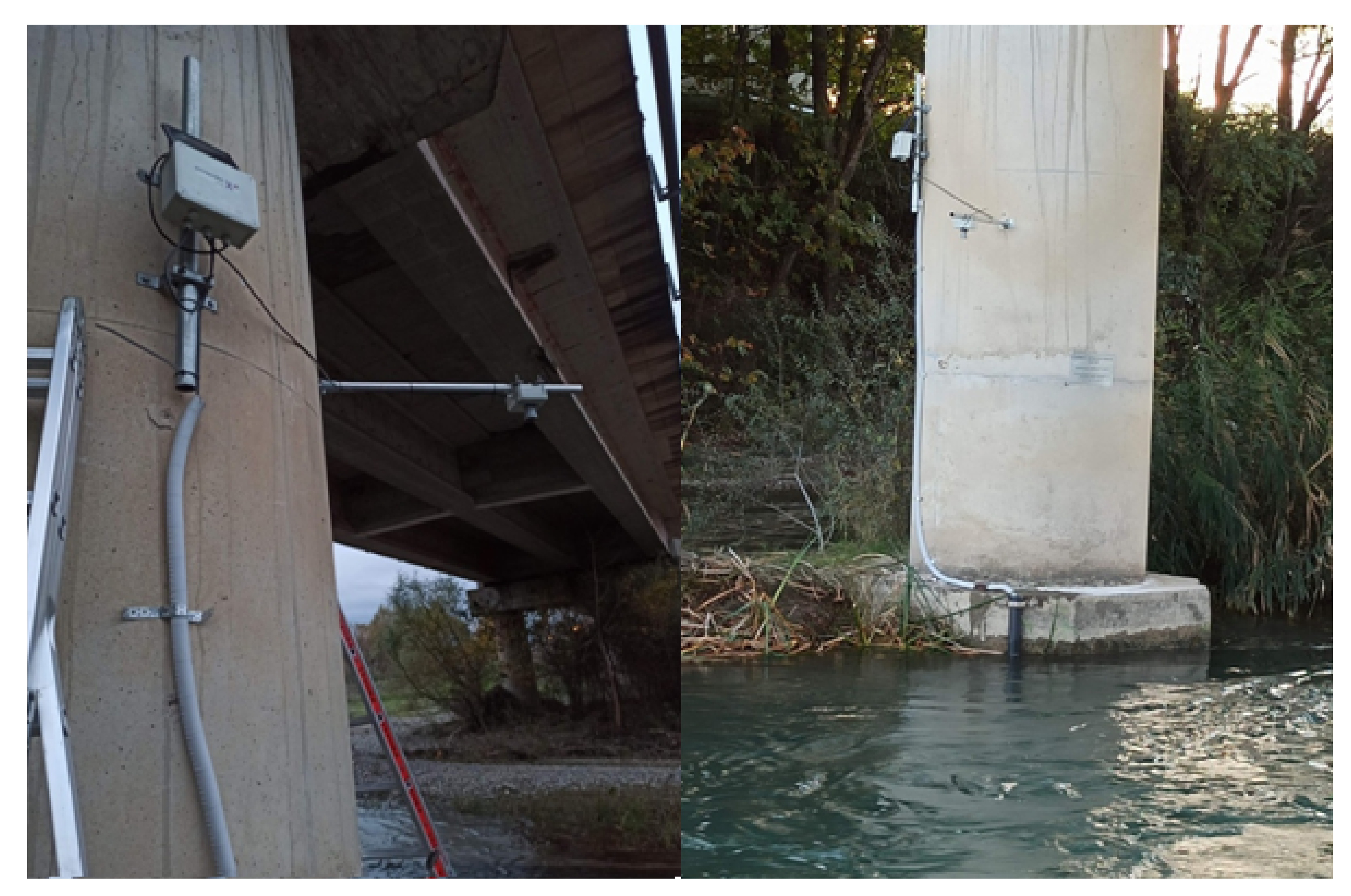
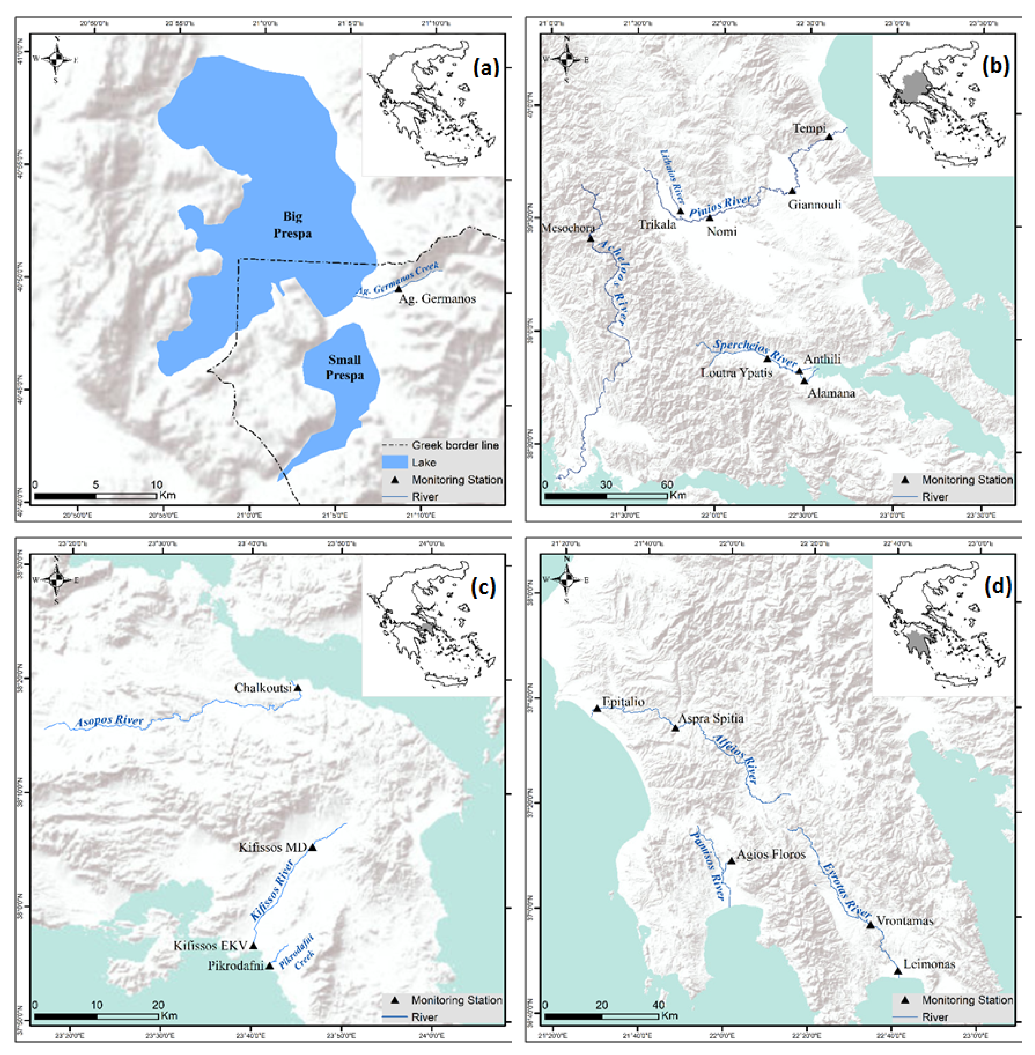
2.1. The HCMR Network: Stations Selection, Locations and Technical Specifications

The 18 established automatic monitoring stations in rivers of Greece measure water stage and four physicochemical parameters of water: pH, T, EC and DO. Stage is practically the basis for determining river discharge and thus is important for evaluating the water quantity conditions in the river, especially with a focus on low flow (drought) and high flow (flood) conditions. The other four physicochemical parameters give a general but instructive overview of the river’s water quality and are all important for assessing and understanding the biogeochemical processes of surface water ecosystems [29]. All these parameters are directly measurable through a single instrument with all the respective sensors adapted on it. In particular, the main component of the HCMR stations is the sonde In-Situ Aqua TROLL 400 (AT400), which is described in terms of the manufacturer’s specifications in

Table 1. In-Situ AT400 manufacturer specifications [30].

Parameter	Accuraccy	Range	Resolution
Water level	Typical ± 0.1% FS @ 15 °C; ±0.3% FS max. from 0 to 50 °C	76 m	±0.01% FS or better
Electrical Conductivity (EC)	Typical ± 0.5% + 1 μS/cm; ±1% max.	5 to 100,000 μS/cm	0.1 μS/cm
Dissolved Oxygen (DO)	±0.1 mg/L from 0 to 20 mg/L; ±2% of reading from 20–60 mg/L	0–60 mg/L	0.01 mg/L
pH	±0.1 pH unit from 0 to 12 pH units	0 to 14 pH units	0.01 pH unit
Temperature (T)	±0.1 °C	−5 to 50 °C (23 to 122 °F)’	0.01 °C or better

.

The HCMR stations are installed under bridges as shown in Figure 1. The solar panel used for the power supply of the water station was placed at a high point with abundant sunlight on the vertical abutment (pier column), while the instrument with the sensors was placed in the water in a safe position near the pier’s bottom.

If economically and technically feasible, it is preferred to deploy at least two stations per river catchment, one in its upper part, even close to its headwaters, and the second downstream close to the mouth. In this way, having as a reference the expected good water quality conditions at the upper part, a comparison of water quality parameters for the same time period between the two stations will allow the identification of pollution sources in the intermediate catchment. Another important benefit is the opportunity to assess the time needed for severe hydrometeorological events, which are usually more intense in the upstream (and mountainous) part of a catchment, to affect the downstream lowland catchment where economic activities are mostly developed. Figure 2 depicts the 18 sites and the 11 smaller or larger rivers where HCMR stations have already been deployed, while

Table 2. The HCMR automatic water quality monitoring stations up to December 2020.

Water District	River	Site Name	Coordinates (φ, λ)	Started from	Research Project
Eastern Central Greece	Spercheios	Alamana	38.81250, 22.49520	3/7/2014	HIMIOFoTS
Eastern Central Greece	Spercheios	Anthili	38.85611, 22.46685	4/7/2014	HIMIOFoTS
Eastern Central Greece	Spercheios	Loutra Ypatis	38.907822, 22.283958	27/11/2019	OpenELIoT
Western Central Greece	Acheloos	Mesochora	39.42010, 21.26261	29/7/2016	HIMIOFoTS
Thessaly	Pinios	Giannouli	39.65246, 22.40780	25/8/2019	HIMIOFoTS
Thessaly	Pinios	Nomi	39.52657, 21.93833	26/8/2019	HIMIOFoTS
Thessaly	Pinios	Tempi	39.89675, 22.61520	25/8/2019	HIMIOFoTS
Western Peloponnese	Alfeios	Aspra Spitia	37.58641, 21.79087	1/8/2019	HIMIOFoTS
Western Peloponnese	Alfeios	Epitalio	37.64256, 21.47648	1/8/2019	HIMIOFoTS
Western Peloponnese	Pamisos	Agios Floros	37.168887, 22.024621	25/9/2020	OpenELIoT
Eastern Peloponnese	Evrotas	Vrontamas	36.973848, 22.580371	21/7/2020	OpenELIoT
Eastern Peloponnese	Evrotas	Leimonas	36.828865, 22.691026	21/7/2020	OpenELIoT
Attica	Kifissos	Kifissos MD	38.091799, 23.781160	8/7/2020	OpenELIoT
Attica	Kifissos	Kifissos EKV	37.947538, 23.672446	15/7/2020	OpenELIoT
Attica	Pikrodafni	Pikrodafni	37.922411, 23.700816	1/10/2019	OpenELIoT
Eastern Central Greece	Asopos	Chalkoutsi	38.324726, 23.753182	3/7/2020	OpenELIoT
Thessaly	Lithaios	Trikala	39.552411, 21.770816	21/11/2019	OpenELIoT
Western Macedonia	Ag. Germanos (Prespa Lake)	Ag. Germanos	40.836957, 21.140266	13/7/2020	OpenELIoT

Note: Water Districts are large River Basin Areas including several smaller watersheds. Greece is divided into 14 Water Districts. The “Alamana”, “Anthili” and “Mesochora” stations were installed a few years before 2019 within the framework of previous funding projects but they are assigned to the “HIMIOFoTS” project on the table due to their recent upgrade with economic sources from this project.

summarizes useful information related to their location and operation.

2.2. Stations Maintenance and Data Checks

So far, there is no universal QA/QC procedure for examining data validity and optimizing data quality, but only common automatic practices, especially for data errors detection. The development of the HCMR network of automatic stations follows common data quality checks that have been proposed in the literature [17,31,32], after extensive testing.

The main sources of errors in the water physicochemical data are the deposition of biological or other material on the sensors (sensors biofouling/fouling) and the deviation of the sensors (sensors drift). Drift is the natural tendency of a sensor to change its characteristics over time, due to aging of materials and/or due to environmental changes (in temperature and humidity), resulting in changes of the output signal, while the measured physical quantity remains stable. Other sources of error are damage to sensors, recorders and/or data transmission systems, and unpredictable environmental conditions that can affect the operation of measuring instruments [19,29].

As a result, a station can provide erroneous data such as: (a) measurements out of the permissible range of values for the recording parameter, (b) persisting values of a measured parameter, usually because of a damage causing the datalogger to record continuously the last measurement, and (c) no measurements or measurements equal to zero due to a failure of the sensor or datalogger or due to a power outage or battery damage resulting in abnormal data recording. It should be also noted that incorrect measurements at a constant value could also be attributed to an erroneous calibration [19].

Regular inspection and maintenance of the monitoring stations is taking place by experienced HCMR personnel in frequencies that fluctuate from monthly to quarterly. All sondes are subject to routine cleaning, so that their sensors will not become coated with biofilm, sediment and other debris, and calibration process against standards. Quality checks are performed during each site visit through comparison readings with a HANNA 98194 field reference sonde, temporarily deployed to determine sensors’ drift. The field reference sonde is carefully maintained and checked before use against laboratory standards and calibrated as needed. The deviations of the stations recordings from the respective in situ measurements are calculated and statistically elaborated. Box-plots and frequency histograms are used to present the level of deviation occurring per water quality parameter and season, and to investigate if any relation exists between the magnitude of deviation and the calibration frequency of the sensors.

Every site station incorporates sensors and recording systems for the measurement of the parameters at regular intervals, ensuring almost continuous recording of the state of the water, which can be processed and published directly on the internet. The data from the sensors are transferred telemetrically (via GPRS) to a server at time intervals ranging from 10 min to 1 h (usually 30 min and 1 h are preferred), they are stored in databases and are published both as raw and quality checked data on the HIMIOFoTS [27] and OpenELIoT [28] projects platforms and on an HCMR central visualization platform [33], which combines all stations from both projects. It is worth mentioning that data logger’s clock is set to standard time (UTC) to avoid confusion during the transition to or from daylight saving time.

For the needs of the data quality checks of the HCMR network a two-stage procedure is followed. As a first step, algorithms apply plausibility tests to observations with a pass/fail criterion based on predetermined allowable data ranges and variability to detect possibly erroneous values [17,32]. In a second stage suspicious values are labeled using specific flags and examined through graphs by qualified scientists, who judge whether these measurements represent extreme natural phenomena and should be integrated in the entire data series without labeling or whether they are of poor quality and have to remain flagged.

Prior to all data checks, a date/time test is performed to ensure that the data correspond to successive recorded values based on the selected time step (e.g., hourly). This is immediately followed by a check of zero measurements and/or empty values, which leave all these records empty before the next tests are applied. Incorrect records in the raw data transmitted from a network station usually have the word “null” or a high negative value (e.g., −9999) or even a zero, when it cannot be referred to a real measurement. In the present network, for whatever reason and for any duration an instrument does not record the variable, the respective raw data are left blank, but even sporadic normal values within an extended empty period are not excluded and pass a further quality check.

Then, for the remaining values, a range test is first performed in order to identify values outside the expected natural limits of each variable, considering the instruments limits and the physical ranges of the corresponding variable. A test of extreme values (extreme value test) follows by simply marking the greatest and smallest values within the entire data set, and a test of extreme differences of successive values within the data set (extreme difference test), which indicates for further observation the largest and smallest absolute changes of consecutive observations. Finally, the data quality check includes a persistence test, which examines whether or not a variable has stopped varying with time, indicating a non-response of the sensor to changes in the values of the variable (stuck value test). The tests implemented in the water quality data recorded by the automatic stations of HCMR were further analyzed.

The range test ensures that the measurements are within allowable limits.

Table 3. Physiochemical parameters recorded in Greek rivers and their permissible limits.

Water Parameter	Unit	Min	Max
Temperature (T)	(°C)	0	30
Electrical Conductivity (EC)	(μS/cm)	30	5000
pH	(-)	5	10
Dissolved Oxygen (DO)	(mg/L)	4	11

gives the upper and lower bound of each parameter used in our range quality check, which did not coincide to the absolute natural variability but represent smaller, expected ranges that are practically not exceeded in the aquatic environment of Greek rivers.

The priority here is that labeling correct data due to the strictest limits and confirm them as acceptable in the second stage (graph observation) is preferable than not labeling poor quality data due to wider allowable ranges and passing them through the first stage tests, unflagged.

Checking for possible erroneous extreme values that do not necessarily lie outside the above limits is further done by marking the 2.5% highest and the 2.5% lowest recorded values of the data set, excluding those values that have already been marked according to the “out-of-range” criterion. This further draws our attention to the 5% of the remaining values for inspection and in combination with the already “out-of-range” labeled values is expected to represent the vast majority of possible errors. Therefore, the criterion of labeling a fixed percentage of 5% of the “within-the-permissible-range” recorded values helps in the cases that even the acceptable limits of Table 3 represent rather wide ranges that can allow the non-flagging of extreme values or outliers that should be flagged. Therefore, this extreme value check flags a standard 5% of the values of the data set (with out-of-range values excluded), comprised of its 2.5% lower values and 2.5% higher values. For example, in a data set with 100,000 hourly or subhourly values after the range test, the 5000 most extreme values (5%) will be highlighted.

With a similar approach, the variability of the data was examined. We calculated the absolute differences of the consecutive recorded values (after excluding the out-of-range ones) and indicated the 2.5% lowest values and the 2.5% highest values. The flagged 5% of absolute differences allows one to graphically examine if the highest and lowest consecutive (1 h or 30 min) changes correspond to abnormal patterns of unnatural fluctuations. In both the above tests, the number of flagged values that represent the 5% subset of the “within-the permissible-range” data, increases as the database is populated with new measurements and the corresponding limits change dynamically by recalculating the corresponding percentiles every time new data gets into the database.

The last check of the data is done to see if there is a so-called “freeze” in the measurement data or otherwise if a value is stuck and does not change for many consecutive recordings. As far as the water quality parameters: pH and DO are concerned, the fluctuations in each time step can be almost zero for quite a long time (hours) and, thus, such a criterion may lead to long flagging, without necessarily indicating problematic measurements. After experimentation, a complete absence of change (absolutely zero) for a two-days duration was selected for both pH and DO and was extended to the other two water quality parameters of T and EC. In practice, the sum of the absolute differences of the last two days (48 measurements for hourly values or 96 for half-hourly values) is checked against zero. This test is called a “stuck value test” or “persistent value test”.

Table 4. The quality tests applied in the data recorded by the automatic stations of HCMR.

Problem	Reliability Check	Type of Data	Definition
Empty record Multiple empty records	Null test Gap test	Missing data or long time period with missing data	Leave empty records
Implausible values	Range test	Extreme values	Min and Max limits of Table 3
Extreme values (within plausible range of observations)	Extreme value test	Extreme values	2.5% smallest and 2.5% largest observations
Extreme value differences (within plausible range of observations)	Extreme difference test	Differences (absolute) of consecutive pairs of values	2.5% smallest and 2.5% largest absolute consecutive differences of the observations
Persistent values (within plausible range of observations)	Stuck value test	Consecutive differences (absolute) of consecutive pairs of values	Zero change of the last 48 1 h or 96 half-hour recorded values

summarizes the quality control checks implemented for the monitoring network of HCMR.

It has to be noted that data can be flagged from more than one test. For example, a raw observation may be out of the 95% range of the observations, but its absolute difference from the previous observation may be out of the 95% difference range too. Actually, sometimes flagged values due to the stuck value test may have been flagged already from the previous test since the zero changed values also belong to the 2.5% least changed values (smallest differences). The stuck value test however has to predominate as the zero change implies a more serious malfunction (shown next).

Graphs are an important and easy tool for evaluating data. Values that are identified by the quality checks as suspicious should be marked on the graph (parameter vs. time) with a different color or symbol, while the blank entries will leave corresponding gaps in the graph. For flagged data in the graphs, it will be judged whether these measurements should be removed due to poor quality or if they are rather normal values and must be maintained.

3. Results

3.1. Application of Quality Checks on Real-Time Data and Flagging

The automatic station “Mesochora” (Acheloos River) (see Figure 2 and Table 2) was chosen for presenting representative graphs of the HCMR stations network and of the followed data quality check procedures. The station measures continuously the water parameters: stage, pH, T, EC and DO and transmits its instantaneous measurements to the data center every hour. For visualization purposes a shorter than the whole operation period is selected for display here, starting from 01/08/2018 and lasting 20 months. Actually, the Mesochora site is from the oldest HCMR monitoring sites (see Table 2), but the selected time-period covers a representative range of data recording malfunctions to present herein.

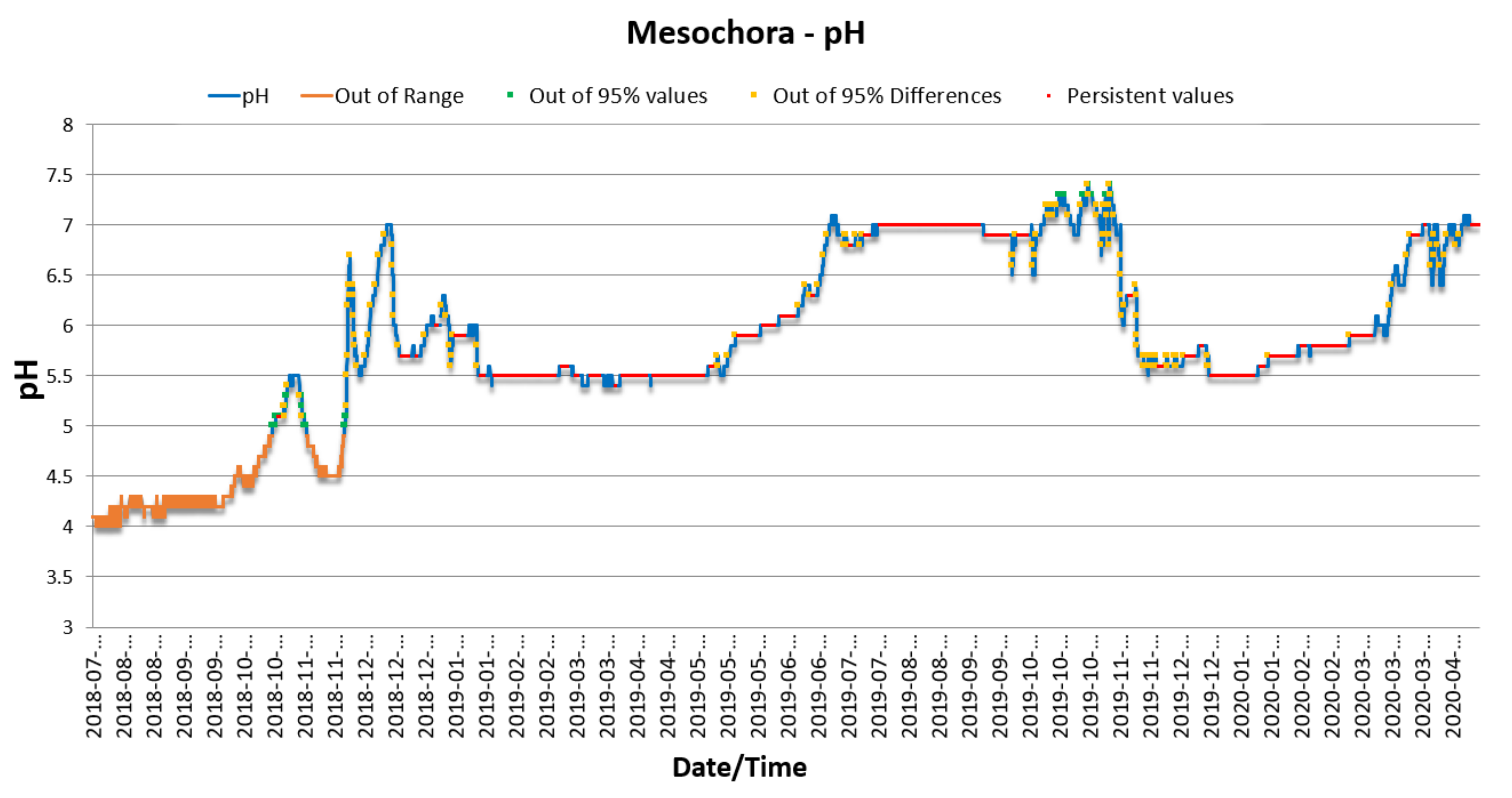
3.1.1. Evaluation Based on pH Data Quality Checks

Figure 3 depicts the pH graph at an hourly time step from August 2018 until April 2020 including flagged data as they were marked by the automatic checks applied. For the 20-month period selected, a 0.6% of the total expected 1 h observations of pH are empty records.

The measurements that passed the quality checks without being indicated with any possible error were 43.59%. Almost 84% of the recorded values were within the allowable limits of this parameter (5 < pH < 10, see Table 3), while when checking for possible persistent values for an extended period, possible errors were detected in about 37% of the measurements, which makes this type of error the most important and most common in the pH data set. At the left part of the graph the orange color results from the implementation of the range test. The test found that for a long period of more than two months all the recorded values were out of range, specifically pH was less than 5 (lower allowable bound), which did not allow further examination with one of the other tests. Then, a period with more acceptable values of pH began that lasted until early 2019. For the remaining “within-the-permissible-limits” raw data, the selected tests detected the 5% of the values, which lay below the 2.5% and above 97.5% percentiles (green), and outside the respective percentiles of the value differences (yellow). For the former and specifically for the above 97.5% values, which were found in late 2019 and were all close to pH = 7, there did not seem to be any suspicious recording. The 2.5% lowest pH values appeared at the end of 2018 and were slightly greater than five succeeding the period with out-of-range values. These “green” values are however suspicious and should not be uncolored. The yellow symbols are interchanged with normal blue values, indicating fluctuations for further observation. In fact, all yellow symbols in Figure 3 corresponded to the 2.5% larger sequential (1 h) differences and should be carefully observed for potential unexpected hourly pH increases/decreases. On the other hand, the rest of the 2.5% of “yellow” data, representing the minimum hourly changes, are “lost” under the persistent values that are marked with the stuck value test. Indeed, measurements that persist at specific values for a long time (red color) are observed in several parts of the graph indicating that the sensor was probably not working properly and was stuck many times within the 20-month period. Obviously, the 2.5% lowest changes were zero changes that coincided with persistent values checked with red. As shown in Figure 3, the zero changes in pH values for long periods were met more in 2019 but continued in 2020, sometimes for shorter periods and sometimes for longer ones. The sensor returned to normal function mostly after a calibration and/or a maintenance visit to the station. Overall, the pH graph of Figure 3 for the Mesochora station shows problematic behavior that needs to be further interpreted through station and sensor checks.

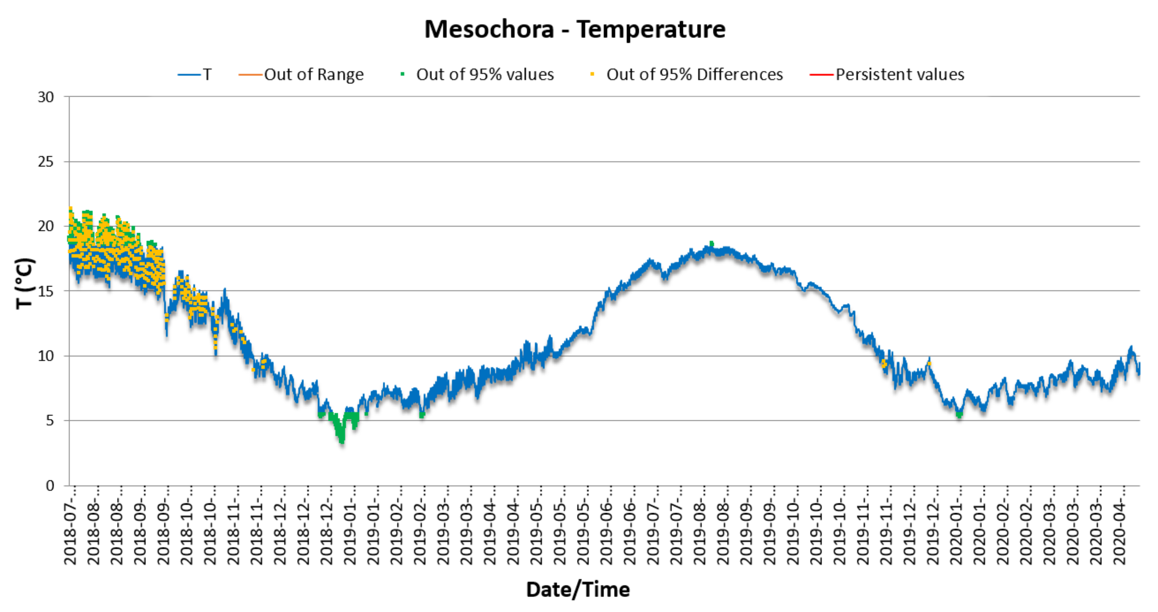
3.1.2. Evaluation Based on Temperature (T) Data Quality Checks

The vast majority of T measurements passed the quality checks without being indicated with any possible error. In fact, only the extreme value test and the extreme difference test marked values of this data set, as expected. Figure 4 illustrates the change in T on an hourly time step over the study period. The graph at first glance refers to normal T fluctuations, with values above 15 °C in the summer months that fell even below 5 °C in the winter months. The tests did not indicate any values outside the allowable range of Table 3 for T (0–30 °C) or “frozen” (persistent) values. So, only the small percentage of 5% of observations were highlighted representing the 2.5% higher and 2.5% lower observations and higher/lower absolute differences respectively. Attention in this graph is required more for the latter than for the former. Possible large hourly changes in summer 2018 have to be evaluated by experienced staff to determine if they are consistent with changes in ambient temperature. The highest temperatures over the 20-month period are indicated with green color on the same part of the graph being overlapped with the greatest fluctuations in consecutive differences. The highest actual temperatures did not however seem to be abnormal since they were slightly above 20 °C, a level that was normally reached during a hot summer in Mediterranean river systems. It is generally believed that water temperature is measured very reliably and it is rather rare to detect systematic or even sparse errors. It is also important to notice that no gaps were observed in the T diagram, a sign that the sensor could work without problems for long periods.

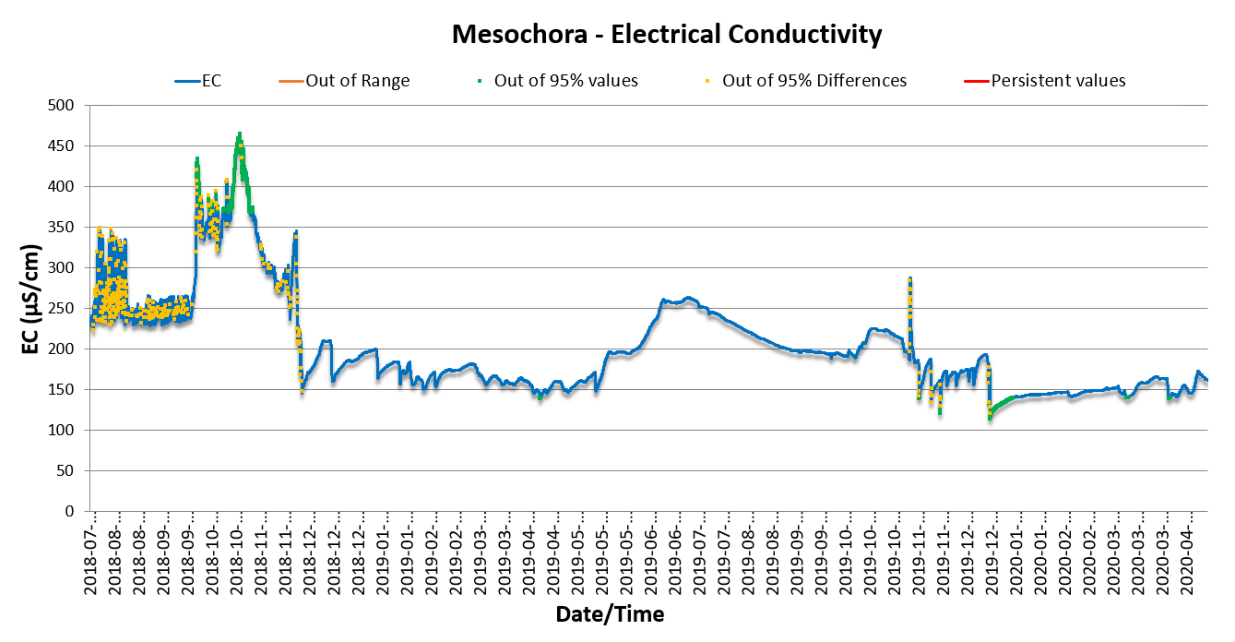
3.1.3. Evaluation Based on Electrical Conductivity (EC) Data Quality Check

Similarly with T, the vast majority of EC measurements passed the quality checks without being indicated with any possible error, with only the extreme value and extreme difference value tests, as normally expected, leading to marked values of this data set. Figure 5 illustrates the change in EC on an hourly time step over the study period. The values of the parameter and the differences of its successive values that are outside the 2.5–97.5% percentiles have been labeled. There are no out-of-range or persistent values as mentioned above. The most notable in the graph is the yellow area at the beginning where rather high hourly changes (increases/decreases) occur repeatedly and indicate either a sensor problem or a recurring episode of pollution. In general, the EC appears from the graph to be measured quite reliably for a long time.

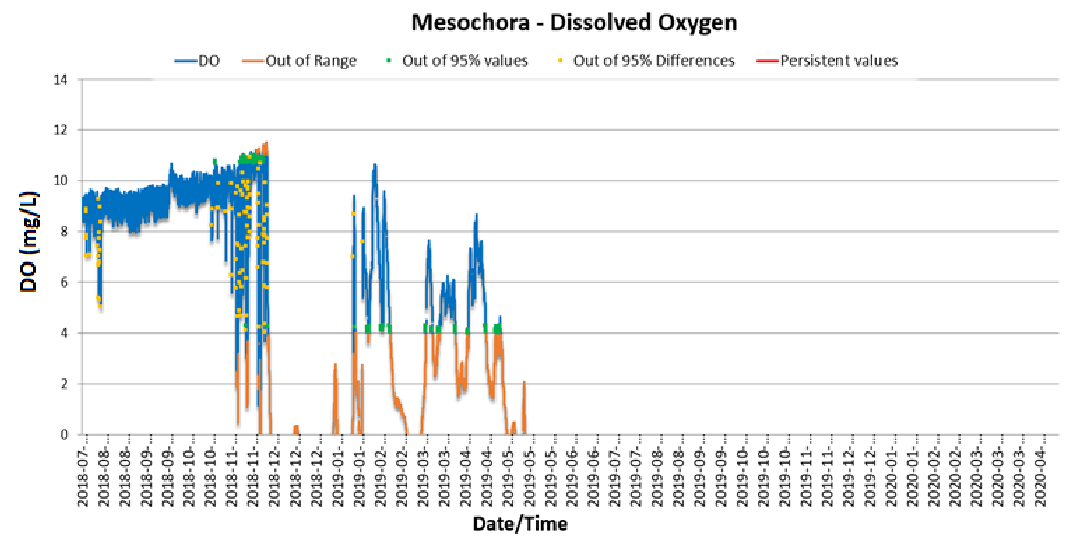
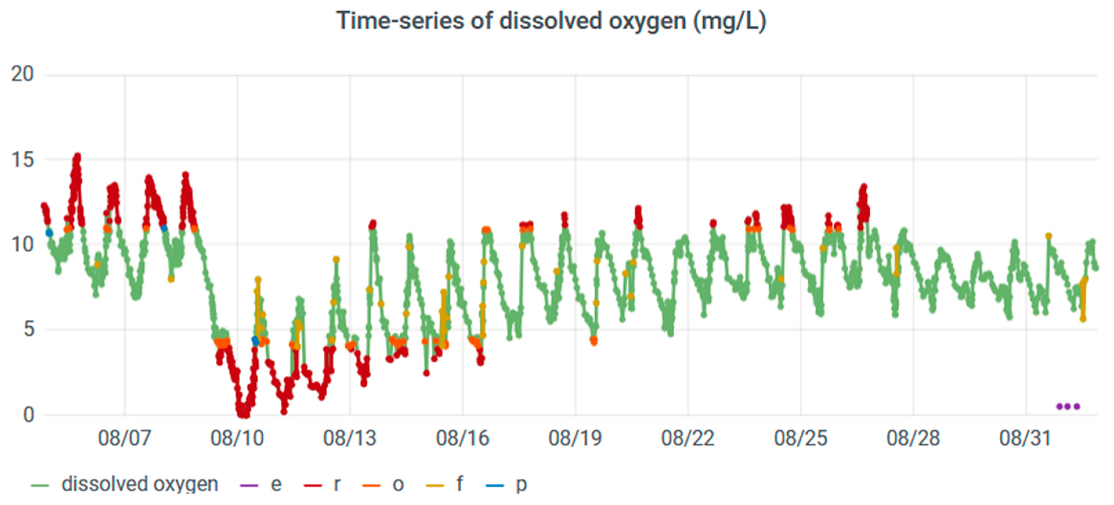
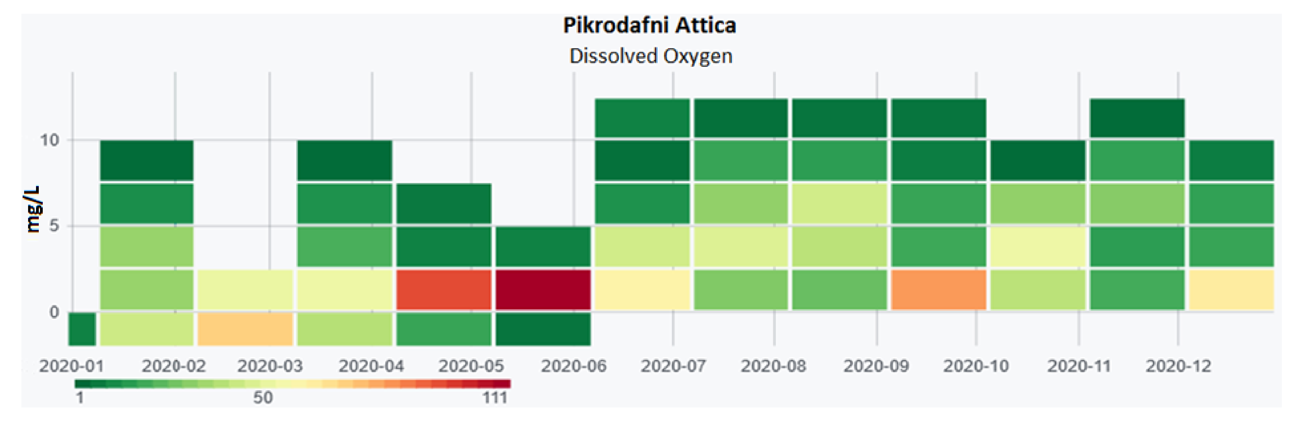
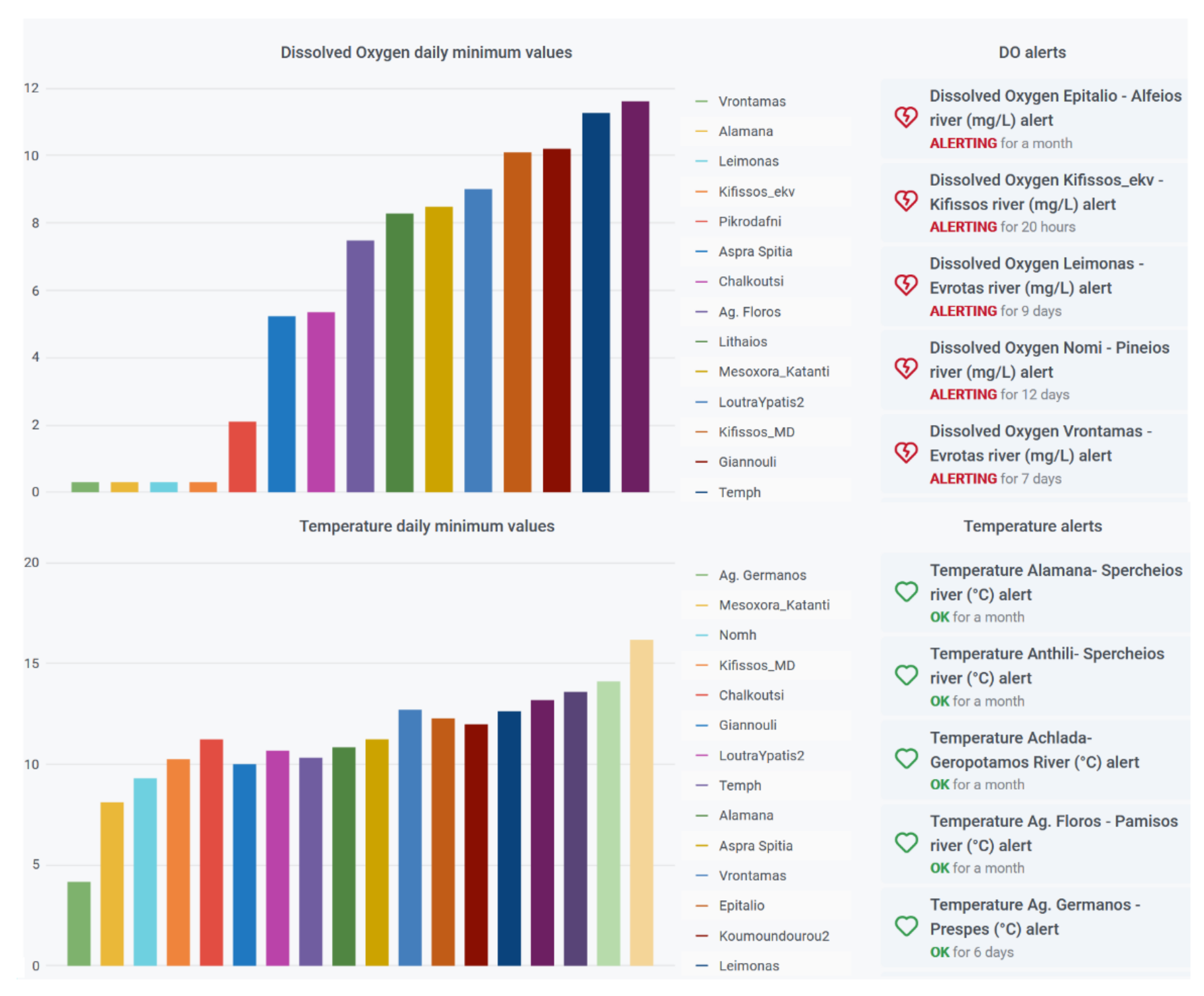
3.1.4. Evaluation Based on Dissolved Oxygen (DO) Quality Check

On the contrary, the majority of DO hourly records within the 20-month period of interest did not pass any quality check as records from May 2019 and onwards were empty. Moreover, a significant percentage of the recorded values before May 2019 are possibly in error. As shown in Figure 6, there are significant parts of the time series outside the allowable range (orange color). These erroneous data are systematically observed in the graph where many values lie below the lower limit, even reaching zero. However, the measurements return within the allowable limits, which means that the sensor works, implying that a phenomenon (probably pollution) causes the DO high fluctuations. There is a period at the end of 2018 characterized by the largest fluctuations in successive value differences (yellow color), which though, based on the general behavior of the parameter, may be reasonable. The biggest problem of the data set is the long period with empty values (non-recording), which essentially indicates the shutdown of the sensor. This happened as shown in the graph in May 2019 and can be attributed either to a problem with the sensor itself or with a station damage/removal. However, as other parameters have been recorded during the same period, it is obvious that the station suffers from a DO sensor failure that was not repaired until the end of the 20-month study period. Overall, the graph of Figure 6 for the Mesochora station reveals a rather suspicious operation of the DO sensor with no recording for almost a year and with high fluctuations lying out of allowable limits when recording. The DO sensor is characterized by low durability and needs more frequent maintenance/calibration or even replacement.

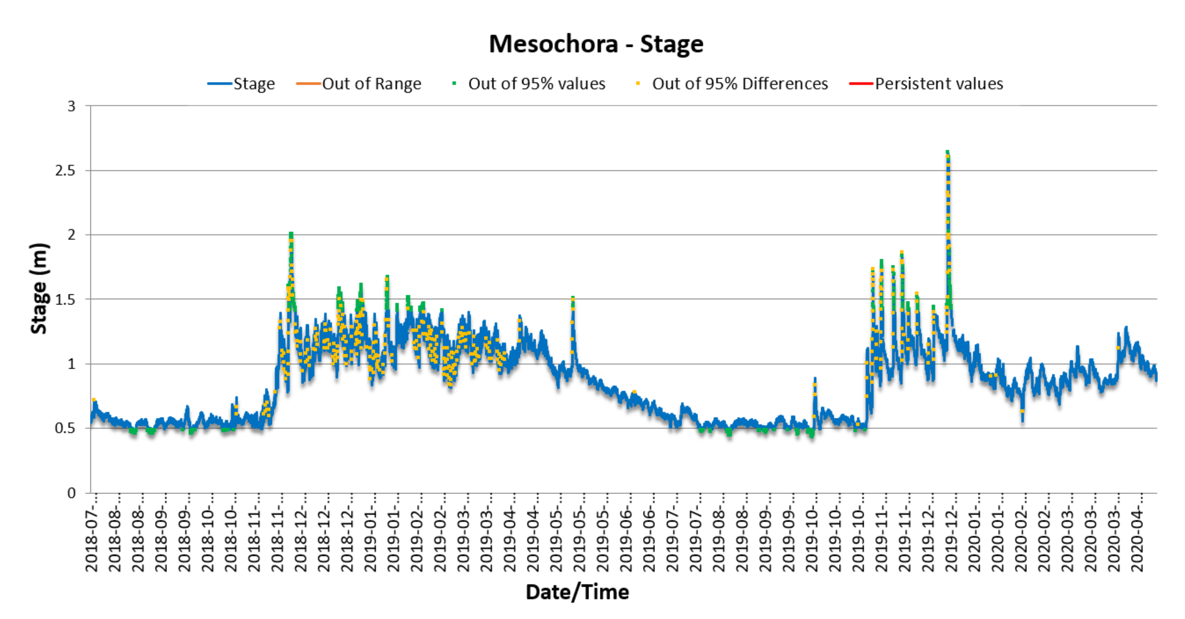
3.1.5. Evaluation of Water Level Measurements

To enhance the interpretation of the water quality graphs above, the stage of water in Mesochora station is presented in Figure 7, where the water level fluctuations are shown for the same 20-month period. The graph at Mesochora station was complete (no gaps) and represents a typical stage graph with high flow peaks (high water levels) alternating systematically with lower flows (low water levels). Only the 5% greatest/lowest values and 5% greatest/lowest differences were identified. An extra quality check that an expert could do with this graph is to inspect the occurrence of peaks by comparing them with local precipitation measurements to confirm their validity. Persistent values are absent as expected when the water level monitoring instrument works properly, while out-of-range values could only be detected at a higher level than 4–5 m, which however cannot be defined homogenously across the monitoring network as in the case of the water quality parameters. There is confidence that no errors are present at the water level graph.

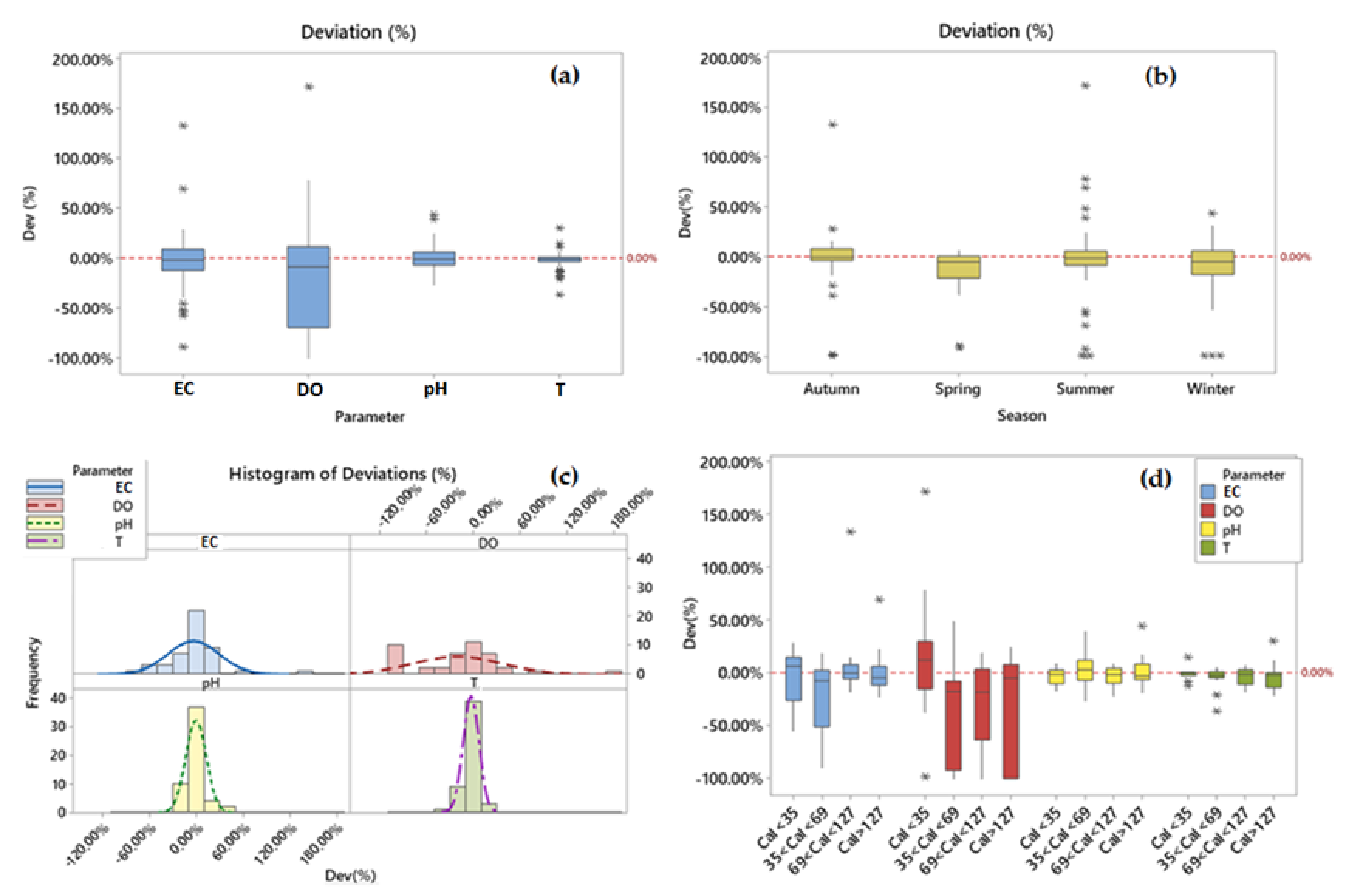
3.2. Statistical Analyses of the Deviations of Stations Recordings from in Situ Measurements

During each site visit, readings with a field reference sonde are compared with the respective records of the automatic station. The percentage deviations between in situ measurements and stations records have been statistically analyzed and presented in

Table 5. Analysis of percentage deviations of water quality parameters recorded by the automatic stations from in situ measurements carried out with a portable instrument during site visits.

Deviations (%)
Parameter	N	Mean	Minimum	Q1	Median	Q3	Maximum
EC	47	−3.4	−89.7	−12.4	−2.3	9.1	133.09
DO	43	−20.3	−100	−69.8	−8.8	11.5	172
pH	53	−0.2	−26.8	−7.2	−1.2	6.2	43.58
T	52	−3.1	−36.5	−4	−1.2	0.9	29.93

and Figure 8 based on data from site visits in 2019 and 2020 all across the automatic monitoring network. The sample size of the parameter comparisons is appropriate since it ranges in number between 43 and 53 for the four water quality parameters (N in Table 5).

The mean and median values of the deviations for all parameters indicate that the stations tended to slightly underestimate the actual parameter values in the rivers. Both mean and median deviations were negative fluctuating from only −0.2% to −20.3% for mean values and from −1.2% to −8.8% for median values (Table 5). The lowest deviation values were observed for water T followed by pH, EC and DO. For DO in particular, the highest deviations were also indicated from the box-plots of Figure 8a. On the other hand, Figure 8b helped us to identify possible high deviations between automatic and in situ measurements on a seasonal basis regardless the water quality parameter. The box-plots show that the variability of percentage deviations among the four seasons did not differ considerably. There were slightly higher fluctuations of deviations in winter and spring, probably due to the higher variability of river and sediment discharges in these periods, however, the largest number of deviation outliers was observed during the summer visits to the stations.

From the histogram of deviations for each parameter, shown in Figure 8c, pH and T illustrated a frequency distribution close to normal with the highest number of deviations fluctuating symmetrically around zero, while EC and DO presented a much wider range of calculated deviations with the majority of them being lower than zero. Especially for DO, this can indicate significant malfunctions of the sensor.

The calculated deviations were also correlated to the respective numbers of elapsed days from the previous calibration of sensors to identify a potential impact of the calibration frequency on the performance of the sensors. Figure 8d presents the deviations variability with respect to the time period passed from the last maintenance/calibration of the sensor. The time period is categorized into four classes starting from a maximum of only 35 passed days from the last calibration until a period longer than four months (>127 days). From the illustrated results, there was no clear trend of deviations increase for any parameter apart from water T that shows a small increase in the deviations as intercalibration periods increase (from <35 days to >127 days). It should be mentioned that the T sensor is not calibrated during the in-situ maintenance efforts and therefore the aforementioned trend is due to sedimentation and biofouling impacts that are counteracted by cleaning the sensor. For DO on the other hand, deviations were the largest, even relatively early after the last calibration of the sensors (<69 days) and became only a bit higher when a quite longer period without calibration had passed (>127 days). The very high DO deviations in the last three classes of calibration periods did not reveal a clear deviation trend against the elapsed time from the latest calibration.

3.3. Data Publication

The data recorded by the automatic stations are automatically registered in an electronic database through Python scripts. These scripts are connected on a daily basis to an ftp server from which the measurements of the automatic stations are taken and stored as text (“txt”) files. The data are disseminated through three different platforms, two platforms being the official portals of the funding projects HIMIOFoTS [27] and OpenELIoT [28] and one being the HCMR platform, where all stations associated with both these and previous projects are integrated to form the national network of automatic monitoring of surface waters in Greece. The data from all stations (see Table 2) were imported into the HCMR central online platform [33] and were visualized with Grafana, an open source visualization and analytics software (Grafana version 7.0.3).

The quality checks presented above are shown here as well through informative graphs, with different symbols (flagged data) that label the time-series of each parameter. Moreover, a number of useful and interesting functionalities is available, including various visualization options of the data themselves, aggregation at larger time steps, statistical analyses, alerts, maps summarizing the variability of the parameters in the long-term, etc.

Figure 9 depicts a continuous data set of DO from a monitoring station, with labels assigned to the flagged data according to the quality checks applied. In the platform, missing values are indicated on the graph with purple color, red color indicates out-of-range values (range test), orange color indicates outliers (extreme value test), yellow color indicates the lowest and highest fluctuations (extreme difference test) and the blue color indicates persistent values (stuck value test), according to the data checks listed in Table 4.

An additional visualization product available in the platform is the “heat map”, a data visualization technique that shows the magnitude of a phenomenon as color in two dimensions. The heat map provides a rapid overview of the fluctuation of a parameter’s values for long periods of time (months, years). As shown in Figure 10, the number of measurements existing in each rectangle of the diagram is indicated in the lower left corner (few measurements—green, many measurements—red). So, in the example heat map of the figure, referring to the monthly observations at the small Pikrodafni stream in Attica, most low DO measurements (0–2 mg/L) occurred in May and June (red rectangles) and only a few measurements reached the levels of 4 mg/L and 6 mg/L (green and dark green rectangles). Then, DO values began to fluctuate throughout the natural value range (up to 11 mg/L) in summer, with the majority of values being below 4 mg/L though. This wider variability continues with a rather more uniform distribution of measurements in the last two autumn months.

Another interesting functionality in order to ensure the smooth and uninterrupted operation of the network of the automatic monitoring stations is the alerting service provided within the online grafana platform and is presented in Figure 11. For each parameter and station if the value exceeds the upper/lower acceptable limits, the system transmits (via e-mail) an alert message. Bar charts of the minimum daily values of each parameter recorded across the entire monitoring network of stations were also calculated and displayed on a daily basis for a better network’s overview.

4. Discussion and Conclusions

In this paper, we demonstrated the installation of the automatic monitoring stations across rivers of Greece from the Institute of Inland Waters of HCMR, followed by the data quality checks applied and a brief but representative presentation of graphs and functionalities offered within its central visualization platform. It has to be noted that this is a very recently started and still ongoing effort, which needs additional time of stations operation to ensure the best data quality and the maximum reliability of services provided to end-users.

As the quality of data has to begin well before the data are recorded, it is important that this new monitoring network is based on proper station siting, proper and routine site maintenance and proper and routine calibration of sensors. Other good practices that are also followed are the use of similar instruments and instrument configurations at all the 18 stations installed so far that facilitates objective comparisons of data values from sensor to sensor allowing for efficient troubleshooting, and the archiving of the original observations (raw data), which offers the opportunity to reprocess and re-evaluate them at any time. All data including flagged time-series are also available for download.

For even more reliable characterization of flagged values as incorrect, apart from the range and variability checks applied, they can either be compared with values of other parameters of the same measuring station occurring at the same time (internal consistency check) or with values of the same parameter recorded at another nearby measuring station (spatial consistency check). For example, an abrupt change in DO can intersect with a possible large change in the EC or T of the same station, while an abrupt change in a parameter can intersect with a corresponding change in the same parameter in an upstream or downstream observation site of the same river. The latter cannot be as informative as it could be in a meteorological monitoring network with comparisons of precipitation or air temperature between nearby stations [34] because: (a) the physicochemical parameters of surface waters examined here do not necessarily follow similar trends, even at nearby sites of the same river and (b) there are not at least two nearby stations in all rivers of the HCMR network.

In the case of the Mesochora station, the single station along Acheloos river, used for the visualization of the quality checks, significant malfunctions were observed due to the persistent pH values for a long time period (Figure 3) and the abrupt changes of DO from the end of 2018 until spring 2019 (Figure 6) that were not accompanied by a significant change in EC (Figure 5) or the T of water (Figure 4). The flow in the river was continuous as shown by the uninterrupted recording of the water level (Figure 7), while its normal fluctuations did not show any extreme hydrometeorological event. The flow peaks in November 2018 and November-December 2019 were certainly connected with the reasonable reduction in EC and pH due to the redistribution of ions, but none of those peaks could be connected with the abnormal behavior of pH and EC. Therefore, for the monitoring period examined at Mesochora station, it is suggested that, after detailed inspection, most of the “green” and “yellow” labels of the T, EC and stage graphs could be removed while the quality check flags in the pH and DO graphs should be maintained.

From the experience with the stations operation and data received so far, there is evidence that in most of the installed instruments the water pH and DO sensors need increased maintenance and quality checks compared to the more reliably recorded water stage, T and EC. Deviations of the stations measurements from onsite measurements during site visits were the lowest for T and the highest for DO, as generally expected, since T is measured by simple and very stable sensors with accurate recording under any type of environment while DO sensors are strongly affected by biofouling and suspended sediment deposition.

From the above, it seems that for periods up to several months without calibration of sensors the specific conditions of the installation spots, the sedimentation regime of the river and local biofouling processes play the most important role in the level of their deviation from actual conditions. This is more evident for the DO parameter that is measured with the most sensitive sensor from the examined ones. Within the rather short total operation period of the majority of the HCMR stations, very few consecutive calibration tasks with a time difference of many months have occurred already and therefore for longer non-calibration periods the impacts on the deviations might differ substantially for all parameters.

The preliminary data quality checks and labeling presented here can reduce the amount of human intervention required, compared to an exclusively manual approach, as they limit the length of the data set that has to be carefully inspected. However, it seems improbable that even further improved data quality checks in the future can ensure a completely automated procedure and replace human intervention required to make appropriate decisions about how to treat flagged data.

Corrections of flagged data are not applied yet in our data series as the most typical problem causing this need is the error of the measuring instrument, resulting in incorrect data of long duration or long data gaps that are not easy to manage. The decision on whether to fill those records and by which method, depends on their duration, the level of confidence in the filled records and how the data will be used. Applying value corrections by adding or subtracting a fixed value to/from a sequence of measurements is rarely used in water quality data but can be applicable in the case of a deviation of measurements by a fixed, known value, usually after calibration.

It has to be noted here that the continuous measurement of only the four common water quality parameters: pH, T, EC and DO may raise concerns regarding the capacity of the HCMR automatic monitoring network to support water quality evaluation. Normally, for a complete and accurate evaluation of surface water quality several other common water parameters are needed including nutrients, organic matter, heavy metals, etc. [25,35], which, after manual collection of discrete samples on a seasonal basis followed by laboratory analyses, can feed water evaluation studies [36,37,38]. For advancing its real-time monitoring, the HCMR has just purchased three new multiparameter sondes with nitrate sensors to be installed at key sites. Nitrate sensors are actually the most mature of the nutrient sensor technologies [39]. However, as these instruments are quite more expensive [39,40], it is not very likely that real-time nitrate monitoring can soon cover large parts of the Greek territory.

The use of the simpler instruments however, measuring water stage and the four physicochemical parameters, are still considered to be significant for real-time water monitoring. First, the continuous recording of water stage in rivers can inform about a flood episode when a maximum threshold is exceeded. In particular, for several of the rivers with more than one installed station (see Figure 2, Table 2) a rapid increase of water stage upstream can give the necessary time to react downstream, providing useful services for flood mitigation.

As far as water quality is concerned, water temperature that controls the rate of all chemical reactions may severely affect fish growth and reproduction when drastic changes occur [41]. On the other hand, there are safe ranges of pH for drinking water [42], while modifications out of the allowable range due to pollution can damage animals and plants that live in water. The EC of water is a key parameter to determine the suitability of water for irrigation, while DO is important for the survival of aquatic organisms, bacterial activity, photosynthesis and availability of nutrients [29].

Although the purpose of this paper is neither to evaluate the water quality of the monitored rivers, nor to present water evaluation methodologies, it is important to highlight the capabilities of the currently used automatic water monitoring instruments of tolerable cost to provide the basis for determining other parameters. Indeed, the common parameters measured here can be used as surrogates for many other constituents in water including, salinity, sediment, bacteria and nutrients or can be associated with them through regression analyses [29,43]. Therefore, a long pH, EC or DO time-series of high temporal resolution can reveal the starting point of a pollution event, informing water management authorities and, if necessary, stimulating them to collect water samples for further analysis before its termination. Hence, our continuous real-time water quality data can inform decisions regarding drinking and irrigation water, adjustments of water treatment strategies and public safety, and they may be important when considering recreational use of a water body and determining allowable parameter thresholds to prevent adverse effects on aquatic life.

The above actions can be supported by the online platform of the present automatic monitoring network, which offers plenty of data management and visualization options. The platform was developed in 2019 and is continuously updated and improved in terms of services provision to users, data visualization and user-friendliness as experience is gained from its population with data in real time from the monitoring stations. However, more active involvement of end users and the public has to be pursued. The promotion of the already established and operated online platform to interested parties (companies, ministries, water managers, local stakeholders and other end-users) can result to user feedback that will certainly improve its functionality and the network’s final products.

In conclusion, the present work highlights the need to secure the operation of the existing network and gradually expand it to areas with environmental and socioeconomic interest according to the financial sources available, and further improve the dissemination tools of its products, which are the valuable real-time data of the Greek rivers.

References

1. Zhang, L.; Thomas, S.; Mitsch, W.J. Design of real-time and long-term hydrologic and water quality wetland monitoring stations in South Florida, USA. Ecol. Eng. 2017, 108, 446–455. [Google Scholar] [CrossRef]
2. Meyer, A.M.; Klein, C.; Fünfrocken, E.; Kautenburger, R.; Beck, H.P. Real-time monitoring of water quality to identify pollution pathways in small and middle scale rivers. Sci. Total Environ. 2019, 651, 2323–2333. [Google Scholar] [CrossRef] [PubMed]
3. Gujral, A.; Bhalla, A.; Biswas, D.K. Automatic water level and water quality monitoring. In Proceedings of the Ninth Symposium on Field Measurements in Geomechanics, Sydney, Australia, 9–11 September 2015; Dight, P.M., Ed.; Australian Centre for Geomechanics: Perth, Australia, 2015; pp. 511–523. [Google Scholar]
4. Shore, M.; Murphy, S.; Mellander, P.E.; Shortle, G.; Melland, A.R.; Crockford, L.; O′Flaherty, V.; Williams, L.; Morgan, G.; Jordan, P. Influence of stormflow and baseflow phosphorus pressures on stream ecology in agricultural catchments. Sci. Total Environ. 2017, 590–591, 469–483. [Google Scholar] [CrossRef] [PubMed]
5. Bowes, M.J.; Loewenthal, M.; Read, D.S.; Hutchins, M.G.; Prudhomme, C.; Armstrong, L.K.; Harman, S.A.; Wickham, H.D.; Gozzard, E.; Carvalho, L. Identifying multiple stressor controls on phytoplankton dynamics in the River Thames (UK) using high-frequency water quality data. Sci. Total Environ. 2016, 569–570, 1489–1499. [Google Scholar] [CrossRef] [PubMed] [Green Version]
6. Szewczyk, R.; Osterweil, E.; Polastre, J.; Hamilton, M.; Mainwaring, A.; Estrin, D. Habitat monitoring with sensor networks. Commun. ACM 2004, 47, 34–40. [Google Scholar] [CrossRef] [Green Version]
7. Porter, J.; Arzberger, P.; Braun, H.-W.; Bryant, P.; Gage, S.; Hansen, T.; Hanson, P.; Lin, C.-C.; Lin, F.P.; Kratz, T.; et al. Wireless sensor networks for ecology. BioScience 2005, 55, 561–572. [Google Scholar] [CrossRef] [Green Version]
8. Collins, S.L.; Bettencourt, L.M.A.; Hagberg, A.; Brown, R.F.; Moore, D.I.; Bonito, G.; Delin, K.A.; Jackson, S.P.; Johnson, D.W.; Burleigh, S.C.; et al. New opportunities in ecological sensing using wireless sensor networks. Front. Ecol. Environ. 2006, 4, 402–407. [Google Scholar] [CrossRef]
9. Benson, B.J.; Bond, B.J.; Hamilton, M.P.; Monson, R.K.; Han, R. Perspectives on next-generation technology for environmental sensor networks. Front. Ecol. Environ. 2009, 8, 193–200. [Google Scholar] [CrossRef] [Green Version]
10. Wong, B.P.; Kerkez, B. Real-time environmental sensor data: An application to water quality using web services. Environ. Model. Softw. 2016, 84, 505–517. [Google Scholar] [CrossRef]
11. Chen, Y.; Han, D. Water quality monitoring in smart city: A pilot project. Autom. Constr. 2018, 89, 307–316. [Google Scholar] [CrossRef] [Green Version]
12. USGS (United States Geological Survey). National Water Information System: Web Interface. Current Conditions for the Nation—Water Quality. Available online: https://waterdata.usgs.gov/nwis/current/?type=quality (accessed on 31 January 2021).
13. WFD 2000/60/EC. European Parliament & Council. Directive 2000/60/EC of the European Parliament and of the council of 23 October 2000 Establishing a framework for community action in the field of water policy. Off. J. Eur. Communities 2000, 327, 1–73. [Google Scholar]
14. EEA (European Environmental Agency). Water Quality Monitoring Stations. Available online: https://www.eea.europa.eu/data-and-maps/explore-interactive-maps/overview-of-soe-monitoring-stations (accessed on 31 January 2021).
15. Ministry of Environment and Energy. Special Secretariat for Water National Water Monitoring Network. Available online: http://nmwn.ypeka.gr/?q=en (accessed on 1 October 2020).
16. Mentzafou, A.; Panagopoulos, Υ.; Dimitriou, Ε. Designing the National Network for Automatic Monitoring of Water Quality Parameters in Greece. Water 2019, 11, 1310. [Google Scholar] [CrossRef] [Green Version]
17. Campbell, J.L.; Rustad, L.E.; Porter, J.H.; Taylor, J.R.; Dereszynski, E.W.; Shanley, J.B.; Gries, C.; Henshaw, D.L.; Martin, M.E.; Sheldon, W.M.; et al. Quantity is Nothing without Quality: Automated QA/QC for Streaming Environmental Sensor Data. BioScience 2013, 63, 574–585. [Google Scholar] [CrossRef] [Green Version]
18. Hill, D.J.; Minsker, B.S. Automated fault detection for in-situ environmental sensors. In Proceedings of the Seventh International Conference on Hydroinformatics 2006, Nice, France, 4–8 September 2006; Gourbesville, P., Cunge, J., Guinot, V., Liong, S.Y., Eds.; Research Publications: Chennai, India, 2007. Available online: http://dhill.sites.tru.ca/files/2019/04/FaultDetection-HIC2006.pdf (accessed on 1 October 2020).
19. Horsburgh, J.S.; Reeder, S.L.; Spackman Jones, A.; Meline, J. Open source software for visualization and quality control of continuous hydrologic and water quality sensor data. Environ. Model. Softw. 2015, 70, 32–44. [Google Scholar] [CrossRef] [Green Version]
20. Peppler, R.A.; Long, C.N.; Sisterson, D.D.; Turner, D.L.; Bahrmann, C.P.; Christensen, S.W.; Doty, K.J.; Eagan, R.C.; Halter, T.; Ivey, M.D.; et al. An Overview of ARM Program Climate Research Facility Data Quality Assurance. Open Atmos. Sci. J. 2008, 2, 192–216. [Google Scholar] [CrossRef]
21. Hamilton, M.P.; Graham, E.A.; Rundel, P.W.; Allen, M.F.; Kaiser, W.; Hansen, M.H.; Estrin, D.L. New approaches in embedded networked sensing for terrestrial ecological observatories. Environ. Eng. Sci. 2007, 24, 192–204. [Google Scholar] [CrossRef]
22. Lynch, C. Big data: How do your data grow? Nature 2008, 455, 28–29. [Google Scholar] [CrossRef]
23. Porter, J.H.; Hanson, P.C.; Lin, C.-C. Staying afloat in the sensor data deluge. Trends Ecol. Evol. 2012, 27, 121–129. [Google Scholar] [CrossRef]
24. Schimel, D. The era of continental-scale ecology. Front. Ecol. Environ. 2011, 9, 311. [Google Scholar] [CrossRef]
25. Strobl, R.O.; Robillard, P.D. Network design for water quality monitoring of surface freshwaters: A review. J. Environ. Manag. 2008, 87, 639–648. [Google Scholar] [CrossRef]
26. WMO (World Meteorological Organization). Planning of Water Quality Monitoring Systems. Technical Report Series No. 3.; World Meteorological Organization: Geneva, Switzerland, 2013. [Google Scholar]
27. HIMIOFoTS. An integrated Marine Inland Water Observing, Forecasting and Offshore Technology System. A Large Scale Integrated Infrastructure for the Management of the National Water Resources. Available online: https://www.himiofots.gr/en (accessed on 1 October 2020).
28. OpenELIoT. Integrated & Economic Sustainable Solution Internet of Things for the Monitoring and Analysis of Environmental Parameters Related to Surface Water. Available online: https://www.openeliot.com/en/ (accessed on 1 October 2020).
29. Wagner, R.J.; Boulger, R.W., Jr.; Oblinger, C.J.; Smith, B.A. Guidelines and standard procedures for continuous water-quality monitors-Station operation, record computation and data reporting: U.S. Geological Survey. Tech. Methods 2006, 1–D3, 51. [Google Scholar] [CrossRef]
30. In-Situ Inc. In-Situ Aqua TROLL 400 Multiparameter Probe Spec Sheet Jan. 2020. Available online: https://in-situ.com/ (accessed on 1 November 2020).
31. Durre, I.; Menne, M.J.; Vose, R.S. Strategies for evaluating quality assurance procedures. J. Appl. Meteorol. Clim. 2008, 47, 1785–1791. [Google Scholar] [CrossRef]
32. Taylor, J.R.; Loescher, H.L. Automated quality control methods for sensor data: A novel observatory approach. Biogeosciences 2013, 10, 4957–4971. [Google Scholar] [CrossRef] [Green Version]
33. HCMR Online Hydro-Stations Platform. Available online: https://hydro-stations.hcmr.gr/ (accessed on 1 December 2020).
34. Fiebrich, C.A.; Morgan, C.R.; McCombs, A.G.; Hall, P.K., Jr.; McPherson, R.A. Quality assurance procedures for mesoscale meteorological data. J. Atmos. Ocean. Tech. 2010, 27, 1565–1582. [Google Scholar] [CrossRef]
35. World Meteorological Organization. Guide to Hydrological Practices. Volume I Hydrology—From Measurement to Hydrological Information, WMO-No. 168; WMO: Geneva, Switzerland, 2008. [Google Scholar]
36. Karaouzas, I.; Kapetanaki, N.; Mentzafou, A.; Kanellopoulos, T.D.; Skoulikidis, N. Heavy Metal Contamination Status in Greek Surface Waters; a review with application and evaluation of pollution indices. Chemosphere 2021, 263, 128192. [Google Scholar] [CrossRef] [PubMed]
37. Stefanidis, K.; Papaioannou, G.; Markogianni, V.; Dimitriou, E. Water quality and hydromorphological variability in Greek rivers: A nationwide assessment with implications for management. Water 2019, 11, 1680. [Google Scholar] [CrossRef] [Green Version]
38. Stefanidis, K.; Christopoulou, A.; Poulos, S.; Dassenakis, E.; Dimitriou, E. Nitrogen and Phosphorus Loads in Greek Rivers: Implications for Management in Compliance with the Water Framework Directive. Water 2020, 12, 1531. [Google Scholar] [CrossRef]
39. Pellerin, B.A.; Stauffer, B.A.; Young, D.A.; Sullivan, D.J.; Bricker, S.B.; Walbridge, M.R.; Clyde, G.A.; Shaw, D.M. Emerging tools for continuous nutrient monitoring networks: Sensors advancing science and water resources protection. J. Am. Water Resour. Assoc. 2016, 52, 993–1008. [Google Scholar] [CrossRef]
40. Blaen, P.J.; Khamis, K.; Lloyd, C.E.M.; Bradley, C.; Hannah, D.; Krause, S. Real-time monitoring of nutrients and dissolved organic matter in rivers: Capturing event dynamics, technological opportunities and future directions. Sci. Total Environ. 2016, 569–570, 647–660. [Google Scholar] [CrossRef] [Green Version]
41. Patil, P.N.; Sawant, D.V.; Deshmukh, R.N. Physico-chemical parameters for testing of water—A review. Int. J. Environ. Sci. 2012, 3, 1194–1207. [Google Scholar]
42. WHO. World Health Organization Guidelines for Drinking-Water Quality, Incorporating the First Addendum, Licence: CC BY-NC-SA 3.0 IGO, 4th ed.; WHO: Geneva, Switzerland, 2017. [Google Scholar]
43. Christensen, V.G.; Rasmussen, P.P.; Ziegler, A.C. Real-time water quality monitoring and regression analysis to estimate nutrient and bacteria concentrations in Kansas streams. Water Sci. Technol. 2002, 45, 205–219. [Google Scholar] [CrossRef] [PubMed]
Figure 1. A typical installation of an Hellenic Centre for Marine Research (HCMR) automatic station for water monitoring: the solar panel on the pier column (left) and the instrument with the sensors in the pier’s bottom (right).
Hydrology 08 00033 g001
Figure 2. Spatial distribution of HCMR water quality monitoring network in selected Greek rivers up to December 2020: (a) the station in Ag. Germanos stream, (b) the stations in Acheloos, Lithaios, Pinios and Spercheios rivers, (c) the stations in Asopos and Kifissos rivers and in Pikrodafni stream and (d) the stations in Alfeios, Evrotas and Pamisos rivers.
Hydrology 08 00033 g002
Figure 3. Change of water pH (blue line) on an hourly basis at Mesochora station and marking of values, which are out of the allowable range (orange color), outside the 2.5% and 97.5% percentiles of observations (green color), outside the 2.5% and 97.5% percentiles of absolute differences of consecutive observations (yellow color) and unchangeable for more than two days of continuous recording (red color).
Hydrology 08 00033 g003
Figure 4. Change of water temperature (T) (blue line) on an hourly basis at Mesochora station and marking of values that are outside the 2.5% and 97.5% percentiles of observations (green color) and outside the 2.5% and 97.5% percentiles of absolute differences of consecutive observations (yellow color). No out of allowable range T values (orange color) or unchangeable T values for more than two days of continuous recording (red color) have been indicated.
Hydrology 08 00033 g004
Figure 5. Change of electrical conductivity (EC) (blue line) on an hourly basis at Mesochora station and flagging of values, which are outside the 2.5% and 97.5% percentiles of observations (green color) and outside the 2.5% and 97.5% percentiles of absolute differences of consecutive observations (yellow color). No out of allowable range EC values (orange color) or unchangeable EC values for more than two days of continuous recording (red color) have been indicated.
Hydrology 08 00033 g005
Figure 6. Change of dissolved oxygen (DO) (blue line) on an hourly basis at Mesochora station and flagging of values that are outside the allowable range (orange color), outside the 2.5% and 97.5% percentiles of observations (green color) and outside the 2.5% and 97.5% percentiles of absolute differences of consecutive observations (yellow color). No unchangeable DO values for more than two days of continuous recording (red color) have been indicated.
Hydrology 08 00033 g006
Figure 7. Change of water level with time (hourly values) at Mesochora station and flagging of the 5% greatest/lowest hourly observations and differences of successive ones. No erroneous values are suspected in this typical graph of the water level fluctuation.
Hydrology 08 00033 g007
Figure 8. Percentage deviations of automatic station measurements from in situ measurements: (a) per water quality parameter: EC (electrical conductivity), DO (dissolved oxygen), pH and T (temperature), (b) per season, (c) per parameter showing the frequency of each deviation level and (d) per parameter and time period (in days) elapsed from the previous on site sensor calibration.
Hydrology 08 00033 g008
Figure 9. Graph showing the fluctuations of water dissolved oxygen (DO) over time with flagged data based on the quality checks of range, extreme value, extreme difference value and stack value tests, as shown in the HCMR online platform. Symbols: “e” for empty values, “r” for out-of-range values, “o” for outliers (the 5% highest and lowest values of the time-series), “f” for high and low fluctuations (5% of highest and lowest changes of consecutive values) and “p” for persistent values (no change of the parameter value for at least 48 hourly measurements).
Hydrology 08 00033 g009
Figure 10. A heat map showing the frequency and variability of dissolved oxygen (DO) values in each month of 2020 at Pikrodafni station.
Hydrology 08 00033 g010
Figure 11. Bar charts of the minimum daily values for the physicochemical parameters of water dissolved oxygen (DO) and water temperature (T) measured from the monitoring network of stations (along with the active alerts for every station and parameter, as presented in the HCMR central visualization platform).
Hydrology 08 00033 g011