
Effects of River Discharge and Sediment Load on Sediment Plume Behaviors in a Coastal Region: The Yukon River, Alaska and the Bering Sea


Abstract
:1. Introduction
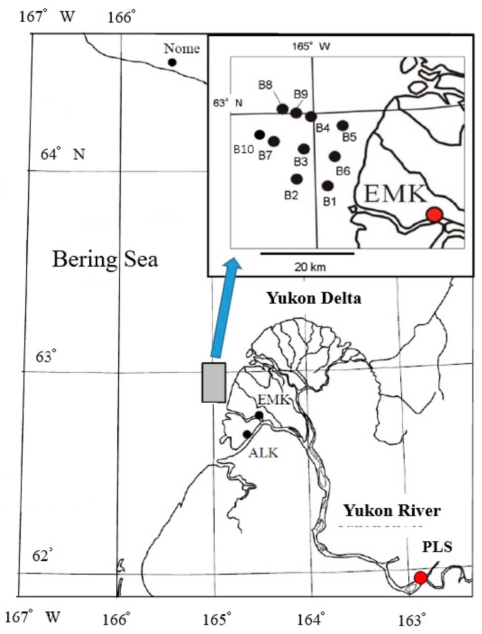
2. Study Area
3. Methods
3.1. Field Observations
3.2. Laboratory Experiments
4. Results
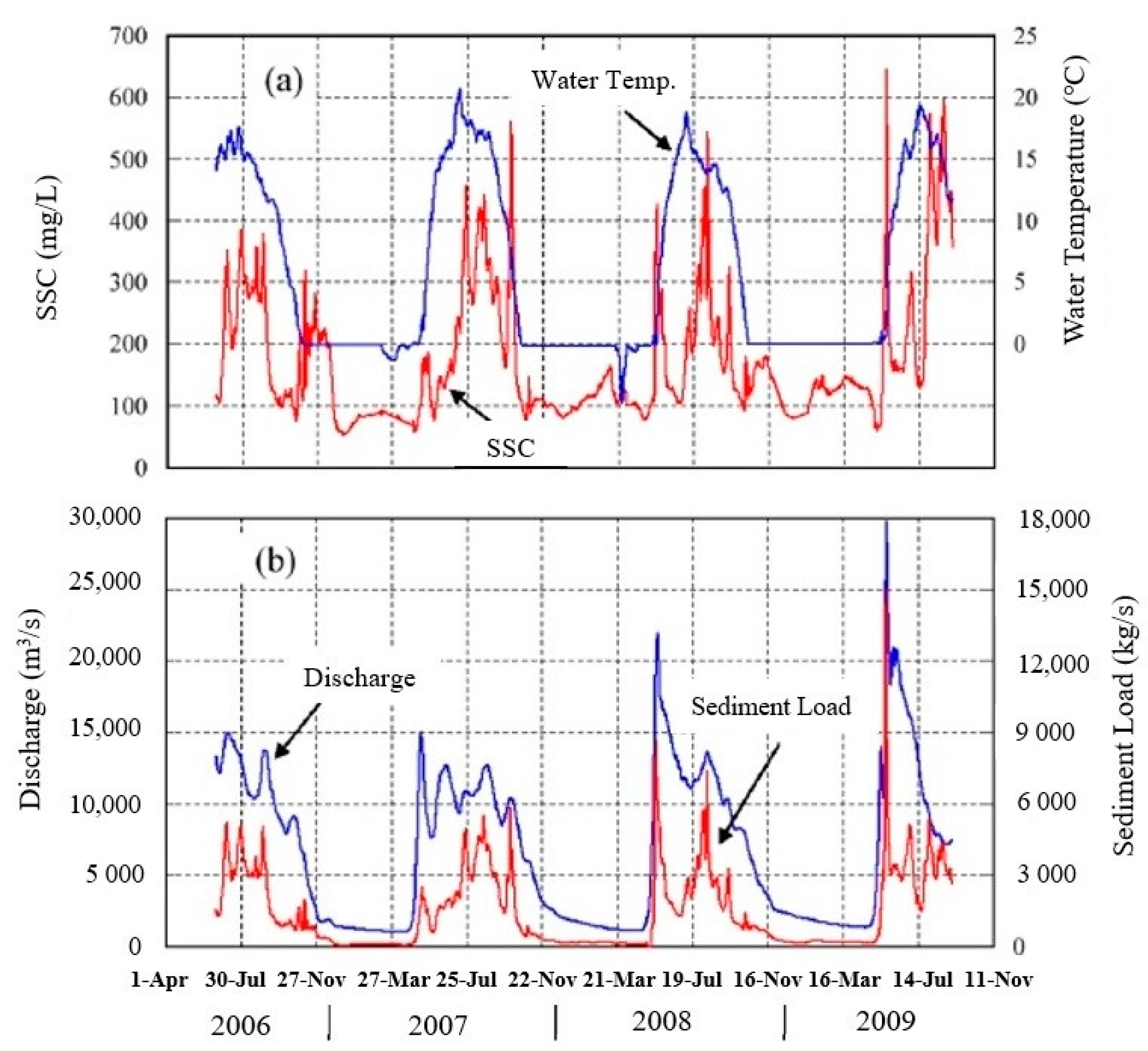
4.1. Time Series of Discharge and Sediment Load
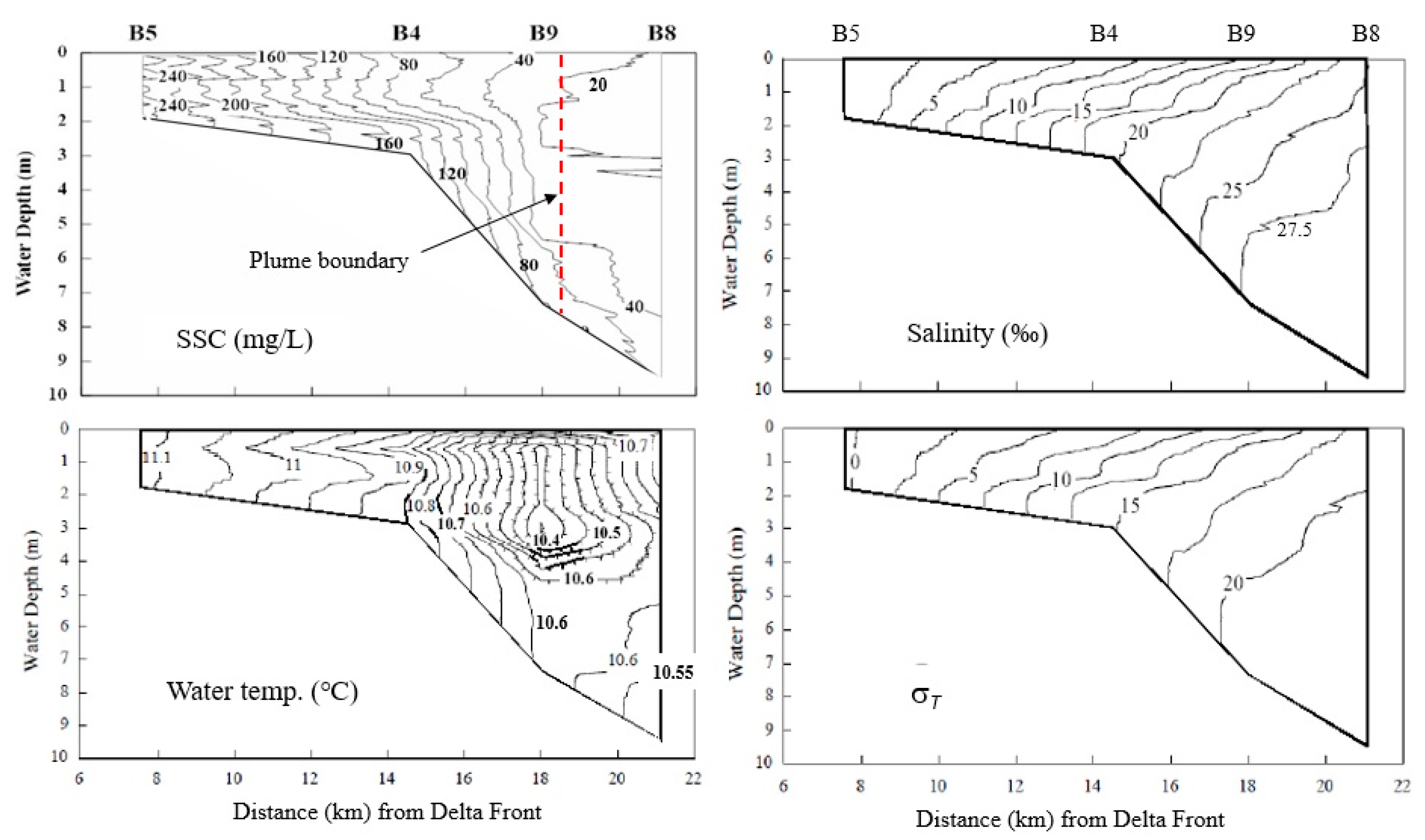
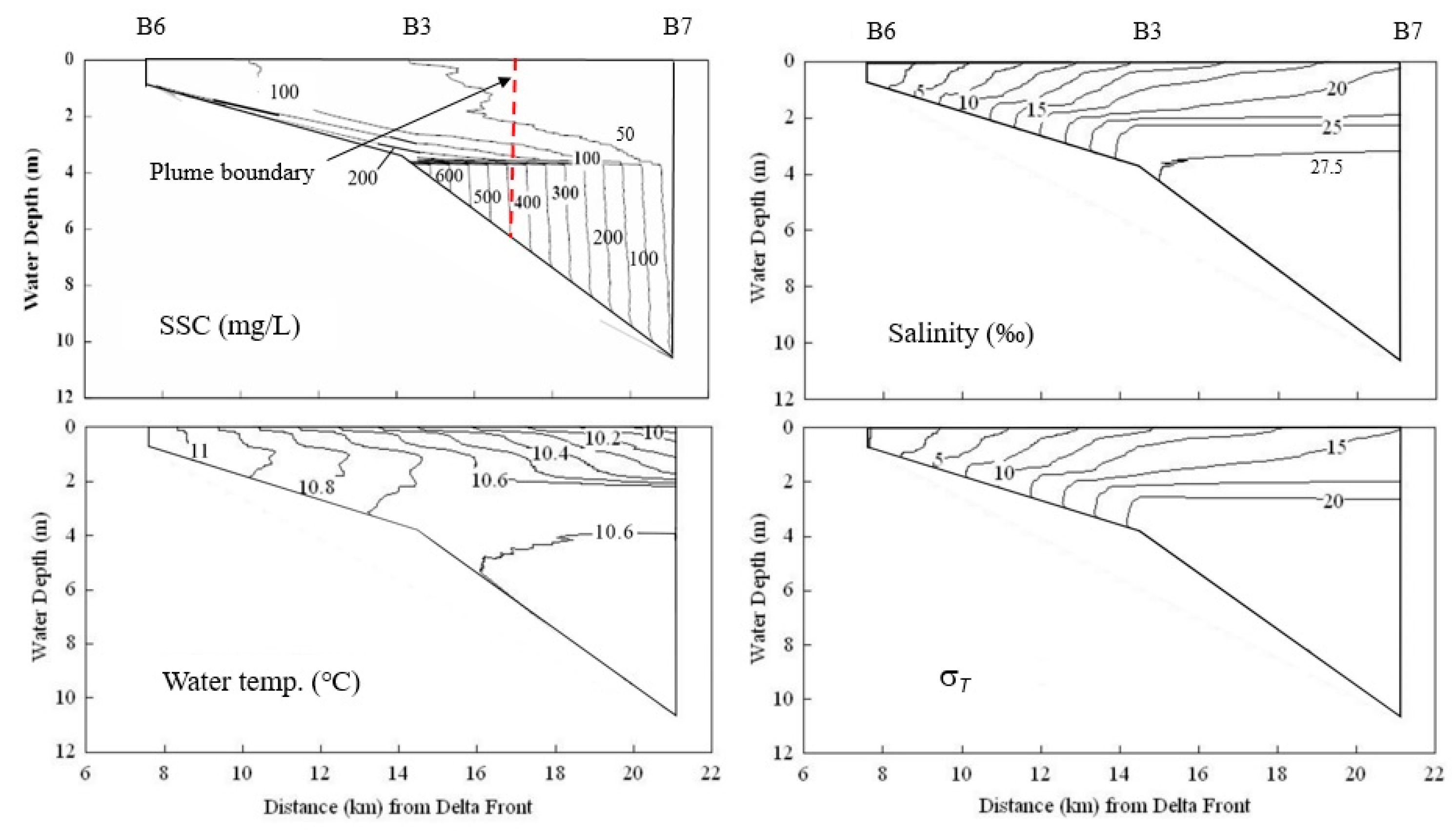
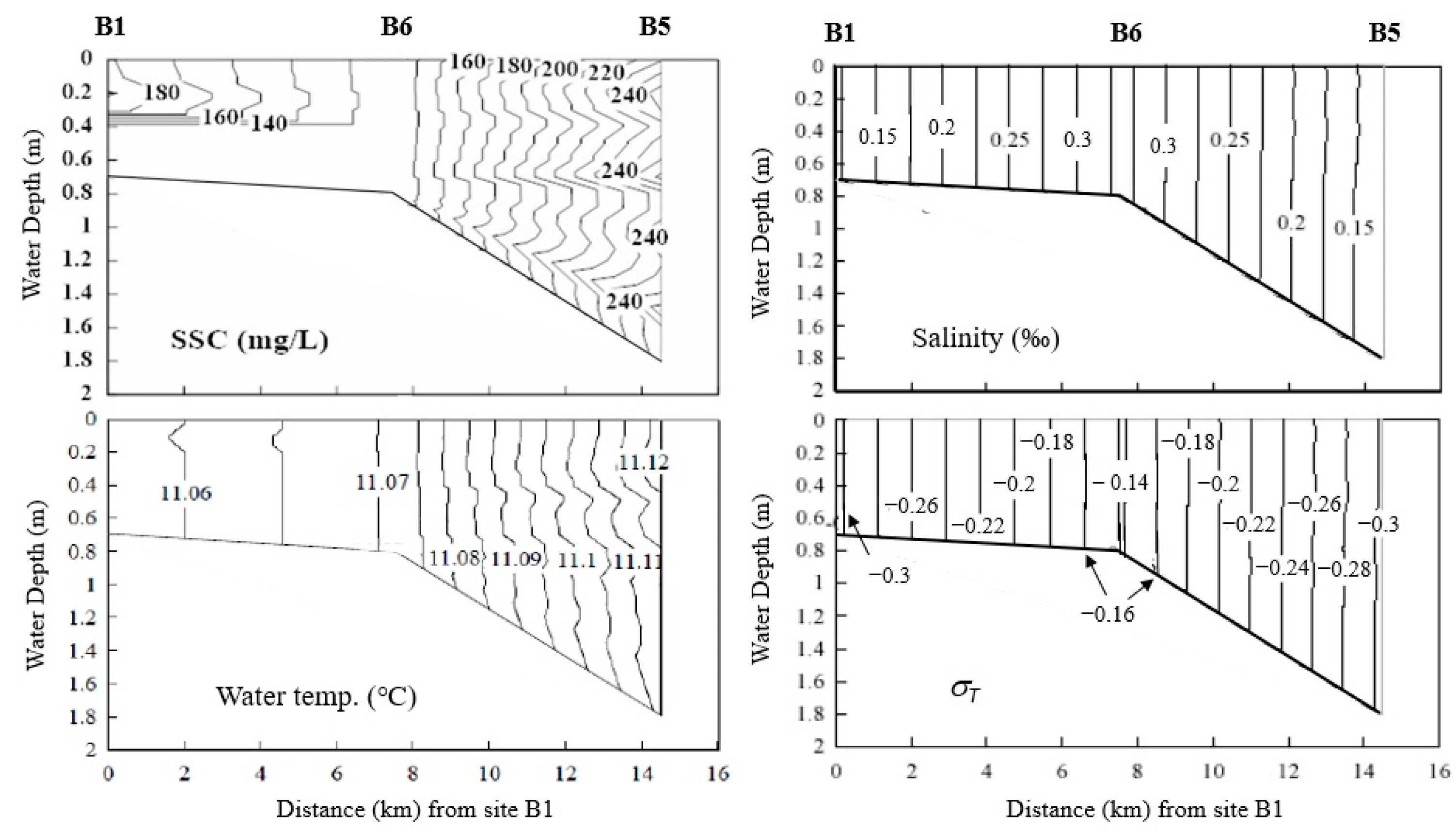
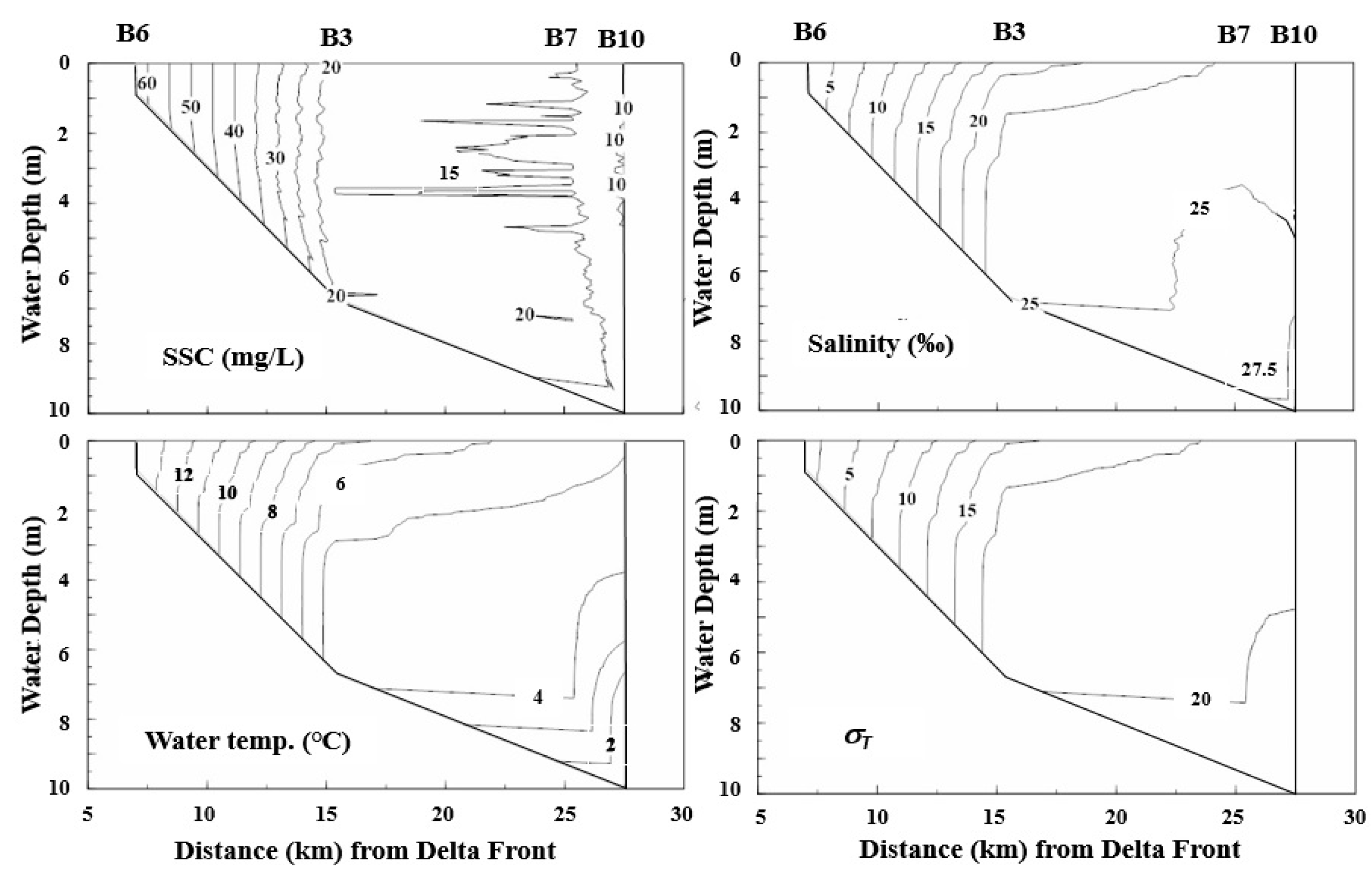
4.2. Observational Results of Plume Behaviors
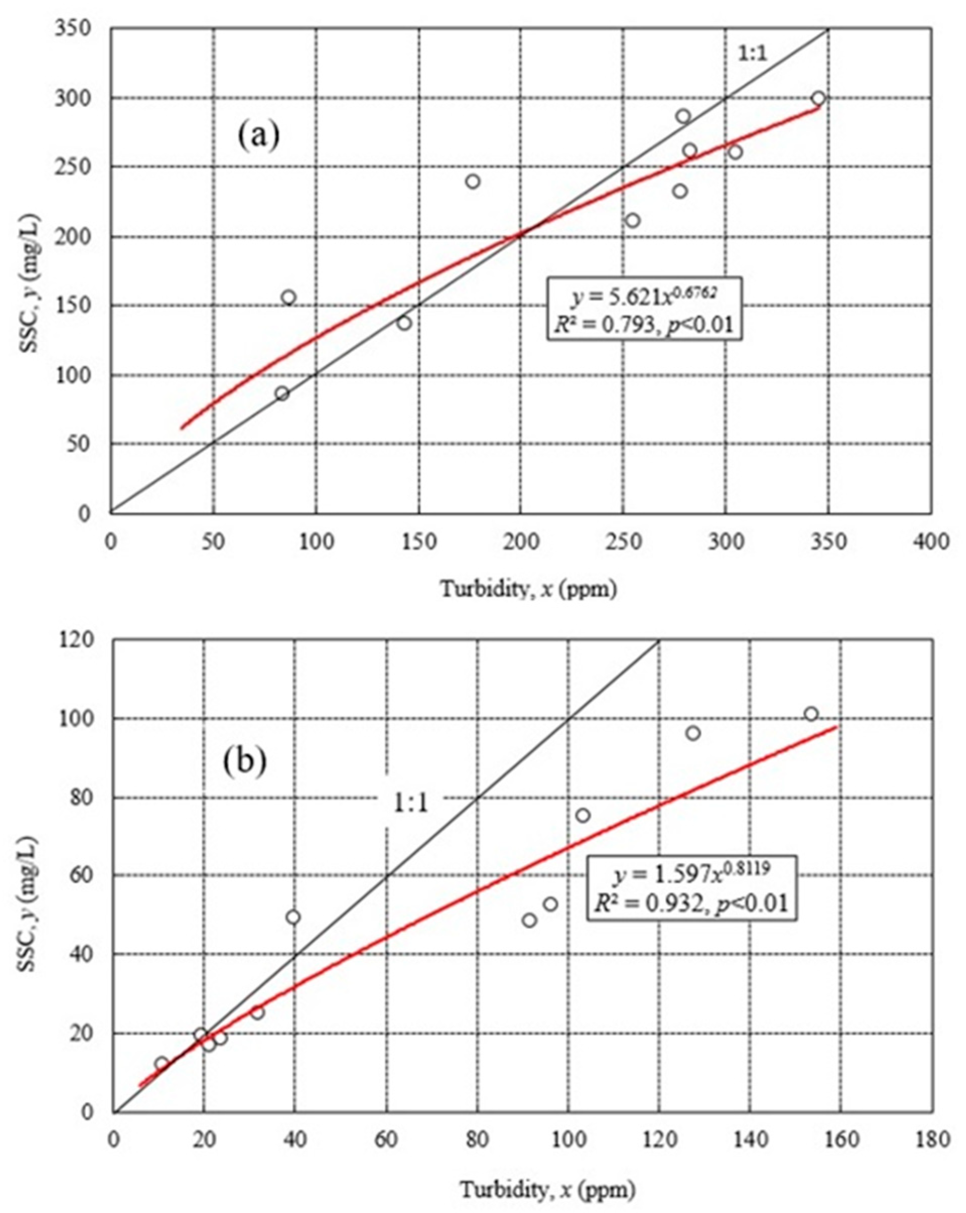
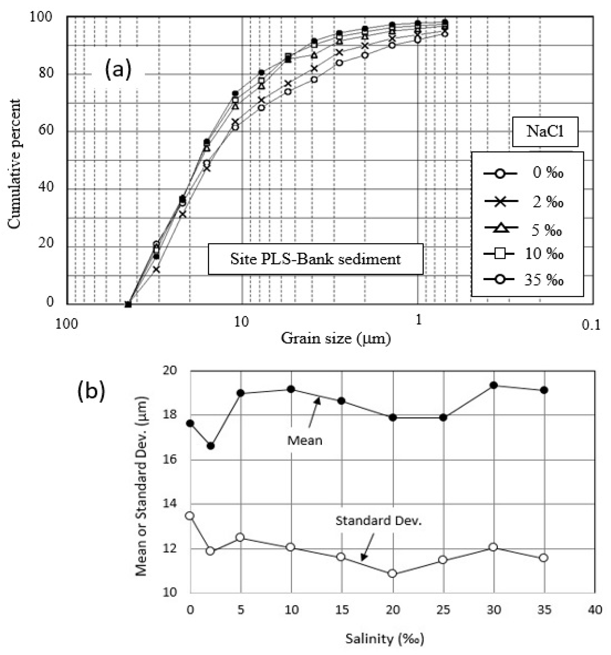
4.3. Experimental Results for Yukon Sediment
5. Discussion
6. Conclusions
Author Contributions
Funding
Acknowledgments
Conflicts of Interest
References
- Milligan, T.G.; Hill, P.S.; Law, B.A. Flocculation and the loss of sediment from the Po River plume. Cont. Shelf Res. 2007, 27, 309–321. [Google Scholar] [CrossRef]
- Strom, K.; Keyvani, A. Flocculation in a decaying shear field and its implications for mud removal in near-field river mouth discharges. J. Geophys. Res. Oceans 2016, 121, 2142–2162. [Google Scholar] [CrossRef]
- Hetland, R.; Hsu, T. Freshwater and sediment dispersal in large river plumes. In Biogeochemical Dynamics at Major River-Coastal Interfaces: Linkages with Global Change; Bianchi, T., Allison, M., Cai, W., Eds.; Cambridge University Press: Cambridge, UK, 2013; pp. 55–85. [Google Scholar] [CrossRef]
- Markussen, T.N.; Elberling, B.; Winter, C.; Andersen, T.J. Flocculated meltwater particles control Arctic land-sea fluxes of labile iron. Sci. Rep. 2016, 6, 24033. [Google Scholar] [CrossRef] [PubMed]
- Milligan, R.P.; Perrie, W.; Solomon, S. Dynamics of the Mackenzie River plume on the inner Beaufort shelf during an open water period in summer. Estuar. Coast. Shelf Sci. 2010, 89, 214–220. [Google Scholar] [CrossRef]
- Qiao, S.; Shi, X.; Zhu, A.; Liu, Y.; Bi, N.; Fang, X.; Yang, G. Distribution and transport of suspended sediments off the Yellow River (Huanghe) mouth and the nearby Bohai Sea. Estuar. Coast. Shelf Sci. 2010, 86, 337–344. [Google Scholar] [CrossRef]
- Wang, H.; Bi, N.; Wang, Y.; Saito, Y.; Yang, Z. Tide-modulated hyperpycnal flows off the Huanghe (Yellow River) mouth, China. Earth Surf. Process. Landf. 2010, 35, 1315–1329. [Google Scholar] [CrossRef]
- Pan, J.; Gu, Y.; Wang, D. Observations and numerical modeling of the Pearl River plume in summer season. J. Geophys. Res. Oceans 2014, 119, 2480–2500. [Google Scholar] [CrossRef]
- Saldıas, G.; Shearman, R.K.; Barth, J.A.; Tufillaro, N. Optics of the offshore Columbia River plume from glider observations and satellite imagery. J. Geophys. Res. Oceans 2016, 121, 2367–2384. [Google Scholar] [CrossRef] [Green Version]
- Cole, K.L.; Hetland, R.D. The effects of rotation and river discharge on net mixing in small-mouth Kelvin number plumes. J. Phys. Oceanogr. 2016, 46, 1421–1436. [Google Scholar] [CrossRef]
- Varona, H.L.; Veleda, D.; Silva, M.; Cintra, M.; Araujo, M. Amazon River plume influence on Western Tropical Atlantic dynamic variability. Dyn. Atmos. Oceans 2019, 85, 1–15. [Google Scholar] [CrossRef]
- Gouveia, N.A.; Gherardi, D.F.M.; Aragão, L.E.O.C. The role of the Amazon River plume on the intensification of the hydrological cycle. Geophys. Res. Lett. 2019, 46, 12221–12229. [Google Scholar] [CrossRef]
- de Oliveira, E.N.; Knoppers, B.A.; Lorenzzetti, J.A.; Medeiros, P.R.P.; Carneiro, M.E.; de Souza, W.F.L. A satellite view of riverine turbidity plumes on the NE-E Brazilian coastal zone. Braz. J. Oceanogr. 2012, 60, 283–298. [Google Scholar] [CrossRef] [Green Version]
- Restrepo, J.D.; Park, E.; Aquino, S.; Latrubesse, E.M. Coral reefs chronically exposed to river sediment plumes in the southwestern Caribbean: Rosario Islands, Colombia. Sci. Total Environ. 2016, 553, 316–329. [Google Scholar] [CrossRef]
- Dean, K.G.; McRoy, C.P.; Ahlnäs, K.; Springer, A. The plume of the Yukon River in relation to the Oceanography of the Bering Sea. Remote Sens. Environ. 1989, 28, 75–84. [Google Scholar] [CrossRef]
- Pitarch, J.; Falcini, F.; Nardin, W.; Brando, V.E.; Di Cicco, A.; Marullo, S. Linking flow-stream variability to grain size distribution of suspended sediment from a satellite-based analysis of the Tiber River plume (Tyrrhenian Sea). Sci. Rep. 2016, 9, 19729. [Google Scholar] [CrossRef]
- Brabets, T.P.; Wang, B.; Meade, R.H. Environmental and Hydrologic Overview of the Yukon River Basin, Alaska and Canada; Water-Resources Investigations Report; U. S. Geological Survey: Anchorage, AK, USA, 2000. [CrossRef]
- Striegl, R.G.; Dornblaser, M.M.; Aiken, G.R.; Wickland, K.P.; Raymond, P.A. Carbon export and cycling by the Yukon, Tanana, and Porcupine Rivers, Alaska, 2001–2005. Water Resour. Res. 2007, 43, W02411. [Google Scholar] [CrossRef] [Green Version]
- Chikita, K.A.; Wada, T.; Kudo, I.; Kim, Y. The intra-annual variability of discharge, sediment load and chemical flux from the monitoring: The Yukon River, Alaska. J. Water Resour. Prot. 2012, 4, 173–179. [Google Scholar] [CrossRef] [Green Version]
- Chikita, K.A.; Wada, T.; Kudo, I. Material-loading processes in the Yukon River basin, Alaska: Observations and modelling. Low Temp. Sci. 2016, 74, 43–54. [Google Scholar] [CrossRef]
- Nelson, H.; Creager, J.S. Displacement of Yukon-derived sediment from Bering Sea to Chukchi Sea during Holocene time. Geology 1977, 5, 141–146. [Google Scholar] [CrossRef]
- Ortiz, J.D.; Polyak, L.; Grebmeier, J.M.; Darby, D.; Eberl, D.D.; Naidu, S.; Nof, D. Provenance of Holocene sediment on the Chukchi-Alaskan margin based on combined diffuse spectral reflectance and quantitative X-ray diffraction analysis. Glob. Planet. Chang. 2009, 68, 73–84. [Google Scholar] [CrossRef]
- Chikita, K.A.; Kemnitz, R.; Kumai, R. Characteristics of sediment discharge in the subarctic Yukon River, Alaska. Catena 2002, 48, 235–253. [Google Scholar] [CrossRef]
- Chikita, K. A field study on turbidity current initiated from spring runoffs. Water Resour. Res. 1989, 25, 257–271. [Google Scholar] [CrossRef]
- Chikita, K. Sedimentation by river-induced turbidity currents: Field measurements and interpretation. Sedimentology 1990, 37, 891–905. [Google Scholar] [CrossRef]
- Knoblauch, H. Overview of Density Flows and Turbidity Currents; Water Resources Research Laboratory, U.S. Bureau of Reclamation: Denver, CO, USA, 1999; pp. 1–27.
- Whitehouse, U.G.; James, L.M.; Debbrecht, J.D. Differential settling tendencies of clay minerals in saline waters. Clays Clay Miner. 1958, 7, 1–79. [Google Scholar] [CrossRef]
- Lick, W.; Huang, H.; Jepsen, R. Flocculation of fine-grained sediments due to differential settling. J. Geophys. Res. Oceans 1993, 98, 10279–10288. [Google Scholar] [CrossRef]


Publisher’s Note: MDPI stays neutral with regard to jurisdictional claims in published maps and institutional affiliations. |
© 2021 by the authors. Licensee MDPI, Basel, Switzerland. This article is an open access article distributed under the terms and conditions of the Creative Commons Attribution (CC BY) license (http://creativecommons.org/licenses/by/4.0/).
Share and Cite
Chikita, K.A.; Wada, T.; Kudo, I.; Saitoh, S.-I.; Toratani, M. Effects of River Discharge and Sediment Load on Sediment Plume Behaviors in a Coastal Region: The Yukon River, Alaska and the Bering Sea. Hydrology 2021, 8, 45. https://0-doi-org.brum.beds.ac.uk/10.3390/hydrology8010045
Chikita KA, Wada T, Kudo I, Saitoh S-I, Toratani M. Effects of River Discharge and Sediment Load on Sediment Plume Behaviors in a Coastal Region: The Yukon River, Alaska and the Bering Sea. Hydrology. 2021; 8(1):45. https://0-doi-org.brum.beds.ac.uk/10.3390/hydrology8010045
Chicago/Turabian StyleChikita, Kazuhisa A., Tomoyuki Wada, Isao Kudo, Sei-Ichi Saitoh, and Mitsuhiro Toratani. 2021. "Effects of River Discharge and Sediment Load on Sediment Plume Behaviors in a Coastal Region: The Yukon River, Alaska and the Bering Sea" Hydrology 8, no. 1: 45. https://0-doi-org.brum.beds.ac.uk/10.3390/hydrology8010045