
Predicting Urban Flooding Due to Extreme Precipitation Using a Long Short-Term Memory Neural Network


Water Engineering and Management Department, University of Twente, 7500 AE Enschede, The Netherlands
*
Author to whom correspondence should be addressed.
Hydrology 2022, 9(6), 105; https://0-doi-org.brum.beds.ac.uk/10.3390/hydrology9060105
Submission received: 6 May 2022
/
Revised: 2 June 2022
/
Accepted: 6 June 2022
/
Published: 10 June 2022
(This article belongs to the Special Issue Modern Developments in Flood Modelling)
Abstract
:Extreme precipitation events can lead to the exceedance of the sewer capacity in urban areas. To mitigate the effects of urban flooding, a model is required that is capable of predicting flood timing and volumes based on precipitation forecasts while computational times are significantly low. In this study, a long short-term memory (LSTM) neural network is set up to predict flood time series at 230 manhole locations present in the sewer system. For the first time, an LSTM is applied to such a large sewer system while a wide variety of synthetic precipitation events in terms of precipitation intensities and patterns are also captured in the training procedure. Even though the LSTM was trained using synthetic precipitation events, it was found that the LSTM also predicts the flood timing and flood volumes of the large number of manholes accurately for historic precipitation events. The LSTM was able to reduce forecasting times to the order of milliseconds, showing the applicability of using the trained LSTM as an early flood-warning system in urban areas.
1. Introduction
Extreme precipitation events, of both short and long duration, can cause inundations locally or downstream of a catchment due to raising river water levels [1]. This research focuses on local flooding due to extreme precipitation events and more specifically on urban flooding due to the exceedance of the sewer capacity. Pluvial urban flooding can occur quite suddenly, and therefor, early flood warning systems with a short run time are desired such that proper flood mitigation measures can be taken in time. Urban flooding differs from flooding in other areas because of the large amount of impervious surface area negating infiltration and increasing the load on sewer systems. Flooding in an urban environment is caused by short extreme precipitation events where infiltration is negligible. It is expected that flood probabilities will increase in the future due to an increase in impervious surface area, causing more runoff to the sewer system. In addition, due to climate change, it is expected that rainfall intensities will increase locally, resulting in higher runoff volumes [2,3].
Numerical models are generally used to investigate the effects of extreme precipitation events on inundation extents and to design sewer systems accordingly. These physics-based models are computationally expensive. Since precipitation forecasts are generally highly uncertain, especially for extreme local events, a probabilistic approach is required to simulate all potential flood scenarios. Consequently, detailed physics-based models cannot be used as a flood early warning systems. However, a fast prediction of the inundated areas during extreme events ensures that flood mitigation measures can be taken on time. For this reason, other approaches for the faster computation of flood predictions have been studied in recent years (e.g., [4,5]). A commonly applied method to reduce computational load is surrogate modelling, representing a second-level abstraction from the original system. Response surface surrogate models, such as machine learning (ML) algorithms, are data-driven models trained based on the input–output relations of a physically based model or field measurements. As a result, ML algorithms do not capture any physical components of the original system. They are, once trained, extremely fast in predicting the output based on a given input [6] and can do so on a continuous basis. For this reason, ML algorithms have frequently been applied for water resources applications [6,7]. More specifically, many studies have already shown the applicability of ML algorithms to predict (historic) stream flow conditions, weather conditions, water quality and dike breaches accurately (e.g., [8,9,10,11,12,13]). However, the use of ML algorithms for sewer applications is still limited, but they have great possibilities in predicting sewer overflows based on precipitation forecasts.
Recent examples of ML algorithms for sewer system applications are presented by [14,15]. Rjeily et al. [14] developed a data-driven modelling approach to predict water depth variations within the most critical manholes in an urban drainage system. This early flood warning system was trained using measurements of 10 storm events simulated with a hydraulic model. Measured rainfall intensities and modelled water depth variations in five manholes were used as the input and target output data, respectively. Zang et al. [15] studied the accuracy of multiple ML algorithms to predict sewer overflow of a combined sewer system into open water bodies causing heavy pollution. In total, 26 rainfall events resulting in sewer overflow were used to train the various ML algorithms. Although both studies showed the potential of using ML algorithms as an early warning system for sewer applications, these studies only used a few historic events to train the algorithms, while using more samples can ensure better model performance since it is more likely that the global minimum of the error function is found [16]. Therefore, it is questionable if the trained the ML algorithms are able to generalise the system behaviour. Furthermore, because of expected climate change, more extreme precipitation events may occur than observed so far, but these events are not considered in the training data sets if historic events are considered. Therefore, a synthetic data set with a wide variety of rainfall events in terms of both rainfall intensities and rainfall patterns will be used in this study. Additionally, the studies conducted so far only predicted sewer overflow at a few predefined output locations while an overview of the entire sewer system is required to make fair flood mitigation measures during extreme events. For this reason, the objective of this research is to set up an ML algorithm that predicts flood volume time series for all manholes present in a specific urban area, trained on a wide variety of rainfall events. Only then will the developed ML algorithm have the potential to be used as an early flood warning system by decision makers.
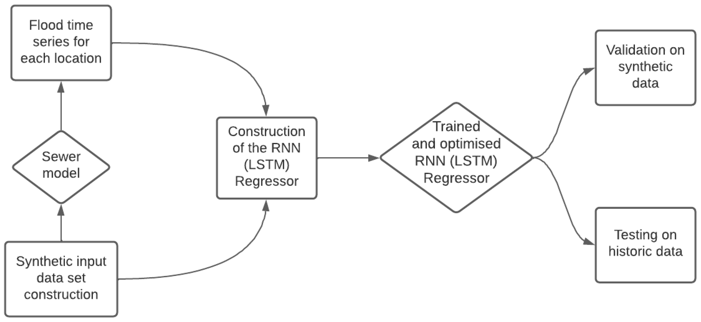
The methodology of this research is shown in Figure 1. First, the case study and the numerical sewer model used to create the training data are described (Section 2). A synthetic precipitation data set is constructed since no sufficient historic rainfall events resulting in flood inundations exist and to enable the inclusion of a wider variety of precipitation events than observed so far (Section 3). These synthetic rainfall events are used as input of the numerical sewer model. An ML algorithm is constructed which is able to predict flood volume time series for all manholes in the area as the target output, given a precipitation time series as input (Section 4). The constructed ML algorithm is validated to determine the final performance of the algorithm (Section 5.1). Furthermore, the algorithm is tested based on radar rainfall measurements of a few historic extreme precipitation events (Section 5.2). This paper ends with a discussion (Section 6) and the main conclusions (Section 7).
2. Case Study and the Numerical Sewer Model
The residential area of Hooglanderveen in the city of Amersfoort, the Netherlands, is chosen as a case study since frequent pluvial flooding occurs in this region. Although the region of Hooglanderveen is chosen as a case study, the proposed methods in this study are applicable to any residential area with a similar sewer system and topographical features.
Hooglanderveen is located in the northeast of Amersfoort (see Figure 2) and has a surface area of approximately 1.75 km2.
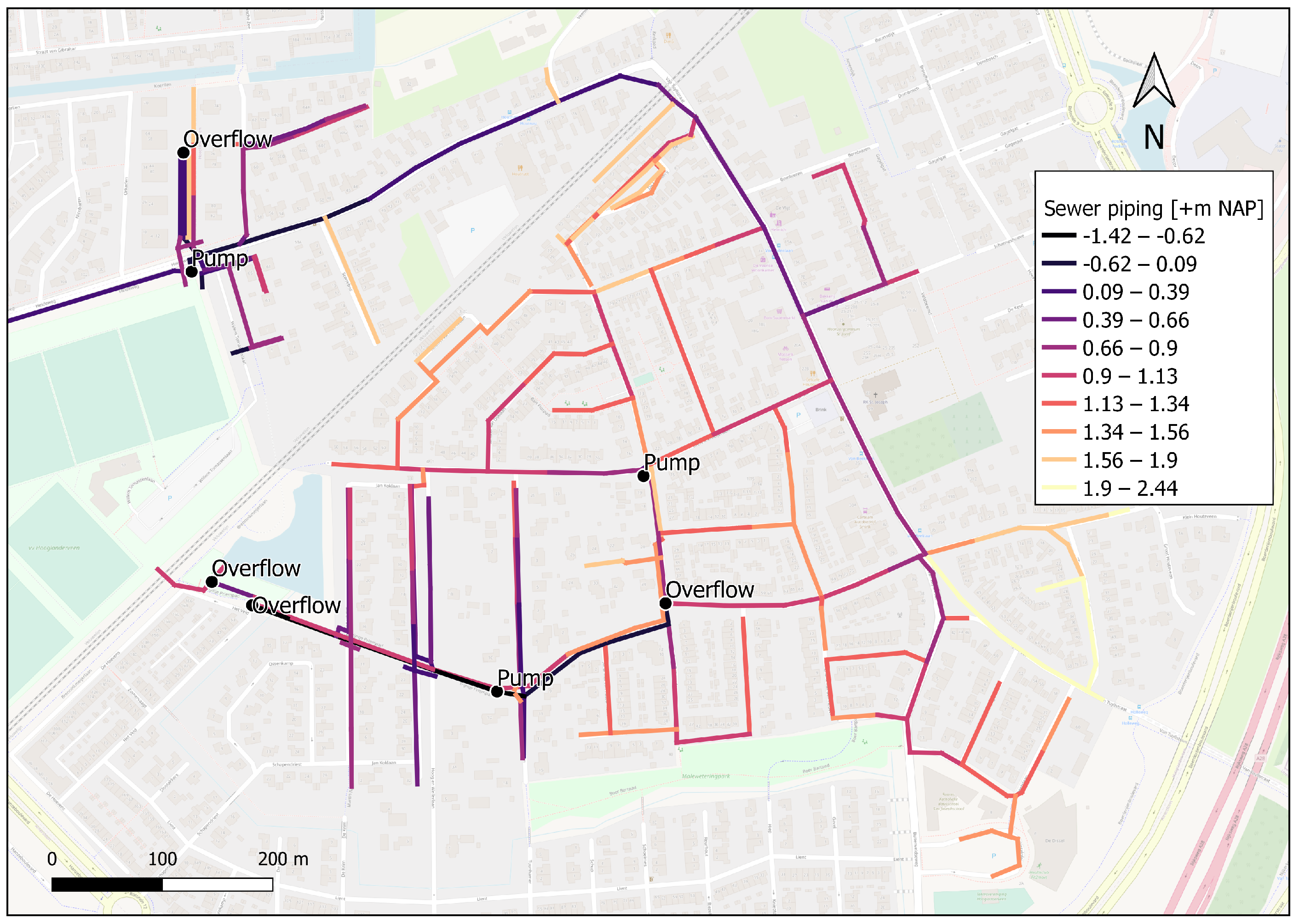
Especially in the northwestern region of Hooglanderveen, frequent pluvial flooding is experienced, where surface levels are relatively low. The combined sewer system present in Hooglanderveen is a type of gravity sewer and has 230 manholes, 4 pumps, and 3 overflows (Figure 3). These are all connected with sewer pipes (Figure 3). The sewer system transports both precipitation runoff and domestic sewage to a sewage treatment plant and can be divided into two components: (1) the major sewer system, consisting of streets, inlets, ditches, and surface water channels, and (2) the minor sewer system, composed of interconnected pipes, manholes, and pumps [1]. The major system can be characterised as the surface system, whereas the minor system represents the subsurface system. Flooding occurs whenever and wherever the discharge capacity of the inlet into the minor system is exceeded. This can have several causes. First, flooding can occur when precipitation intensity exceeds the discharge capacity of the inlet. Water cannot enter the minor system and remains at the surface level. Second, the discharge capacity may be lower between some sewer pipes due to, e.g., clogging or smaller pipe diameters causing water to flow back onto the streets through the inlets or manholes. Third, the combined gravity-driven sewer system has a larger discharge capacity than the pump at the end of the system. Therefore, a storage is designed in the minor system to accommodate this difference in capacity. This storage is equivalent to approximately 7–9 mm of precipitation in the Netherlands [17]. When the storage capacity is exceeded and more water enters the system, storm water will exit via the overflows. If the capacity of the overflows is exceeded, storm water will flood the streets.
In this study, an ML algorithm is set up to predict flooding in Hooglanderveen in real-time precipitation forecasts. An ML algorithm is generally trained using field measurements based on historical events or outcomes of model simulations. Since insufficient measurements are available of historic precipitation events resulting in flooding in the study area, a numerical sewer model will be used to generate the training data. The numerical sewer model is a validated model built with the software Infoworks ICM. The sewer model represents a one-dimensional (1D) model of the minor system and uses the shallow water equations to solve the 1D flow. Only the surface area of the major system, without considering topographic gradients, is included in the model. Based on these areas, the shortest flow paths to the nearest inlet is determined to compute the inflow from the major system into the minor system. Henonin et al. [18] further details the modelling approach of such a 1D sewer model. The sewer model was calibrated using measurements and is used by local ministries for flood risk evaluation.
The sewer system has a slope from the southeastern to northwestern part of the study area. Since it is a gravity-based sewer system, the general direction of the sewer flow follows this slope. The model has as input a spatially uniform precipitation event and provides as output flood volumes at each manhole in the area. Note that the output is a flood volume and not a flood level, as topographic gradients of the surface level and the flow along these topographic gradients are not included in the model.
3. Training and Testing Data
3.1. The Synthetic Precipitation Events
The sewer model computes flood volumes based on an input precipitation event. In this study, synthetic events are considered to enable the inclusion of a wide variety of precipitation events. These synthetic precipitation events are based on design events to test the sewer systems using numerical models in the Netherlands [19]. Spatially uniform precipitation events are considered because of the relatively small size of the studied area. For the construction of the synthetic precipitation training data set, statistics of the following three precipitation characteristics are used [19]: precipitation duration, precipitation intensity, and precipitation pattern. Combinations between the three characteristics are made to generate unique precipitation events.
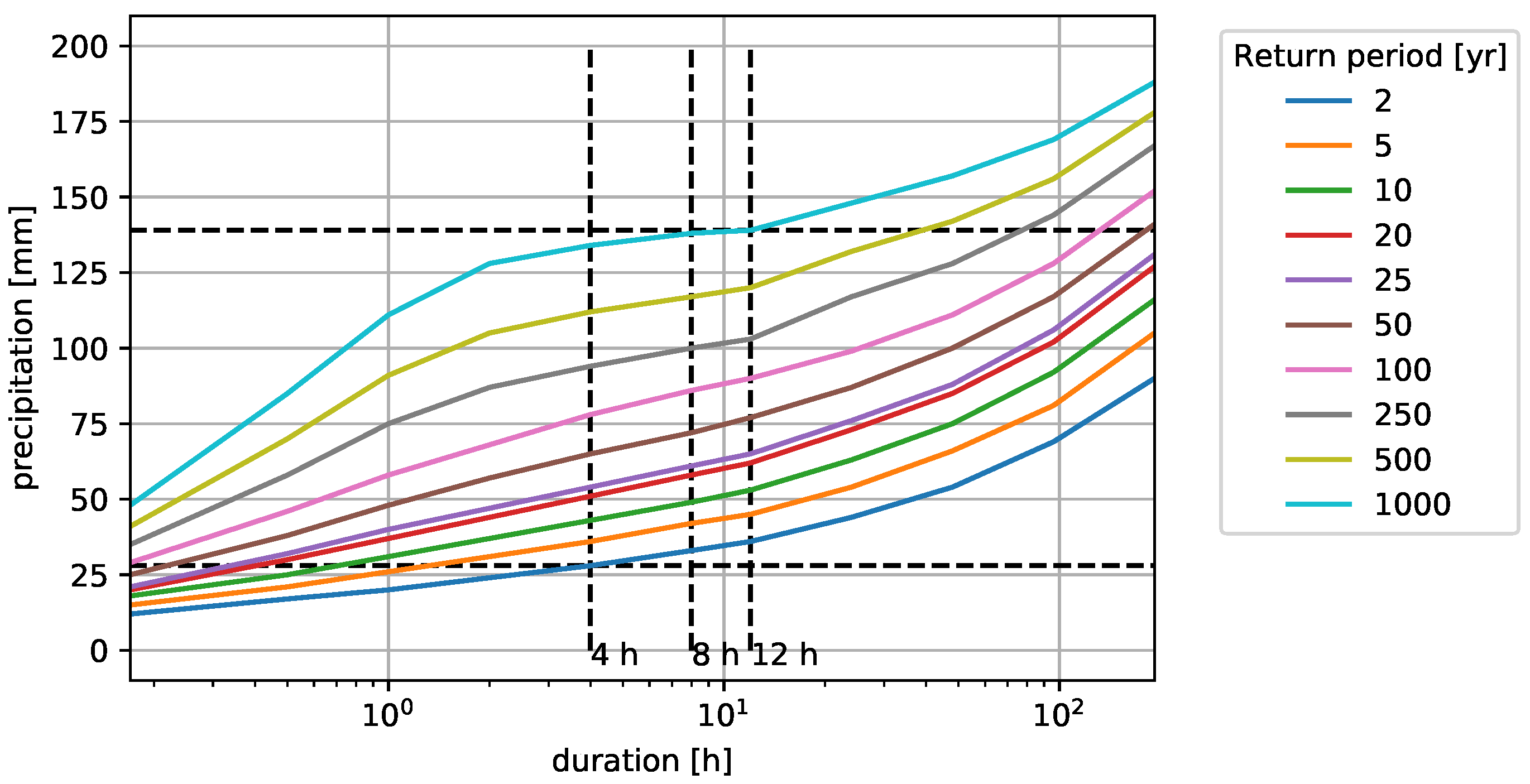
Due to the inherent early warning system that is proposed in the present research, we focus on short-term, high-intensity flood events. For this, [19] recommends a precipitation duration of 4, 8, or 12 h. The minimum and maximum precipitation intensities corresponding to a return period of 2 to 1000 years for a duration of 4 and 12 h are 28 mm and 139 mm, respectively (Figure 4 shows the intensity curves for a return period of 2 to 1000 years). To generate the training data set, the precipitation intensities are divided into six values with a minimum and maximum of 30 mm and 105 mm, respectively. The minimum value is taken as the rounded minimum value given by the precipitation curves (Figure 4). The maximum value is set to a lower value than provided by the precipitation curves since increasing the intensity to a value larger than 105 mm did not result in any differences in model output in terms of flood complexity since the number of flooded manholes remained constant. Only the flood volumes increased linearly.
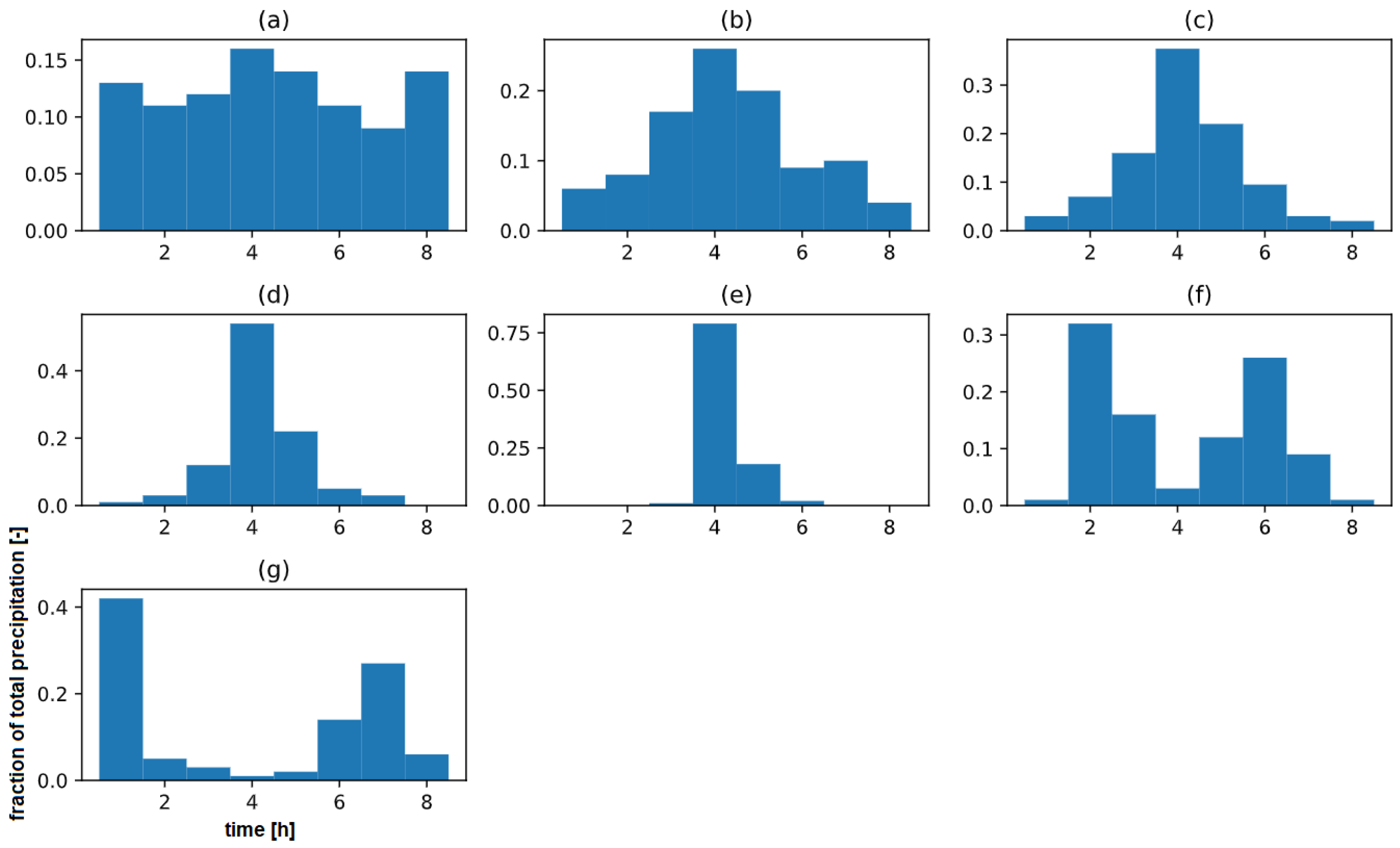
In addition to the precipitation duration and intensity, seven distinct precipitation patterns for short-term events are considered in the Dutch water policy [19]. These patterns consist of a fraction of the total precipitation per hour. The seven precipitation patterns can be described as follows (Figure 5):
- Uniform: General uniform shape with minor changes in precipitation intensity during the event;
- One peak—: Pattern with one peak that has of the total intensity in the peak;
- One peak—: Pattern with one peak that has of the total intensity in the peak;
- One peak—: Pattern with one peak that has of the total intensity in the peak;
- One peak—: Pattern with one peak that has of the total intensity in the peak;
- Two peaks—short distance: Pattern with two peaks that has a small temporal distance between the two peaks;
- Two peaks—large distance: Pattern with two peaks that has a large temporal distance between the two peaks;
With six precipitation intensity values, seven precipitation patterns, and three precipitation durations, the total amount of unique precipitation events is 126. The majority of papers reviewed by [16] use a minimum data set size of 100 samples to train the ML algorithms, indicating that the size of the data set should be sufficiently large to train the ML algorithm properly. All possible values of each precipitation feature are shown in Table 1.
3.2. Interpolation of Precipitation Patterns
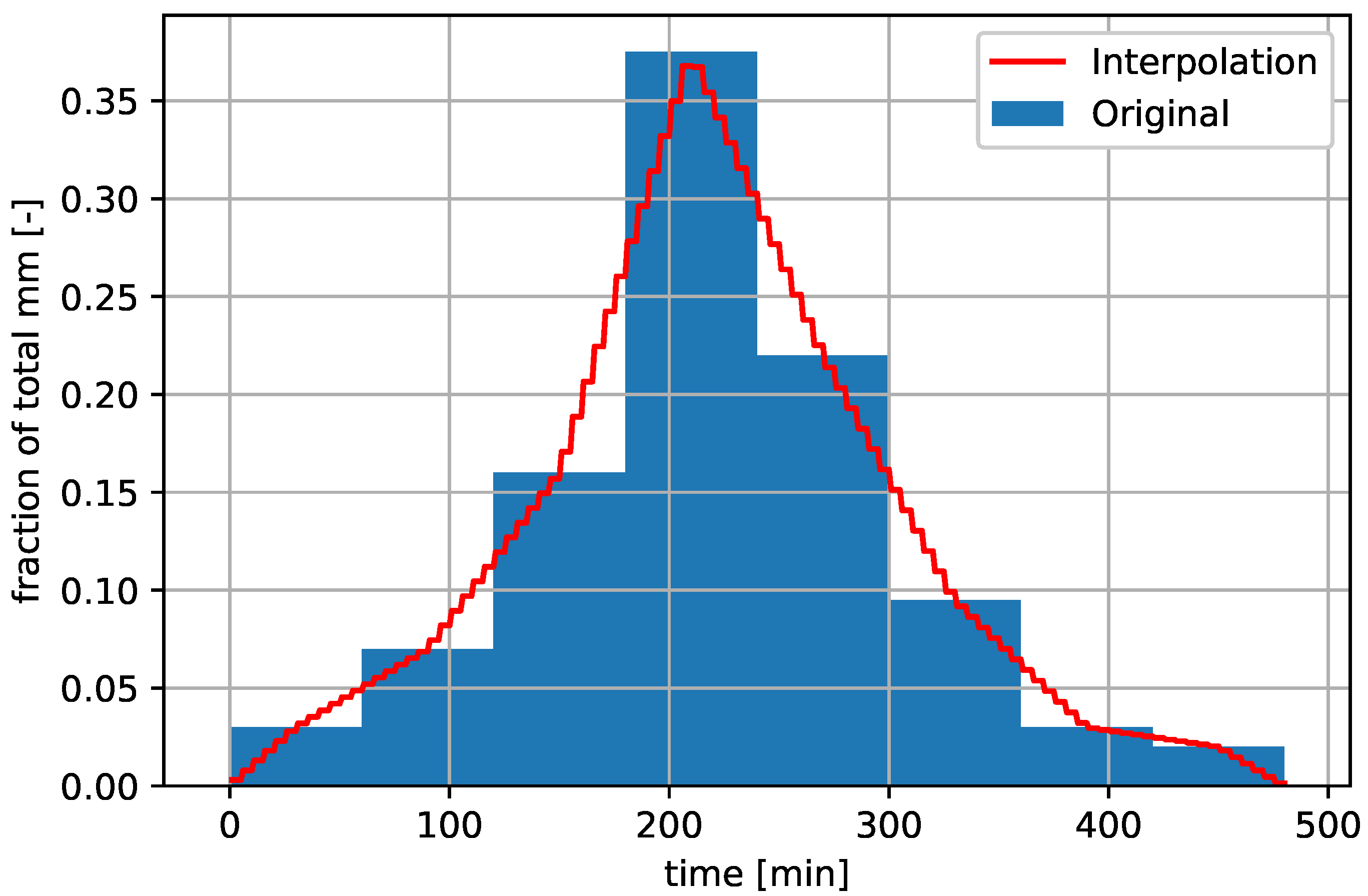
The precipitation patterns provided by [19] have a time step of one hour, while the time step of the sewer model is set to one minute to ensure accurate model results. For this reason, the precipitation patterns are linearly interpolated to create realistic precipitation events. Furthermore, to facilitate the operationally of a flood early warning system, the input time series is made to mimic a conventional precipitation forecast. Based on expert opinion, it was found that for short-term precipitation forecasts, a time step of 5 min is generally used. Therefore, the input time series will be a cascading precipitation pattern with a time step of 1 min, which changes its value after every 5 min (Figure 6). Due to this interpolation method, the total precipitation is, at maximum, 2% lower than the value as defined.
3.3. Historic Data
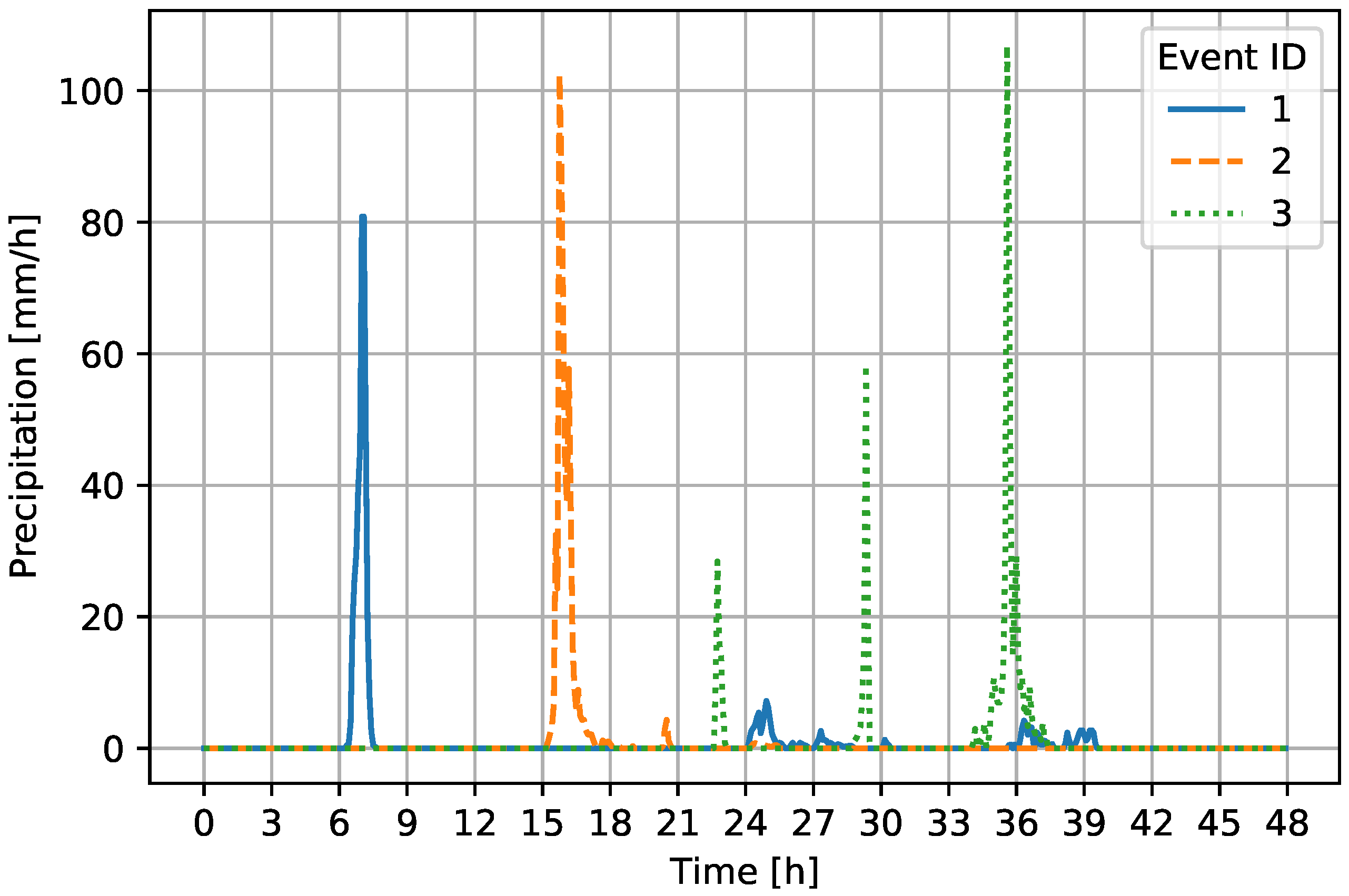
The synthetic data set is used to train, validate, and test the LSTM. However, this raises the question whether the LSTM, trained on synthetic data, is capable of reproducing the results of the sewer model on real-world precipitation data. To evaluate this, radar precipitation data from historic extreme precipitation events were obtained. A list of three reported flood events in Hooglanderveen was provided by the municipality of Amersfoort, and related precipitation time series were obtained from precipitation radar data provided by Hydrologic (Figure 7) and used as input for the sewer model. The time series start one day prior to the date that a flood was reported, as there can be a delay between flooding and reporting. All events show large peaks in precipitation up to 106 mm/h. This precipitation peak is higher than the value used in the synthetic data set, having a maximum precipitation of 88 mm/h.
4. Construction of the Long Short-Term Memory (LSTM) Neural Network
In this study, the LSTM neural network proposed by [20] is used to predict flood volumes for the 230 manholes in the sewer system of Hooglanderveen. Although many neural network structures exist, LSTMs have shown to be most successful and are generally applied to predict time series [21]. More specifically, LSTM has become the focus of deep learning because of their powerful learning capacity in comparison to other recurrent neural network (RNN) approaches [21]. To explain the concept of an LSTM, we first briefly explain artificial neural networks (ANN) and recurrent neural networks (RNN).
4.1. The Concept of Neural Networks
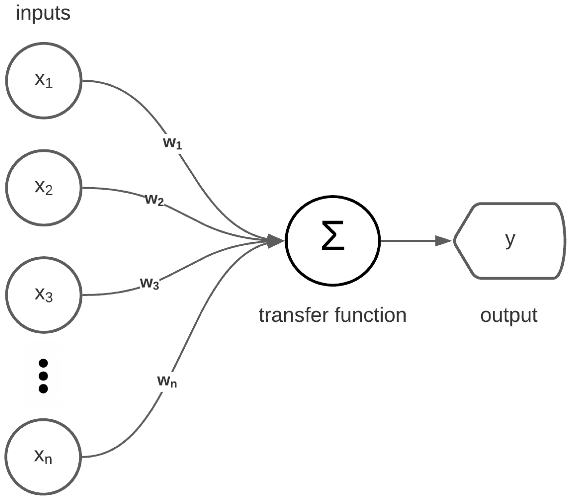
An ANN is a network of interconnected neurons that translate an input to an output using weights and transfer functions. A flowchart of a simple ANN is shown in Figure 8. Here, the inputs () are multiplied by their weights (), with the result being summed and used as input for the transfer function of the neuron. The result of the transfer function is then used as input for the output function. This output function is a linear function for regression. The output function gives the output (). The difference between the predicted value and the observed value is then used to change the weights of the ANN. This can be performed using various techniques, with the most common approach being back-propagation with stochastic gradient descent [22]. The transfer function of a neuron can be a linear function, sigmoid function, or any other function. When the ANN is expanded to use more inputs and neurons, all inputs are connected to every neuron with individual weights. One can add as many neurons, inputs. and outputs as desired and can also vary the amount of layers of neurons. The parameters not trained by the neural network, such as the choice of the number of neurons and the type of transfer functions, are called hyper-parameters.
A recurrent neural network is a type of artificial neural network (ANN) that uses the output of previous time steps () as input for the current time step (). Therefore, the RNN is better equipped to predict time series than traditional ANNs [23]. However [24] have shown that a simple RNN can barely store information for longer than 10 time steps. Therefore, other approaches to an RNN have been studied, with one of the most commonly applied being the LSTM proposed by [20]. More specifically, [15] compared the accuracy of various neural network approaches in predicting sewer overflows. Even though the LSTM had a relatively slower learning curve, the results of this type of neural network were most promising for multi-step-ahead predictions [15]. This is because an LSTM has an added cell state that is updated using transfer functions at each time step. This cell state is also used to predict the output of each time step, making it possible to store information for a longer period.
4.2. The LSTM Set-Up
The sewer model input is a spatially uniform precipitation intensity time series, and the output is a flood volume for each time step at each manhole in the studied area. The LSTM is a ‘one-to-one’ recurrent neural network. This means that for each timestep of the input, an output is calculated. The timesteps for the precipitation input time series, sewer model output, and LSTM predictions are thus all equal to 5 min. Furthermore, the LSTM set-up is similar to that of the sewer model with 1 input, 1 hidden layer, and 230 outputs (1 for each manhole). The number of neurons in the hidden layer and the learning rate are determined using hyper-parameter optimisation. The LSTM is constructed using Keras [25]. Keras is a high-level library used for machine learning applications. Keras runs on Tensorflow [26], which is an open source machine learning software released by Google in 2015.
The synthetic input–output data set, created with the sewer model, is split into training, testing, and validation data sets. The training data are used to find an optimal set of connection weights, the test data are used to choose the best network configuration (i.e., the hyperparameters: in this study, the number of neurons and the learning rate), and the validation set is only used to evaluate the LSTM’s final performance in terms of generalization ability [27].
The data set is divided according to the average of studies studied by [16]. They found that , , and of the total data were used for training, testing, and validation, respectively. In the present study, a split of , , and is used. The input precipitation time series are normalised to a range.
For the determination of the hyper-parameters of the LSTM, Bayesian hyper-parameter optimisation is used. Due to the long training times for each configuration of the LSTM (60 min+), grid search or random search hyper-parameter optimisation was not feasible. The hyper-parameters determined were the number of neurons of the LSTM layer and the learning rate. The sequential model built with Keras is comprised of two layers. The first layer is the LSTM layer, in which the transfer functions were set to the standard functions. The second layer is a Dense layer. This layer is a standard ANN layer of neurons with a linear activation function. The layer consists of 230 units, which coincides with the amount of target outputs in the model. The sequential model is compiled using the MAE loss function for training.
4.3. The Performance Indicators
The performance indicators used to assess the predictive capability of the trained LSTM are Nash-Sutcliffe efficiency (NSE) and coefficient of determination . The MAE is used to train and test the LSTM, and the NSE and are used to assess the predictive ability of the LSTM on the validation data set.
The calculation of the MAE is shown in Equation (1). A value of 0 shows a perfect fit between the observed and predicted values:
in which is the i-th predicted value, and is the i-th observed value.
The NSE is commonly used as a predictive measure of hydrological models. For some precipitation events, manholes in the north of the area had NSE values approaching negative infinity. No flooding occurred at these manholes and the (negative) flood volumes in the sewer model results. However, the LSTM still predicted relatively high fluctuations. The scale of these fluctuations were small, causing no wrong predictions in flooding. These fluctuations around the mean did result in the NSE values approaching negative infinity. Therefore, the bounded version of the NSE, proposed by [28] and called C2M (see Equation (2)), is applied instead. NSE values are now bounded to the interval , providing a more usable mean NSE value of all manholes in the area:
in which is the mean of the predicted values, and is the mean of the observed values.
The last performance indicator used is the . The measures the correlation between the observed and predicted values. The Equation for is shown in Equation (3):
5. Results
5.1. LSTM Validation Based on Synthetic Precipitation Events
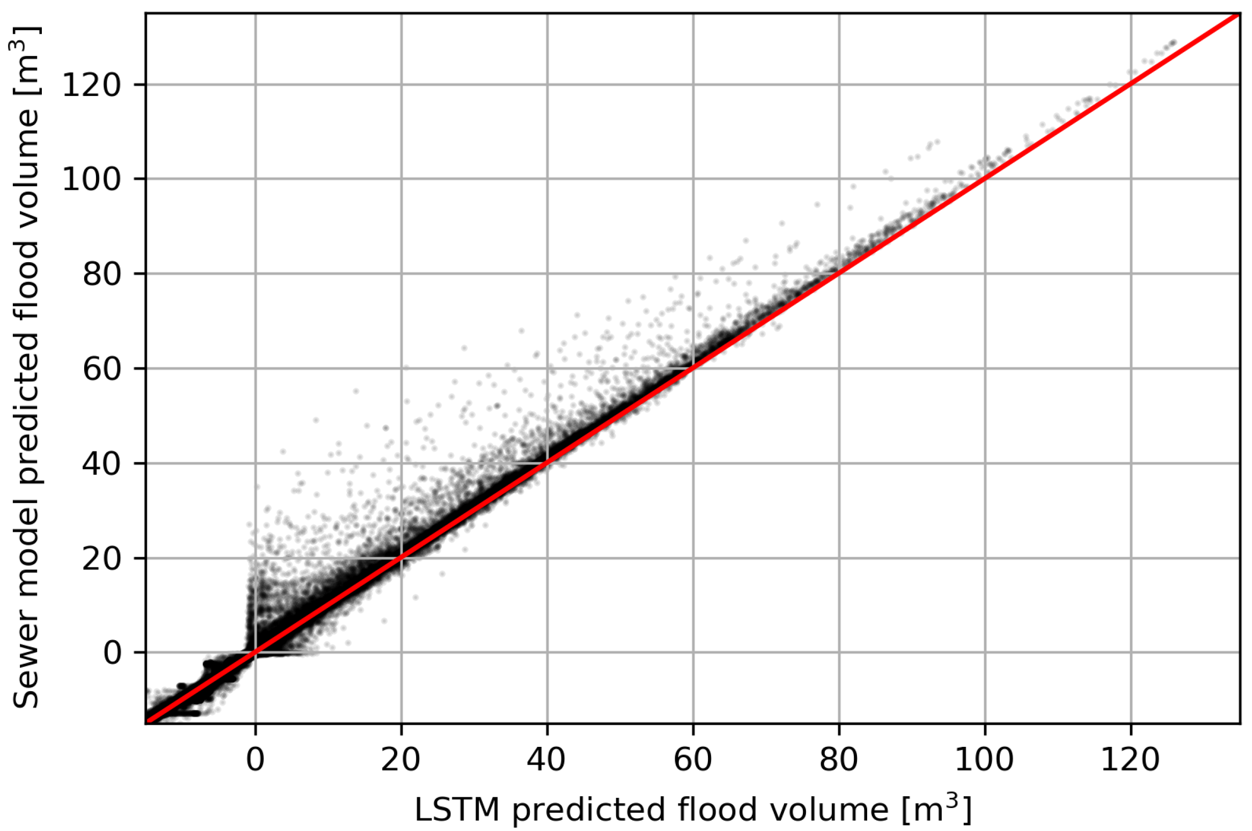
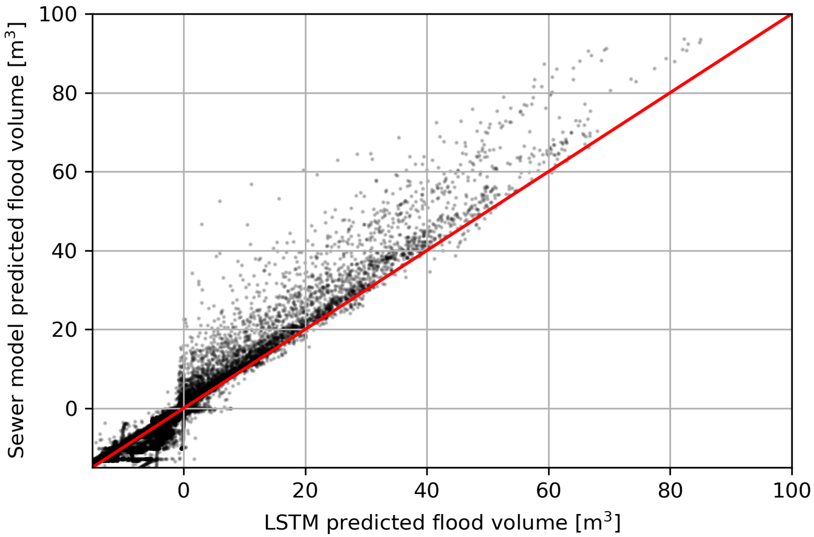
After Bayesian optimisation, the LSTM has 636 neurons to predict the flood volumes at the 230 manholes accurately and a learning rate of . The total run time of the LSTM on the 25 precipitation events present in the validation data set was 1.89 s. During this validation, the LSTM was capable of predicting if a manhole will flood with an accuracy 99.60% (with a threshold value of 1 m). Only in 0.26% of the precipitation events was a flood predicted by the LSTM, while no flooding occurred during the sewer model simulation (LSTM prediction > 1 m3 and sewer model prediction < 1 m3 in Figure 9). Only in 0.14% of the precipitation events was the opposite applied, meaning that the LSTM did not predict a flood while flooding occurred according to the sewer model (LSTM prediction < 1 m3 and sewer model prediction > 1 m3 in Figure 9). This high accuracy, in combination with the extremely low computation time, shows the potential of using an LSTM as an early flood-warning system.
Furthermore, the flood volumes were predicted with high accuracy by the trained LSTM. An average R2 of 0.99 and an average NSE of 0.87 for all manholes was found (Table 2). However, only 38% of the manholes in the studied area experienced flooding on the validation data set. The manholes that did not flood show a relatively low goodness-of-fit. In these cases, the sewer model predicted mostly an almost constant negative flood volume that varied slightly over time. A negative flood volume predicted by the sewer model means that the water level is below the surface level and thus no flooding occurs. For these situations, the LSTM predicts larger negative flood volume fluctuations since the LSTM is sensitive to any change in the input parameters: even a small change in the precipitation results in a different predicted flood volume. However, these volume fluctuations predicted by the LSTM were still below 0.1 m3 and not relevant for flood forecasting purposes.
Since the manholes that do not flood are not interested from an early flood warning perspective, we only focus on the results of the flooded manholes. Figure 9 shows the predicted flood volumes of the LSTM and sewer model for each time step of the 25 precipitation events present in the validation data. It shows that the LSTM predictions closely resemble the sewer model output since most data points follow the linear 1:1 line. However, the LSTM tends to slightly underpredict the flood volumes, and especially the peak, compared to the sewer model output. On average, the peak values are underpredicted by 8.5% by the LSTM. This behaviour is a well-known problem with neural networks since they are prone to systematically underpredict flood series for extreme events [13]. If accurate prediction of the peak values is of high importance, LSTM performance can be increased by, for example, postprocessing the flood volume predictions by applying an unscented Kalman filter [29].
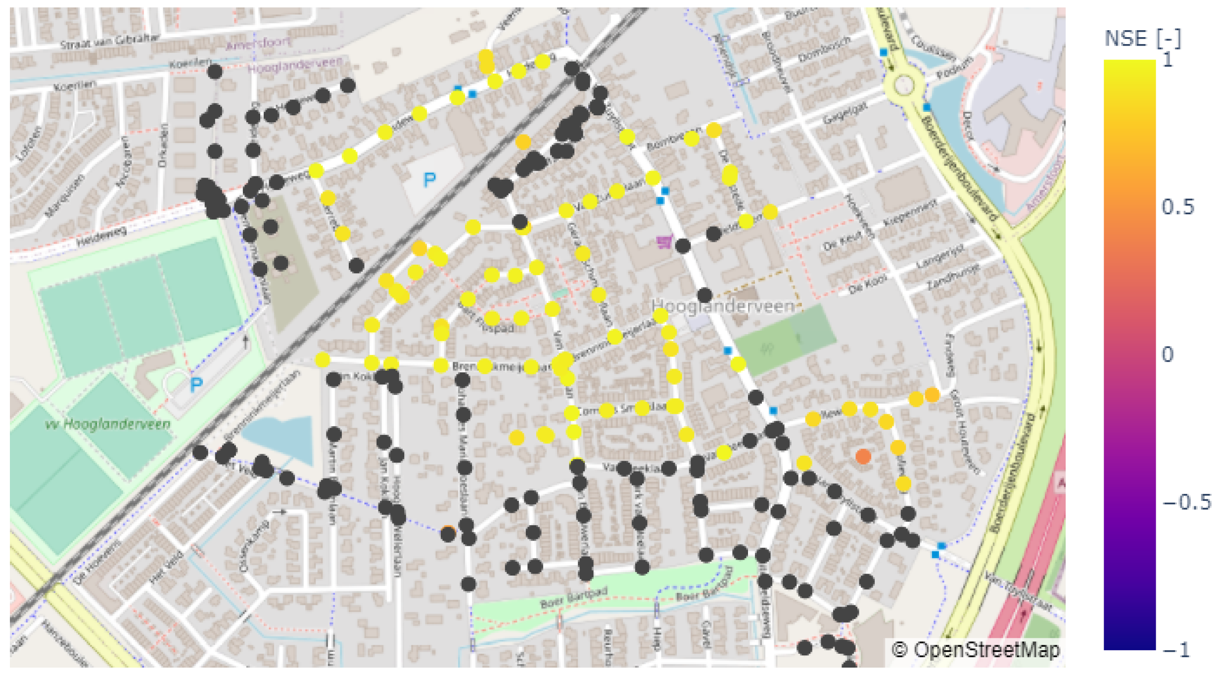
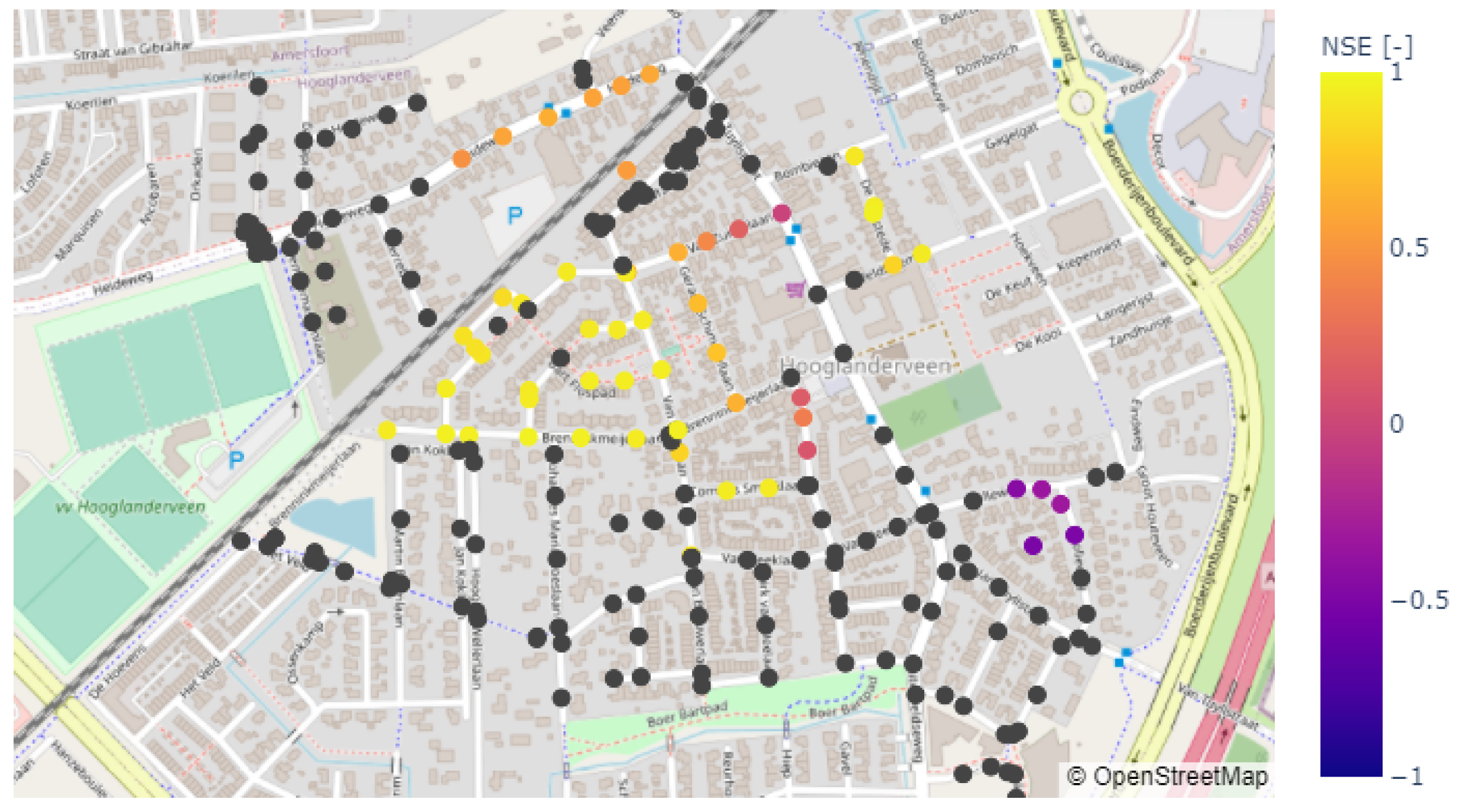
A map with the NSE values for the flooded manholes is shown in Figure 10. The NSE values vary between 0.39 and 0.99, with an average value of 0.92. Higher NSE values are generally found in the centre and northwest of the study area, where the most severe flooding occurs. The LSTM predictions were less accurate in the southeastern region of the study area, where the manholes only experience minor flooding because of the relatively high surface levels.
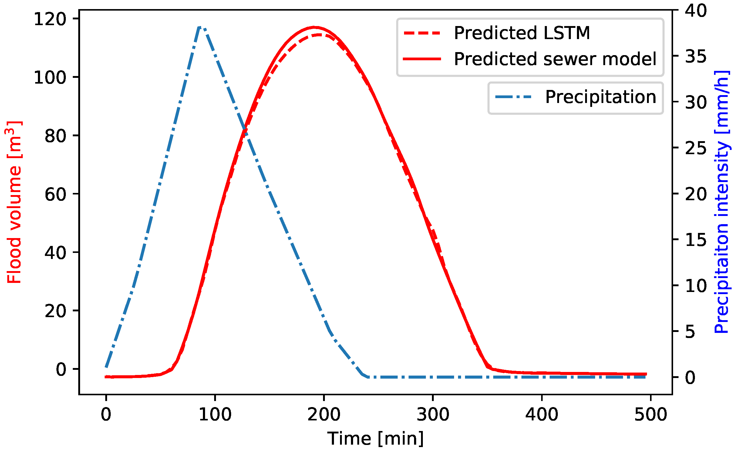
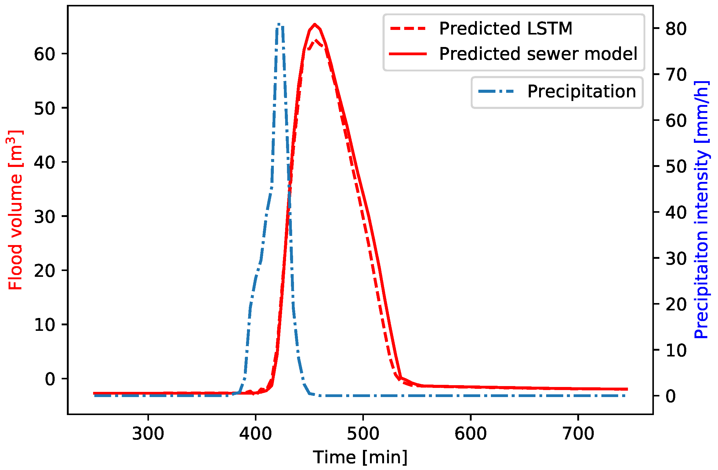
Figure 11 shows the predicted flood volumes both by the LSTM and sewer model for a manhole located in the centre of the study area, where extreme flooding occurs at most manholes. This manhole has an average NSE of 0.95. A lag is generally present between the peak of the precipitation event and the moment that flooding of the manholes starts to occur. The LSTM is able to predict this lag with high accuracy when compared to the sewer model output. Furthermore, the LSTM is capable of predicting the general shape of the flood volume hydrograph accurately, both in terms of the timing that flooding starts to occur as well as the timing of the peak flood volume. However, again, the slight tendency of the LSTM to underpredict the peak flood volumes is visible.
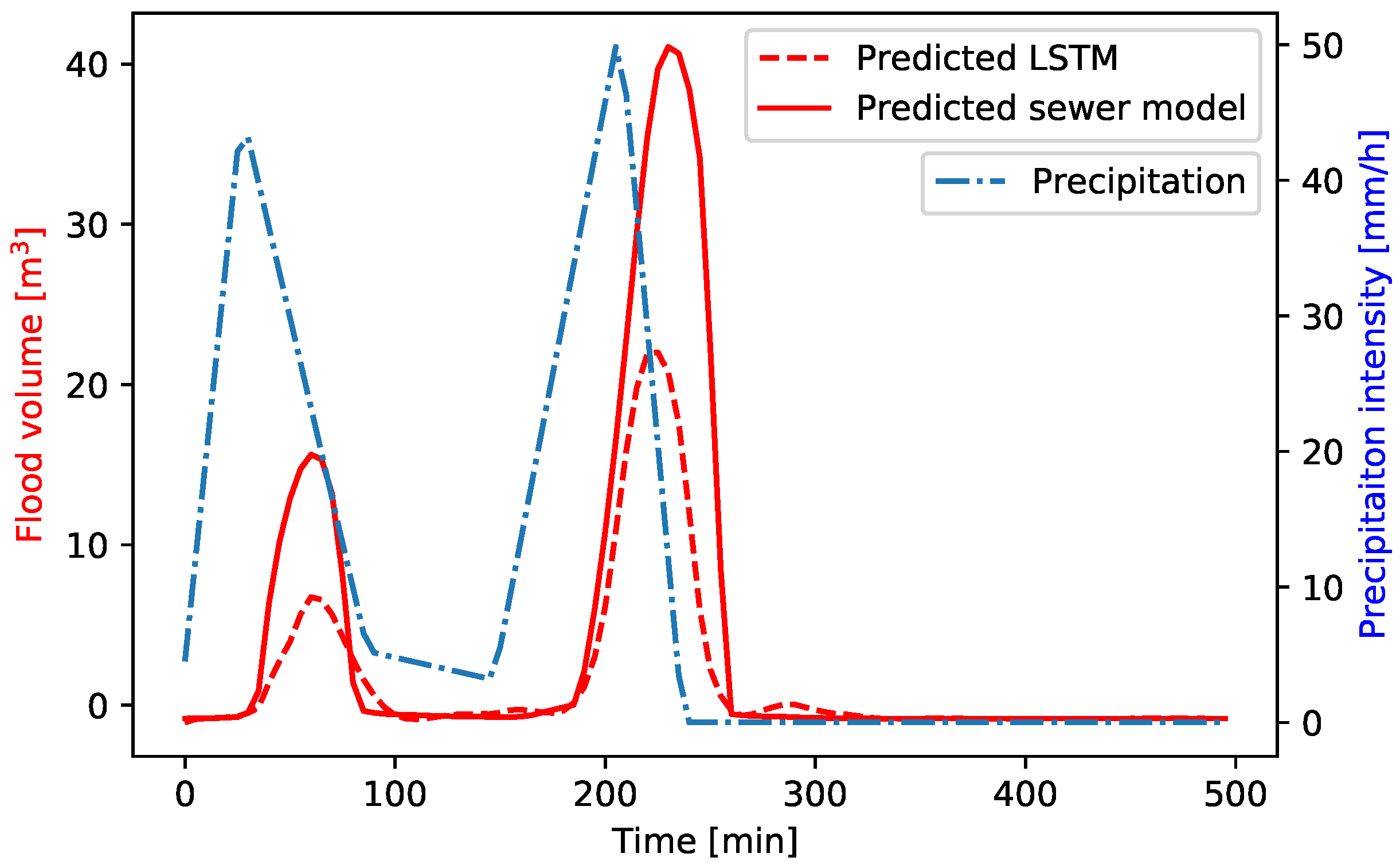
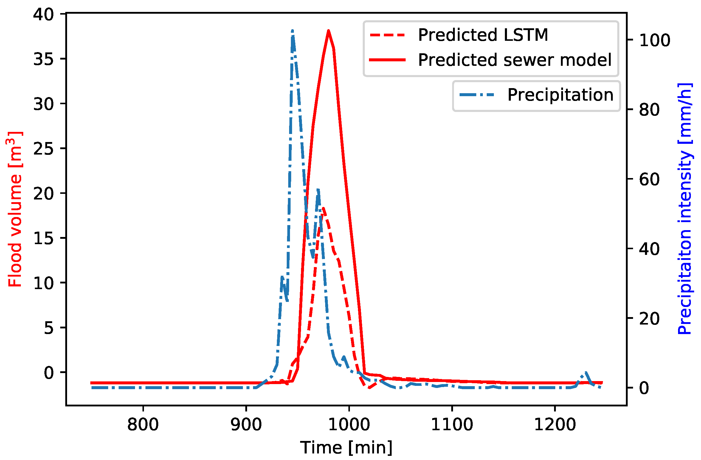
The predicted flood volumes by the sewer model and LSTM for a manhole located in the southeastern part of the study area are shown in Figure 12. Here, the LSTM has an average NSE of 0.39. Again, the shape of the flood hydrograph is predicted accurately, even when a two-peaks event is considered. However, the underprediction of the peak value is larger in this region of the study area. It seems that the LSTM has more difficulties in accurately predicting flood volumes in cases of relatively sharp flood volume hydrographs, with large differences between the flood volumes in two consecutive time steps. The accuracy of the LSTM predictions can therefore be improved by reducing the time step of the training data set such that the change in flood volume within two consecutive time steps is reduced.
5.2. LSTM Evaluation Based on Historic Precipitation Events
To further test the LSTM, three historic precipitation events that caused flooding in the area were identified. These historic precipitation events were simulated both by the sewer model and LSTM network to predict corresponding flood volumes. Again, the performance of the LSTM model is compared against the sewer model predictions since this model is used to train the LSTM. For this reason, the LSTM performance is at maximum as good as the sewer model, and comparing LSTM predictions with field measurements does not give a proper indication of the LSTM performance.
Also on the historic data set, the LSTM shows the high potential to be used as an early flood warning system. In 94.4% of the precipitation events, the LSTM predicted correctly if flooding occurred at one of the manholes (with a threshold of 1 m3). Only in 4.6% of the precipitation events was a flood predicted by the LSTM, while no flooding occurred during the sewer model simulation. Only in 1.0% of the precipitation events did the LSTM not predict a flood while flooding occurred. This shows that the number of false positive and false negative flood predictions has not increased compared to the validation using the synthetic data set. Therefore, the ability of the LSTM to predict if a flooding occurs even holds for scenarios deviating from those used during the training procedure.
Figure 13 shows the predicted flood volumes by the LSTM and sewer model for each time step of the three historic precipitation events. This figure also shows that the LSTM is able to predict if flooding occurs accurately. However, the tendency to underpredict flood volumes is again present and is even more severe compared to the validation results based on the synthetic data set. On average, the peak flood volumes are underpredicted by 34.3%.
During the validation based on the synthetic data set (Section 5.1), we found that the average NSE increases if only the manholes that experience flooding are considered. When we test the LSTM performance on historic precipitation events, we find an average NSE of 0.57 if only the flooded manholes are considered, while an average NSE of 0.61 is found for all manholes (Table 3). This is probably caused by the low LSTM performance for the manholes in the southeastern region (Figure 14), where the flood volume time series show complex behaviours.
Figure 15 and Figure 16 show the predicted flood volumes by the LSTM and sewer model for a manhole in the centre (NSE = 0.96) and southeast (NSE = −0.50) of the study area, respectively. The hydrograph shape, in terms of the timing that flooding starts to occur and the timing of the peak value, are predicted with high accuracy for the manhole located in the centre of the study area. This shows that the LSTM performance does not significantly change compared to the validation results on the synthetic data set for the region, where the most frequent and severe flooding occurs. On the other hand, the predictive ability in the southeastern region has decreased (Figure 16). Especially, the peak flood volume is underpredicted significantly. However, again, the timing that flooding starts to occur and the timing of the peak value are captured accurately by the LSTM. This shows that, despite the fact that the total flood volumes are underpredicted, the LSTM still has potential to be used as an early flood warning system in these regions.
The lower LSTM performance on the historic data set, compared to the synthetic data set, is probably caused by the fact that the historic precipitation peaks are confined in a smaller time span, compared to the synthetic training data set. Also in the synthetic training data set, we already found that the the LSTM’s performance decreases for the manholes where the flooding occurred in a relatively small time span (Figure 12). Furthermore, the lower performance of the LSTM on historic rainfall events can be explained by the small fluctuations and/or noise in the precipitation data. This shows that, in general, the LSTM performs best when large and smooth precipitation intensities are given as input, resulting in large flood volume time series and matching the precipitation patterns from the synthetic training data set.
To increase the predictive ability of the LSTM, two adjustments are proposed: First, the time step used in this study was 5 min. Due to the sudden nature of extreme precipitation events, this relatively long time step results in a large increase in the flood volumes in two consecutive time steps. Therefore, we recommend reducing this time step, which will only increase the computation time of the sewer model used to generate the training data and barely that of the LSTM. Second, the precipitation statistics were given in patterns with a time step of 1 h. In this study, this pattern was linearly interpolated. By adjusting this interpolation approach, the sharp hydrographs observed in the historic data can be recreated in the synthetic data set, ensuring that more events with confined peaks are included in the training data set.
6. Discussion
Many studies use historic data to train neural networks (e.g., [5,8,10,15]). However, in this study, input–output relations of a numerical sewer model were used to train the LSTM network. Furthermore, synthetic precipitations events were used to create the training data set, adding two additional levels of abstraction from reality (e.g., [13,30,31]). Making use of synthetic precipitation events ensures that a wide range of precipitation characteristics, in terms of precipitation pattern, intensity, and duration, can be included systematically. Section 5.2 showed that, even though the LSTM was trained on synthetic precipitation events, it still accurately predicts which manholes will flood. This indicates that the LSTM is able to respond to precipitation events not present in the training data accurately due to the wide variety of events included in the training data set. This even applies for precipitation events having higher rainfall intensities than present in the training data.
It must be noted that the developed LSTM only predicts flood volumes at maximum as accurate as the sewer model used to train the LSTM. This means that errors present in the sewer model are inherently also present in the LSTM. Additionally, the LSTM is only capable of predicting reliable outputs for the conditions it was trained for. For two historic flood events, not presented in this paper, we found that flooding was observed by inhabitants of Hooglanderveen while the sewer model, and consequently the LSTM, did not predict any flooding. During these events, the measured precipitation intensities were relatively low and would most likely not lead to any flooding in the area under normal circumstances. Therefore, it might be that the inflow of some manholes was blocked by leaves during the precipitation event, causing the inundation of the streets. The sewer model was not designed to model these rare events and hence the LSTM is also not able to include these processes in the predictions.
The computational costs of the LSTM are extremely low, with forecasting times in the order of milliseconds for a single event. Due to the inherent variability in extreme flood events, and the need for ensemble forecasting, many simulations are required. The LSTM can be applied successfully for this purpose, providing a probability of flood volumes instead of a deterministic forecast. This can be helpful for decision makers in their assessment of possible damages caused by the extreme precipitation event.
Regarding the set-up of the LSTM, it was decided to develop a single LSTM network for the entire Hooglanderveen sewer system. This has as advantage that flood volumes at all manholes are computed based on a single input precipitation event. However, setting up an LSTM network for the entire system increases the complexity of the network significantly, compared to having a separate LSTM for each manhole. Consequently, the training time is also significantly higher. Kratzert et al. [8] analysed the effect of setting up a single LSTM to predict rainfall runoff for multiple catchments compared to using multiple regional LSTMs each trained for a single catchment. They found that using a single LSTM network to predict the runoff for multiple catchments results in slightly more accurate predictions, especially in cases with a strong correlation in the predicted output at the various catchments. Furthermore, they suggest that using a single LSTM for an entire network reduces the risk of overfitting compared to setting up an LSTM network for each desired output location [8]. For these reasons, setting up a single LSTM network to predict all manholes in a sewer system is recommended despite the long training times involved.
7. Conclusions
The objective of this research was to construct an LSTM neural network that can predict location-based flooding due to extreme precipitation in an urban environment. For the first time, such an LSTM was developed for a large sewer system covering many manholes. Because insufficient measured data of extreme precipitation events were available, a numerical sewer model was used to generate the training data covering a wide variety of synthetic precipitation events in terms of precipitation intensities and patterns. The LSTM was set up for the whole area of Hooglanderveen in Amersfoort containing 230 manholes. The trained LSTM, having 636 neurons, predicted the flood volume time-series of all flooded manholes with high accuracy, resulting in an average NSE of . Furthermore, the temporal aspects of the flood wave, in terms of the duration of the flooding, as well as the timing of the peak flood volume, were accurately predicted by the LSTM. Especially the locations with frequent and severe flooding are predicted with high accuracy. Therefore, we conclude that the behaviour of the existing numerical sewer model and its characteristics were successfully reproduced by the LSTM.
Testing of the LSTM on observed historic data shows that the LSTM can also accurately predict the temporal aspects of the flooding for historic precipitation events. Using a large variety of synthetic precipitation events in the training data set ensured that the trained LSTM was able to generalise, even though the historic precipitation patterns differ from the synthetic data since the historic precipitation events are confined to a relatively short interval with high-intensity precipitation. However, it was found that the LSTM tends to underpredict flood volumes, especially for the relatively sharp flood volume hydrographs, with large differences between the flood volumes in two consecutive time steps. In this study, a relatively large time step of five minutes was used to train the LSTM. Therefore, the accuracy of the LSTM predictions can easily be improved by reducing this time step such that the change in flood volume within two consecutive time steps is reduced.
The computational costs of forecasting a single event is exceptionally low, reducing the forecasting time to the order of milliseconds, making the LSTM highly functional as an early flood warning system. Furthermore, this extremely low computational cost makes it possible to compute ensemble forecasts of pluvial flooding, using stochastic precipitation forecasts instead of a single deterministic time series.
Author Contributions
Conceptualization, R.A.H.K., A.B. and K.M.W.; methodology, R.A.H.K. and A.B.; software, R.A.H.K.; validation, R.A.H.K.; data curation, R.A.H.K.; writing—original draft preparation, R.A.H.K. and A.B.; writing—review and editing, R.A.H.K. and A.B.; visualization, R.A.H.K.; supervision, A.B. and K.M.W. All authors have read and agreed to the published version of the manuscript.
Funding
This project has received funding from the European Union’s Horizon 2020 Research and Innovation Programme under grant agreement no. 820751.
Institutional Review Board Statement
Not applicable.
Informed Consent Statement
Not applicable.
Data Availability Statement
Restrictions apply to the availability of the input data. The results of the synthetic validation data can be viewed on the following website: https://hooglanderveen-riolering-opti.herokuapp.com/, accessed on 5 May 2022. The results of the historic data test can be viewed on the following website: https://hooglanderveen-riolering-hist.herokuapp.com/, accessed on 5 May 2022.
Acknowledgments
The authors would like to thank Hydrologic for their guidance and expert advice during the research. The authors would also like to thank the Municipality of Amersfoort for providing the data related to the observed historical precipitation events. Furthermore, the authors would like to thank Arcadis for providing the input–output data of the sewer model used to train the LSTM network in this study.
Conflicts of Interest
The author declares no conflict of interest.
Abbreviations
The following abbreviations are used in this manuscript:
| MDPI | Multidisciplinary Digital Publishing Institute |
| DOAJ | Directory of Open Access Journals |
| LSTM | Long term-short term neural network |
| ML | Machine learning |
| ANN | Artificial neural networks |
| RRN | Recurrent neural networks |
References
- Szöllösi-Nagy, A.; Zevenbergen, C. Urban Flood Management; CRC Press: Boca Raton, FL, USA, 2004. [Google Scholar]
- May, W. Potential future changes in the characteristics of daily precipitation in Europe simulated by the HIRHAM regional climate model. Clim. Dyn. 2008, 30, 581–603. [Google Scholar] [CrossRef]
- Min, S.K.; Zhang, X.; Zwiers, F.W.; Hegerl, G.C. Human contribution to more-intense precipitation extremes. Nature 2011, 470, 378–381. [Google Scholar] [CrossRef] [PubMed]
- Ayazpour, Z.; Bakhshipour, A.E.; Dittmer, U. Combined Sewer Flow Prediction Using Hybrid Wavelet Artificial Neural Network Model. In Proceedings of the New Trends in Urban Drainage Modelling; Mannina, G., Ed.; Springer International Publishing: Cham, Switzerland, 2019; pp. 693–698. [Google Scholar]
- Mounce, S.R.; Shepherd, W.; Sailor, G.; Shucksmith, J.; Saul, A.J. Predicting combined sewer overflows chamber depth using artificial neural networks with rainfall radar data. Water Sci. Technol. 2014, 69, 1326–1333. [Google Scholar] [CrossRef]
- Razavi, S.; Tolson, B.A.; Burn, D.H. Review of surrogate modeling in water resources. Water Resour. Res. 2012, 48, 1–32. [Google Scholar] [CrossRef]
- Sit, M.; Demiray, B.Z.; Xiang, Z.; Ewing, G.J.; Sermet, Y.; Demir, I. A comprehensive review of deep learning applications in hydrology and water resources. Water Sci Technol. 2020, 82, 2635–2670. [Google Scholar] [CrossRef] [PubMed]
- Kratzert, F.; Klotz, D.; Brenner, C.; Schulz, K.; Herrnegger, M. Rainfall–runoff modelling using Long Short-Term Memory (LSTM) networks. Hydrol. Earth Syst. Sci. 2018, 22, 6005–6022. [Google Scholar] [CrossRef] [Green Version]
- Bomers, A.; van der Meulen, B.; Schielen, R.M.J.; Hulscher, S.J.M.H. Historic flood reconstruction with the use of an Artificial Neural Network. Water Resour. Res. 2019, 55, 9673–9688. [Google Scholar] [CrossRef] [Green Version]
- Liu, P.; Wang, J.; Sangaiah, A.K.; Xie, Y.; Yin, X. Analysis and Prediction of Water Quality Using LSTM Deep Neural Networks in IoT Environment. Sustainability 2019, 11, 2058. [Google Scholar] [CrossRef] [Green Version]
- Poornima, S.; Pushpalatha, M. Prediction of Rainfall Using Intensified LSTM Based Recurrent Neural Network with Weighted Linear Units. Atmosphere 2019, 10, 668. [Google Scholar] [CrossRef] [Green Version]
- Zou, R.; Lung, W.S.; Wu, J. An adaptive neural network embedded genetic algorithm approach for inverse water quality modeling. Water Resour. Res. 2007, 43, 8. [Google Scholar] [CrossRef] [Green Version]
- Bomers, A. Predicting Outflow Hydrographs of Potential Dike Breaches in a Bifurcating River System Using NARX Neural Networks. Hydrology 2021, 8, 87. [Google Scholar] [CrossRef]
- Rjeily, Y.A.; Abbas, O.; Sadek, M.; Shahrour, I.; Chehader, F.H. Flood forecasting within urban drainage systems using NARX neural network. Water Sci. Technol. 2017, 76, 2401–2412. [Google Scholar] [CrossRef] [PubMed]
- Zhang, D.; Lindholm, G.; Ratnaweera, H. Use long short-term memory to enhance Internet of Things for combined sewer overflow monitoring. J. Hydrol. 2018, 556, 409–418. [Google Scholar] [CrossRef]
- Rajaee, T.; Ebrahimi, H.; Nourani, V. A review of the artificial intelligence methods in groundwater level modeling. J. Hydrol. 2019, 572, 336–351. [Google Scholar] [CrossRef]
- Rioned, S. Kennisbank. Available online: https://www.riool.net/kennisbank (accessed on 27 November 2020).
- Henonin, J.; Russo, B.; Mark, O.; Gourbesville, P. Real-time urban flood forecasting and modelling—A state of the art. J. Hydroinform. 2013, 15, 717–736. [Google Scholar] [CrossRef]
- Beersma, J.; Hakvoort, H.; Jilderda, R.; Overeem, A.; Versteeg, R. Neerslagstatistiek en Reeksen Voor Het Waterbeheer; Stichting Toegepast Onderzoek Waterbeheer: Amersfoort, The Netherlands, 2019. [Google Scholar]
- Hochreiter, S.; Schmidhuber, J. Long Short-Term Memory. Neural Comput. 1997, 9, 1735–1780. [Google Scholar] [CrossRef]
- Yu, Y.; Si, X.; Hu, C.; Zhang, J. A Review of Recurrent Neural Networks: LSTM Cells and Network Architectures. Neural Comput. 2019, 31, 1235–1270. [Google Scholar] [CrossRef]
- Goodfellow, I.; Bengio, Y.; Courville, A.; Bengio, Y. Deep Learning; MIT Press: Cambridge, MA, USA, 2016; Volume 1. [Google Scholar]
- Elman, J.L. Finding Structure in Time. Cogn. Sci. 1990, 14, 179–211. [Google Scholar] [CrossRef]
- Bengio, Y.; Simard, P.; Frasconi, P. Learning long-term dependencies with gradient descent is difficult. IEEE Trans. Neural Netw. 1994, 5, 157–166. [Google Scholar] [CrossRef]
- Chollet, F. Keras. 2015. Available online: https://github.com/fchollet/keras (accessed on 15 November 2020).
- Abadi, M.; Agarwal, A.; Barham, P.; Brevdo, E.; Chen, Z.; Citro, C.; Corrado, G.S.; Davis, A.; Dean, J.; Devin, M.; et al. TensorFlow: Large-Scale Machine Learning on Heterogeneous Systems. 2015. Available online: tensorflow.org (accessed on 15 November 2020).
- Bowden, G.J.; Maier, H.R.; Dandy, G.C. Optimal division of data for neural network models in water resources applications. Water Resour. Res. 2002, 38, 2-1–2-11. [Google Scholar] [CrossRef] [Green Version]
- Mathevet, T.; Michel, C.; Andréassian, V.; Perrin, C. A bounded version of the Nash-Sutcliffe criterion for better model assessment on large sets of basins. IAHS Publ. 2006, 307, 211–219. [Google Scholar]
- Zhou, Y.; Guo, S.; Xu, C.Y.; Chang, F.J.; Yin, J. Improving the Reliability of Probabilistic Multi-Step-Ahead Flood Forecasting by Fusing Unscented Kalman Filter with Recurrent Neural Network. Water 2020, 12, 578. [Google Scholar] [CrossRef] [Green Version]
- Kabir, S.; Patidar, S.; Xia, X.; Liang, Q.; Neal, J.; Pender, G. A deep convolutional neural network model for rapid prediction of fluvial flood inundation. J. Hydrol. 2020, 590, 125481. [Google Scholar] [CrossRef]
- Lin, Q.; Leandro, J.; Wu, W.; Bhola, P.; Disse, M. Prediction of Maximum Flood Inundation Extents With Resilient Backpropagation Neural Network: Case Study of Kulmbach. Front. Earth Sci. 2020, 8, 332. [Google Scholar] [CrossRef]
Figure 1.
Flow chart of the steps taken in the present research to set up an LSTM that is able to predict inundation volumes at manhole locations.
Figure 1.
Flow chart of the steps taken in the present research to set up an LSTM that is able to predict inundation volumes at manhole locations.

Figure 2.
Location of the study area of Hooglanderveen in Amersfoort, The Netherlands.

Figure 3.
Locations of important structures in the studied area and the level of sewer piping.

Figure 4.
Precipitation intensity curves, the dashed black lines indicate maximum and minimum for the 4, 8, and 12 h durations.
Figure 4.
Precipitation intensity curves, the dashed black lines indicate maximum and minimum for the 4, 8, and 12 h durations.

Figure 5.
Seven precipitation patterns for a duration of 8 h, with (a) Uniform; (b) 1 peak—12.5%; (c) 1 peak—37.5%; (d) 1 peak—62.5%; (e) 1 peak—87.5%; (f) 2 peaks—short; and (g) 2 peaks—long.
Figure 5.
Seven precipitation patterns for a duration of 8 h, with (a) Uniform; (b) 1 peak—12.5%; (c) 1 peak—37.5%; (d) 1 peak—62.5%; (e) 1 peak—87.5%; (f) 2 peaks—short; and (g) 2 peaks—long.

Figure 6.
Example interpolation of an eight hour precipitation pattern with a peak of of the total precipitation (precipitation pattern as given in Figure 5c).
Figure 6.
Example interpolation of an eight hour precipitation pattern with a peak of of the total precipitation (precipitation pattern as given in Figure 5c).

Figure 7.
Precipitation time series for historic flood events in Hooglanderveen. All time series start one day prior to the reported flooding, as there can be a delay in reporting. This can be seen with precipitation events 1 and 2.
Figure 7.
Precipitation time series for historic flood events in Hooglanderveen. All time series start one day prior to the reported flooding, as there can be a delay in reporting. This can be seen with precipitation events 1 and 2.

Figure 8.
An illustration of a simple ANN. Here, we have multiple inputs (), connected to the neuron with weights (). This output of the neuron is passed to the output () via a linear function.
Figure 8.
An illustration of a simple ANN. Here, we have multiple inputs (), connected to the neuron with weights (). This output of the neuron is passed to the output () via a linear function.

Figure 9.
Scatter plot of the predicted and actual flood volumes for the LSTM regressor evaluated on the synthetic validation data set (). Negative flood volume are plotted until −15 m3, no more false negative or false positive values are observed past this value.
Figure 9.
Scatter plot of the predicted and actual flood volumes for the LSTM regressor evaluated on the synthetic validation data set (). Negative flood volume are plotted until −15 m3, no more false negative or false positive values are observed past this value.

Figure 10.
The NSE values for each manhole in the case study area that experienced flooding from the validation data set (NSE = ). The NSE values were calculated with the predicted flood volume time series by the LSTM network and sewer model. The NSE is calculated for each time series and a mean is taken for each manhole. Dark grey manholes indicate locations where no flooding occurs.

Figure 11.
Flood volume time series, for the LSTM network validated on synthetic data, at a manhole in the centre of the area (NSE ).
Figure 11.
Flood volume time series, for the LSTM network validated on synthetic data, at a manhole in the centre of the area (NSE ).

Figure 12.
Flood volume time series, for the LSTM network validated on synthetic data, at a manhole in the southeast of the area (NSE ).
Figure 12.
Flood volume time series, for the LSTM network validated on synthetic data, at a manhole in the southeast of the area (NSE ).

Figure 13.
Scatter plot of the predicted and actual flood volumes for the LSTM regressor evaluated on the historic precipitation data set (). Negative flood volume are plotted until −15 m3, no more false negative or false positive values are observed past this value.
Figure 13.
Scatter plot of the predicted and actual flood volumes for the LSTM regressor evaluated on the historic precipitation data set (). Negative flood volume are plotted until −15 m3, no more false negative or false positive values are observed past this value.

Figure 14.
NSE values for each manhole in the case study area that experiences flooding from the historic data set (mean NSE ). NSE values have been calculated with the predicted flood volume time series by the LSTM network and sewer model. The NSE is calculated for each time series, and a mean is taken for the manholes. Dark grey manholes indicate locations where no flooding occurs.

Figure 15.
Flood volume time series, for the LSTM network validated on historic data, at a manhole in the centre of the area (NSE ).
Figure 15.
Flood volume time series, for the LSTM network validated on historic data, at a manhole in the centre of the area (NSE ).

Figure 16.
Flood volume time series, for the LSTM network validated on historic data, at a manhole in the southeast of the area (NSE ).
Figure 16.
Flood volume time series, for the LSTM network validated on historic data, at a manhole in the southeast of the area (NSE ).


Table 1.
All possible values for each precipitation event feature.
| 30 mm | Uniform | 4 h |
| 40 mm | 1 peak—12.5% | 8 h |
| 60 mm | 1 peak—37.5% | 12 h |
| 75 mm | 1 peak—62.5% | |
| 90 mm | 1 peak—87.5% | |
| 105 mm | 2 peaks—short | |
| 2 peaks—long |
Table 2.
The hyper-parameter and evaluation values of the LSTM sequential model after Bayesian optimisation.
Table 2.
The hyper-parameter and evaluation values of the LSTM sequential model after Bayesian optimisation.
| Performance Indicator | Value |
|---|---|
| NSE (all manholes) | 0.87 |
| NSE (flooding manholes) | 0.92 |
| 0.99 |
Table 3.
Performance evaluation for the LSTM tested on historic data.
| Performance Indicator | Value |
|---|---|
| NSE (all manholes) | 0.61 |
| NSE (flooding manholes) | 0.57 |
| 0.99 |
Publisher’s Note: MDPI stays neutral with regard to jurisdictional claims in published maps and institutional affiliations. |
© 2022 by the authors. Licensee MDPI, Basel, Switzerland. This article is an open access article distributed under the terms and conditions of the Creative Commons Attribution (CC BY) license (https://creativecommons.org/licenses/by/4.0/).
Share and Cite
MDPI and ACS Style
Kilsdonk, R.A.H.; Bomers, A.; Wijnberg, K.M. Predicting Urban Flooding Due to Extreme Precipitation Using a Long Short-Term Memory Neural Network. Hydrology 2022, 9, 105. https://0-doi-org.brum.beds.ac.uk/10.3390/hydrology9060105
AMA Style
Kilsdonk RAH, Bomers A, Wijnberg KM. Predicting Urban Flooding Due to Extreme Precipitation Using a Long Short-Term Memory Neural Network. Hydrology. 2022; 9(6):105. https://0-doi-org.brum.beds.ac.uk/10.3390/hydrology9060105
Chicago/Turabian StyleKilsdonk, Raphaël A. H., Anouk Bomers, and Kathelijne M. Wijnberg. 2022. "Predicting Urban Flooding Due to Extreme Precipitation Using a Long Short-Term Memory Neural Network" Hydrology 9, no. 6: 105. https://0-doi-org.brum.beds.ac.uk/10.3390/hydrology9060105
Note that from the first issue of 2016, this journal uses article numbers instead of page numbers. See further details here.