Article

Is Greenhouse Rainwater Harvesting Enough to Satisfy the Water Demand of Indoor Crops? Application to the Bolivian Altiplano

by
Juan-Manuel Sayol
1,*,
Veriozka Azeñas
2,3,
Carlos E. Quezada
3,
Isabel Vigo
1 and
Jean-Paul Benavides López
3
1
Department of Applied Mathematics, University of Alicante, Carr. de San Vicente del Raspeig, s/n, San Vicente del Raspeig, 03690 Alicante, Spain
2
Department of Biology, Universitat de les Illes Balears, Carr. de Valldemossa, km 7.5, 07122 Palma, Spain
3
Instituto de Investigaciones Socioeconómicas, IISEC-Universidad Católica Boliviana San Pablo, Av. 14 de Septiembre N° 4836, La Paz 3278, Bolivia
*
Author to whom correspondence should be addressed.
Submission received: 17 May 2022 / Revised: 8 June 2022 / Accepted: 13 June 2022 / Published: 15 June 2022

Abstract

:
As many other regions worldwide, the Bolivian Altiplano has to cope with water scarcity during dry periods, which in turn impacts on crop production as flood irrigation is overwhelmingly extended in the region. Since farming is the main income in the Altiplano for most families, the availability of greenhouses with water harvesting systems may represent a solution to warrant all year round production and food access. We study the daily satisfied water demand from a balance between rainfall collected by a greenhouse roof and water used for indoor crop irrigation assuming a tank is available for water storage. This balance is analyzed for 25 greenhouses spread over Batallas Municipality, close to Titicaca Lake, Bolivia, and for two case studies: (i) using irrigation data collected from farmers in the frame of a regional project; (ii) using theoretical daily water requirements assuming an intense greenhouse farming. Our evaluation includes a sensitivity analysis of relevant parameters, such as the influence of the time window of rainfall used in the simulation, the runoff coefficient, the roof surface area, the irrigation drip system, the irrigation frequency, the crop coefficient, the volume of water used for crop irrigation, and the capacity of the water tank. Overall, we find that the runoff coefficient has little impact on the satisfied demand rate, while all other parameters can play an important role depending on the greenhouse considered. Some greenhouses are able to irrigate crops normally during the wet season, while during the dry season, greenhouses are not able to satisfy more than 50 % of the theoretical water requirements, even when large tanks are considered. Based on these results, we recommend the construction of greenhouses with a ground surface of <50 m 2 attached to the largest available covered water tank. The information here provided can be used by stakeholders to decide their policies of investment in infrastructures in the Altiplano. Finally, the approach we follow can be applied to any other region where rainfall, temperature, and greenhouse data are available.

1. Introduction

In recent decades, global warming has exacerbated water scarcity in the Andean Altiplano. Among other impacts, we should mention the dramatic decline in the extension of tropical Andean glaciers, as described in, e.g., [1,2,3,4,5], and the rise of air temperatures [6]. It is expected that both factors will favor in the mid-term a reduction in the amount of water available for human consumption and crop irrigation [7,8,9], and will increase the water demand of crops because of the higher evapotranspiration rates [10].
The Bolivian Altiplano is characterized by long dry periods with little rainfall that can exceed six months per year, usually from April/May to September/October, which corresponds to austral autumn and winter seasons, although there are some differences between the northern and southern Altiplano in the magnitude of both rainfall and air temperatures [6,11,12]. Throughout the dry period, water is scarce and aquifers can dry up, especially during droughts episodes, thus compromising the agricultural production, and hence, the main income source of entire families. In fact, the volume of groundwater has significantly decreased in recent decades [13], which could seriously affect the amount of water available for irrigation [14]. Moreover, another factor that severely hampers the agricultural production in the Altiplano are night frosts during austral winter [15]. In addition to the strong seasonal cycle, inter-annual climate signals, such as El Niño Southern Oscillation, may boost the occurrence of droughts due to changes in the regional atmospheric flow [16,17,18].
Subsistence family agriculture encompasses almost 57% of the 130,000 farming units of the Bolivian Altiplano. This type of agriculture is greatly constrained by the low proportion of irrigated land. According to Tito and Wanderley [19], the proportion of total arable land equipped with precise irrigation during the period of 1999 and 2015 was around 7%, without any significant improvement during that period. On the other hand, the latest national agricultural survey was more optimistic and highlighted that only 26% of families dedicated to subsistence agriculture had precise irrigation. As a consequence, the remaining families use rain-fed agriculture or flood irrigation, which restricts farm production to the wet season [20]. Additionally, subsistence family agriculture does not have the financial resources to invest in technology or infrastructure to improve their income. As a result, the profit obtained from the agricultural activity is frequently insufficient for farmers in the Altiplano region [19,21,22].
Regarding the above, important investments have been made for the construction of greenhouses in Bolivia in the last three decades with mixed results [23,24,25,26]. More recently, the implementation of greenhouses with optimal use of water has been considered a key strategy within the national rural development plan for agricultural diversification, adaptation to climate change (more frequent droughts and frosts), and food security [27], with a especial focus on the Altiplano region [28,29,30]. Greenhouses help small farmers in the Altiplano to diversify their diet, improve their income, and enhance food access [26]. However, one of the limitations faced by investment in this region is the limited access to water, which is probably one of the most relevant factors for the adoption and sustained use of new agricultural technologies over time, as seen in other developing countries [31,32,33,34]. Thus, given the importance of these technologies in terms of investments, climate change adaptation, and food security policies, high-quality water usage information can help to promote sustained use of greenhouses and to increase its efficiency. On the other hand, information on the optimal water usage in greenhouses is essential from an environmental standpoint, since they can affect natural patterns and the ecological flow in the water basin, worsening the impacts of droughts [13,35].
Within the frame of a regional project, several in situ measurements were taken to get the dimensions of greenhouses (ground and roof greenhouse surface) in a rural municipality of the Bolivian Altiplano. Other information related to greenhouses infrastructure (material, installed irrigation system features) and current agricultural practices (e.g., irrigation volume, fertilization, crops cultivated, and crop rotation) were also collected. In this work, we take advantage of that information to analyze the volume of rainwater collected by greenhouse roofs in order to find the most suitable water tank capacity, according to the catalog of volumes available in the market. To this end, together with the dimension of greenhouse roofs, we consider the amount of local rainfall, the estimated irrigation frequency, the runoff coefficient, and the estimated volume of water required to satisfy the water demand of crops cultivated within greenhouses. In contrast to other works that have studied the water balance of greenhouse roofs at monthly scale, e.g., [36], we analyze the balance at daily scale, which we consider more realistic as it minimizes the water loss during intense rainfall episodes and better tracks the water caught, stored, and used in near real time. The main objective of this work is to find those greenhouses that better satisfy the water demand for agricultural purposes in greenhouses of typical rural families in the Bolivian Altiplano from two perspectives: (i) based on the irrigation procedure currently followed by local farmers, (ii) based on the water required by the most common crops if greenhouses were exhaustively cultivated.

2. Data and Methods

2.1. Greenhouse Characteristics
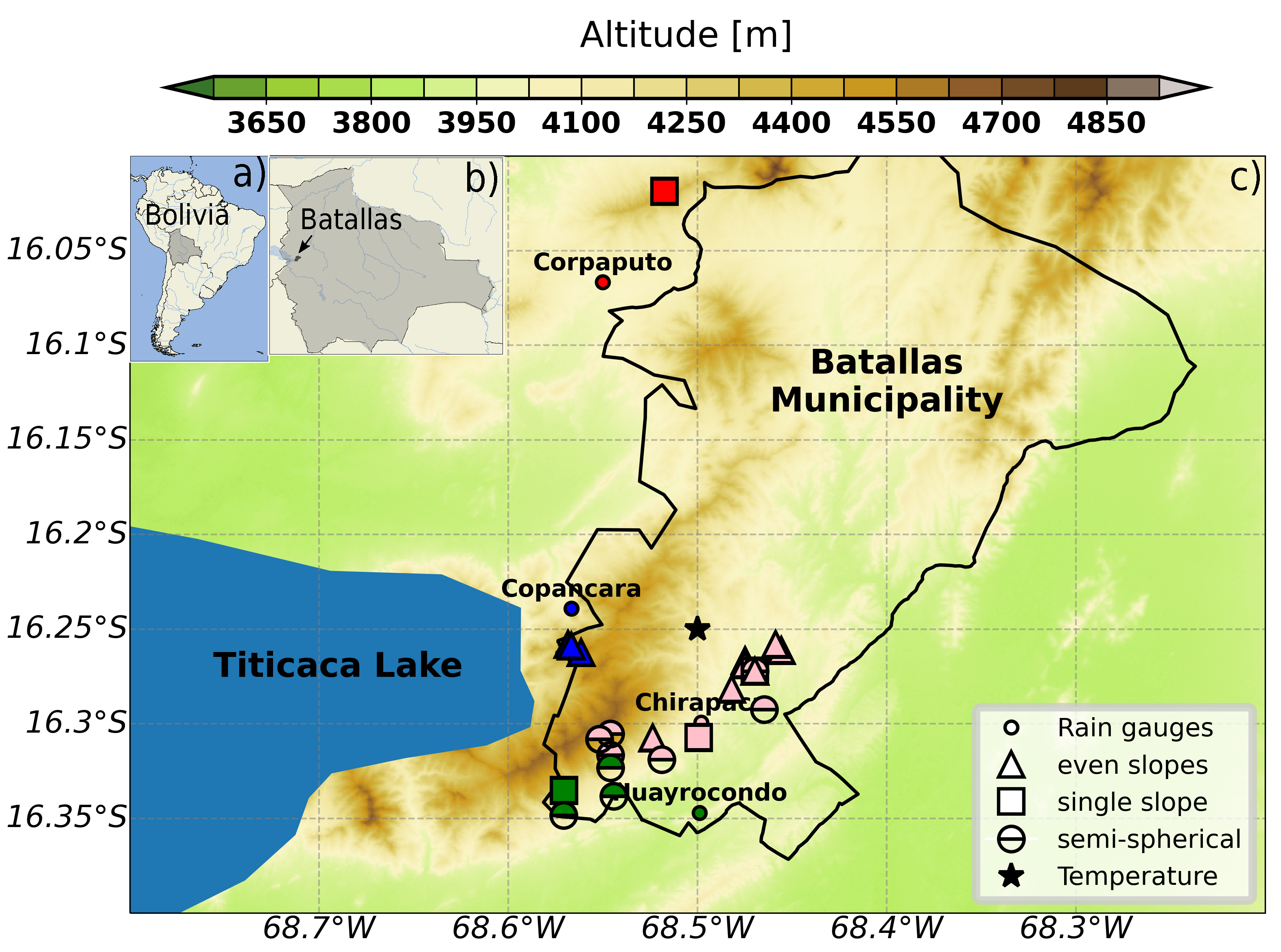
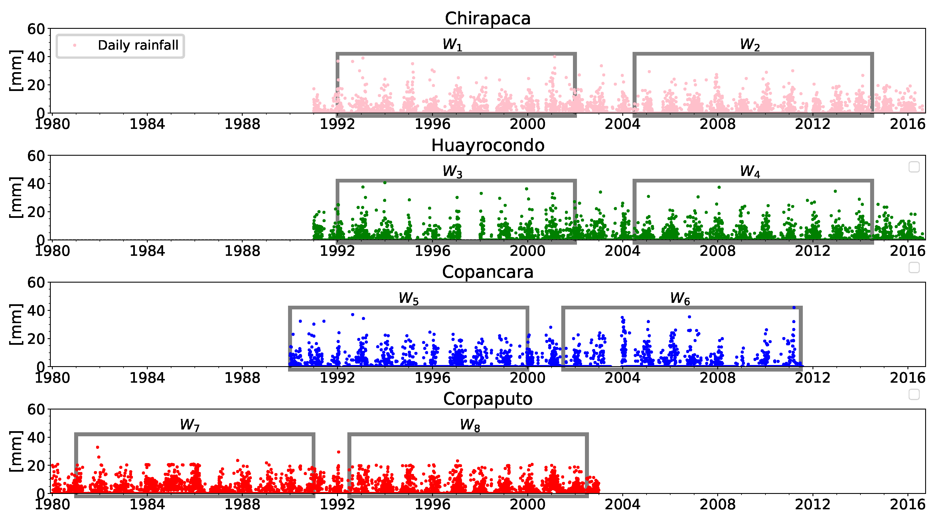
The 25 greenhouses included in the study were mostly spread across the Batallas municipality, within La Paz Department, in Bolivia, at about 4000 m height and relatively close to Titicaca Lake (Figure 1). Greenhouses were randomly selected among the close to 100 greenhouses counted in the latest available national census in the same municipality. Overall measured greenhouse roofs have three shapes, which for the selected greenhouses are illustrated in Figure 2: even or two slopes (triangles in Figure 1), Quonset or semi-spherical (semi circles in Figure 1), and single slope (squares in Figure 1). Roof measurements were performed analogically with measuring tapes (unit of cm) by experienced engineers; thus, systematic uncertainties are of the order of 0.1 m 2 using error propagation theory, which do not alter our results [37]. Table 1 summarizes greenhouse coordinates, their ground surface area, their distance to the closest rain gauge, and their catchment areas. As seen, single slope roof greenhouses are less frequent (only four), while the range of catchment areas is wide, from about 20 m 2 to around 300 m 2 .
According to the information we collected during the project, the most frequent crop is Swiss chard (Beta vulgaris subsp. vulgaris), which is being cultivated in 12 of 25 greenhouses, and the second one is lettuce (Lactuca sativa), cultivated in 8 of 25 greenhouses. Other crops, cultivated in six or fewer greenhouses, are parsley, cabbage, and celery, to mention only the most common. It is worthy to note that greenhouses usually have more than one crop, since farmers in the Altiplano tend to cultivate several species at the same time, normally between two and five, up to a maximum of seven. The main reason is that they mostly cultivate for self-consumption.

2.2. Rainfall Data

The rain gauges we use belong to SENAMHI (Servicio Nacional de Meteorología e Hidrología de Bolivia) sensors network. Those stations closest to the location of greenhouses and that cover at least two distinct time windows of 10 years of daily accumulated rainfall were selected (Figure 3). We note that the two time windows do not need to be next to each other in time, as they are used as a rough indicator to test how interannual signals such as the ENSO events affect the water demand satisfaction rate. The four selected rainfall time series have a few gaps within the time windows (<10% per month) that do not meaningfully affect the results here presented. We use a total of eight time windows ( W 1 , , W 8 , Figure 3), with time intervals and rainfall information such as the maximum daily rain, the total 10-year accumulated rain and the percentage of days with rain are shown in Table 2. The rain gauge of Corpaputo, located relatively far from all other stations, shows a slightly lower peak of daily rain (around 30 mm), but a larger total 10-year accumulated rainfall than other stations (around 2000 mm more). Indeed, on average, one in every three days, some rain is measured in Corpaputo. In contrast, the rain gauge of Copancara, closer to the Titicaca Lake, shows less accumulated 10-year rainfall and a lower percentage of rainy days (one of every six to seven days, depending on the time window, see Table 2). The largest difference in the accumulated rainfall between time windows is displayed by Chirapaca, located more inland than Copancara, with a difference of about 700 mm between W 1 and W 2 .

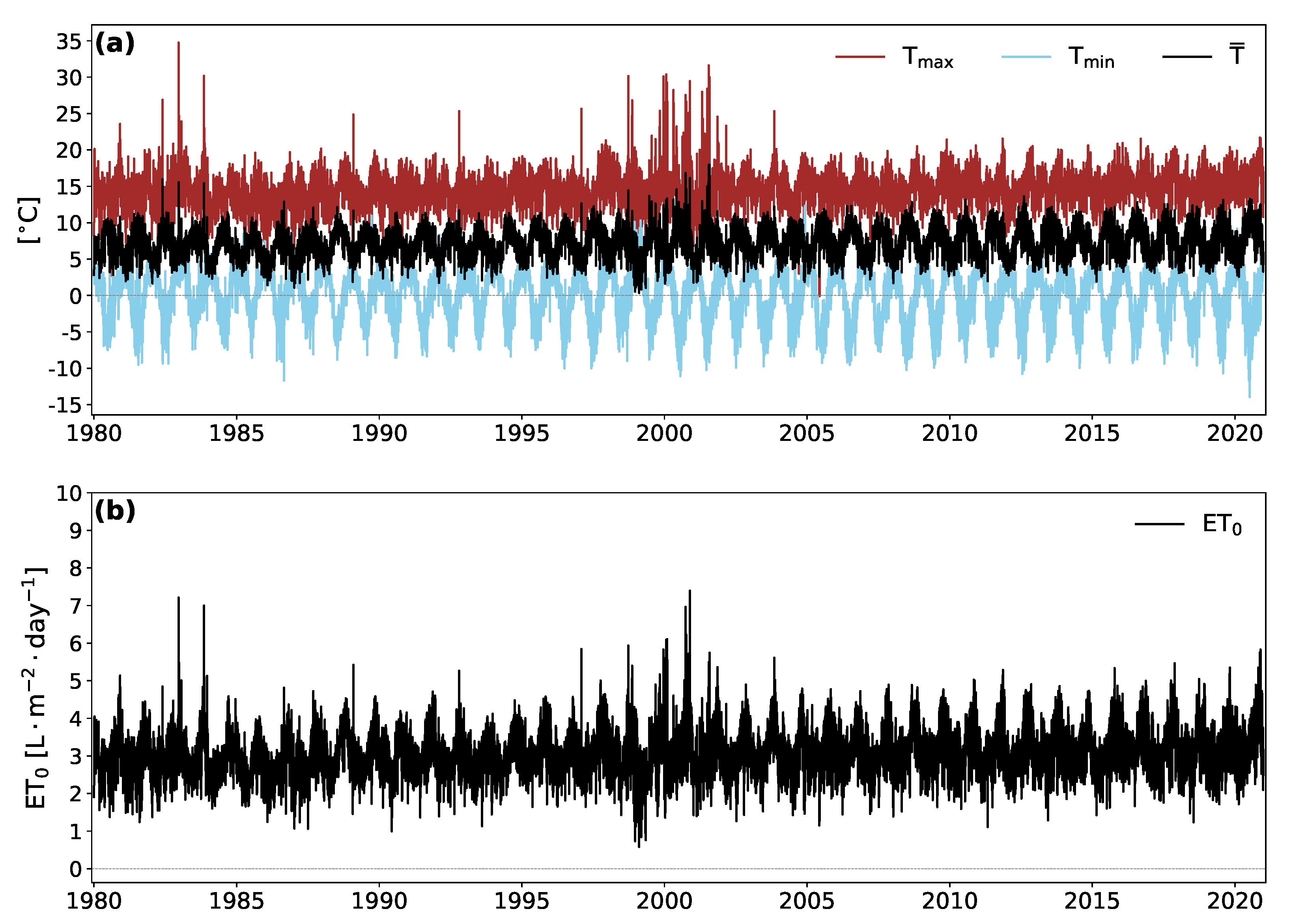
2.3. Temperature Data

In order to compute the reference evapotranspiration inside greenhouses, maximum ( T max ) and minimum ( T min ) daily air surface temperatures are required. We use CPC Global Temperature data provided by the NOAA/OAR/ESRL PSL, Boulder, CO, USA, from their website at https://psl.noaa.gov/data/gridded/data.cpc.globaltemp.html (accessed on 13 April 2022). This dataset, constructed from about 6000 to 7000 global weather stations, provides maximum and minimum daily temperatures from 1979 until the near present. It covers the whole globe and has a spatial resolution of 0.5 ° × 0.5 ° , which we consider sufficient given the smooth behavior of the temperature. Because of the relatively small surface area of Batallas Municipality, only those time series of T max and T min corresponding to the closest grid points to rain gauges are used in this analysis. In particular, we have linearly interpolated time series centered at [ 68.25 ° W, 16.25 ° S], and at [ 68.75 ° W, 16.25 ° S] in order to get time series at [ 68.5 ° W, 16.25 ° S], which falls within Batallas Municipality (depicted with a star in Figure 1). The few gaps (only 24 days over the 40 years) are filled by linear interpolation considering the closest values. Note that by construction, mean daily temperatures are easily derived as: T ¯ = T max T min 2 . Time series of maximum, mean, and minimum daily temperature are shown in Figure 4a. Time series depict a clear seasonal cycle and a range of variability between 10 ° C and 35 ° C , with average maximum and minimum temperatures of about 15 ° C and 0 ° C respectively.

2.4. Simulations of Rainwater Collected by Greenhouse Roofs

In this work, we have performed two types of simulations based on a water balance model [38,39]. These simulations incorporate the water harvested by the greenhouse roof as well as the amount of water used for irrigation. The latter is studied from both a practical and a theoretical perspective. In the first class of simulations, we depart from information provided by farmers on irrigation frequency and duration. In the second class of simulations, we hypothesize that the surface ground area of every greenhouse is cultivated with a crop (or a combination of crops) that can be characterized by an average crop coefficient. Next, we estimate the daily water irrigation requirements considering a theoretical indoor crop evapotranspiration. In particular, as reference crops, we consider Swiss chard and lettuce, by selecting crop coefficients within the range of variability reported for those crops. As mentioned above, those crops are the most common based on the information provided by farmers. Then, we simulate if harvested water is sufficient to satisfy the daily water demand considering a mean crop coefficient.
In both types of simulations, we model the daily volume of water inside a given tank volume for each greenhouse. To this end, we assume that a covered water tank is attached to the greenhouse catchment system. In this balance, we additionally hypothesize that, if any, sediments transported by first rains are collected by a filter or a small deposit before entering the water tank. For simplicity, potential loses in the gutter system are not considered here.

2.4.1. Type 1: Simulations Considering Water Irrigation Data from Farmers

The water balance equation in this case is expressed as follows:
V t t = V t t 1 + V c t C a t C h t ,
where V t t is the volume of water inside the tank at a given day and V c t the daily caught rain water, which is proportional to the vertical projection of the surface area of greenhouse roofs ( S r o o f ) over a plane, the runoff coefficient ( C r ) and the daily accumulated rainfall ( p t ): V c t = S r o o f · C r · p t [40,41].
Other terms are the daily water consumed for irrigating crops C a t , and the volume of water used for human consumption, which in this work we have fixed as C h t = 0 , t . Hence, we consider caught water is only used for agricultural purposes, although this may not be the case in reality.
As an example, if we consider a dry day, p t = 0 L, the volume of water collected will be zero, V c t = 0 L. Likewise, in those days with no irrigation, the water consumed will be identically zero, C a t = 0 L. Therefore, in any given day t, the volume inside a tank can be expressed as:
V t t = V t t 1 + V c t C a t ,
where the day we start the simulation the tank is empty, V t t 1 t = 1 = 0 . Additionally, the simulation will iterate Equation (2) during the 10-year time window selected, which is defined in Table 2 for each rain gauge. This balance also allows to track the volume of water lost when collected rainfall exceeds the capacity of a given tank, which provides an insight of which tank capacity minimizes losses. By lost water, we refer to rainfall water that can no longer be collected because the water tank is full.

2.4.2. Type 2: Simulation of Water Balance Considering Theoretical Irrigation Crop Requirements

The balance equation in this case is expressed as follows:
V t t = V t t 1 + V c t E g t · S g ,
where, again, V t t is the volume of water inside the tank at a given day and V c t is the daily harvested rain water. The new term E g t represents the crop evapotranspiration inside the greenhouse, which will depend on the growth stage and the crop considered, while S g is the cultivated surface of a given greenhouse (shown in Table 1), which is estimated as described in the following section.

2.5. Computation of Indoor Crop Water Requirements

Regarding Type 2 simulations, the approach followed to estimate crop water needs inside a greenhouse requires the computation of: (i) the outdoor reference crop evapotranspiration and (ii) the evapotranspiration of the crop of interest inside the greenhouse.

2.5.1. Reference Crop Outdoor Evapotranspiration

A widely used approach to calculate the reference crop outdoor evapotranspiration, E T 0 , is the FAO-56 Penman-Monteith equation, which is defined by local meteorological conditions (wind speed, humidity, temperature, and solar irradiation) under the assumption of a land covered by a crop of 0.12 m height, with an albedo of 0.23 and a surface resistance of 70 m s 1 . However, in Bolivia there are no available consistent measurements of humidity, and for indoor greenhouse conditions, the effect of the wind is irrelevant; for that reason, we use the simplified expression of Hargreaves and Samani [42], which has been successfully applied by Vicente-Serrano et al. [43] in Bolivia and is only fed by the extraterrestrial solar radiation, and daily maximum and minimum temperatures. It is defined as:
E T 0 = 0.0023 R a Δ T 0.5 ( T + 17.8 ) ,
which has units of L · m 2 · day 1 . T is the mean daily air surface temperature (unit of °C), Δ T = T m a x T m i n is the difference between maximum and minimum daily air surface temperatures, and R a refers to the extraterrestrial solar radiation.
To compute daily extraterrestrial radiation we use the expression:
R a = 24 ( 60 ) π I s c d r w s sin ( ϕ ) sin ( δ ) + cos ( ϕ ) cos ( δ ) sin ( w s ) ,
where I s c = 0.082 MJ · m 2 · min 1 is the solar constant, and:
d r = 1 + 0.033 cos ( 2 π 365 n )
δ = 0.4093 sin ( 2 π 365 n 1.394 )
w s = arccos tan ( ϕ ) tan ( δ )
are the distance between the Sun and the Earth, the Earth declination, and the sunset hour angle, respectively, which change for each day and with latitude. In the above expressions, n is the ordered calendar day (e.g., n = 1 corresponds to 1 January) and ϕ is the latitude (expressed in radians).
Finally, note that to get R a with the proper units ( mm · day 1 or equivalently, L · m 2 · day 1 ) we have converted it from International System units multiplying by the conversion factor ( 1 2.45 ) :
R a [ L · m 2 · day 1 ] = R a [ MJ · m 2 · day 1 ] 2.45

2.5.2. Crop Indoor Evapotranspiration

Once we obtained the reference crop evapotranspiration (Figure 4b), we estimated the evapotranspiration of a certain crop as:
E c = k c · E 0 ,
where k c is the crop coefficient specific for each species, which may change with the growth, pruning, and harvesting phases [44].
Due to the absence of wind, evapotranspiration inside the greenhouse will be smaller than outdoors. Consequently, crop evapotranspiration inside the greenhouse, E g , must be multiplied by a factor, also known as the pan coefficient, K g ( 0 , 1 ) , which depends on the local climate; hence, E g = k g · E c . As a reference, for plastic greenhouses, a factor of K g = 0.65 has been reported for Lebanon [45] and K g = 0.79 for Mediterranean conditions [46]. In our simulation, we take a factor of 0.75, since the Altiplano is less humid than the Mediterranean regions, but not as low as in the interior of Lebanon due to the closeness of Titicaca Lake.
Total evapotranspiration (irrigation requirement of indoor crops) will be proportional to the greenhouse surface area cultivated, E g · S g . In our Type 2 simulations, we compare results for a few crop coefficients: k c = 0.8 , 0.9 , 1 . These numbers are in agreement with the range of values recommended by Allen et al. [47] for the Swiss chard, k c [ 0.7 , 1 ] and the lettuce, k c [ 0.7 , 1.05 ] . k c takes the lowest values in the initial and final phases and are slightly larger during the growing phase, which is the longest one. Additionally, crop coefficients of many other species cultivated in the Altiplano take values between 0.8 and 1, thus being included in our numerical experiments.

2.6. Other Greenhouse Parameters

Other variables and parameters included in the water balance simulations are defined in the following lines:
  • The runoff coefficient ( C r ). This coefficient accounts for losses due to leakage, spillage, catchment surface wetting, and evaporation [36,40,41]. In our study, all greenhouse roofs are constructed with polyethylene, which has a C r = 0.9 0.95 under good conditions, and it decreases as it degrades [48,49]. Therefore, we have selected values of 0.8 and 0.9 for our Type 1 simulations.
  • The maximum volume of rainfall water that can store a tank ( V t m a x ). According to the tanks available on the market, we have selected the following values to perform the simulations: V t m a x ( l ) = 300 , 450 , 650 , 900 , 1200 , and 1600 L.
  • Irrigation frequency ( f i ). Based on the data we collected, farmers tend to irrigate every 2 or 3 days. Therefore, we will take both values to perform Type 1 simulations.
  • The volume of water used to irrigate indoor greenhouse crops ( C a , see last column of Table 1) in Type 1 simulations. The volume depends on the characteristics of the irrigation system, the duration of every irrigation event and the percentage of surface cultivated. With the following data provided by farmers, we have established two volumes according to the more common drip irrigation systems (because of different separation between hoses available in the market) and an average irrigation time of 30 min per event (Table 1).
  • Surface of the greenhouse cultivated in Type 2 simulations ( S g ). Based on the standard greenhouse margins collected in the project (50 cm in all sides) and the distance between furrows, where the drip irrigation system is located, the surface cultivated is about 80% of the surface ground of a greenhouse, although it can vary (0.75–0.85) between greenhouses. Therefore, in our simulations, we multiply the greenhouse surface ( S g ) by a factor of 0.8.

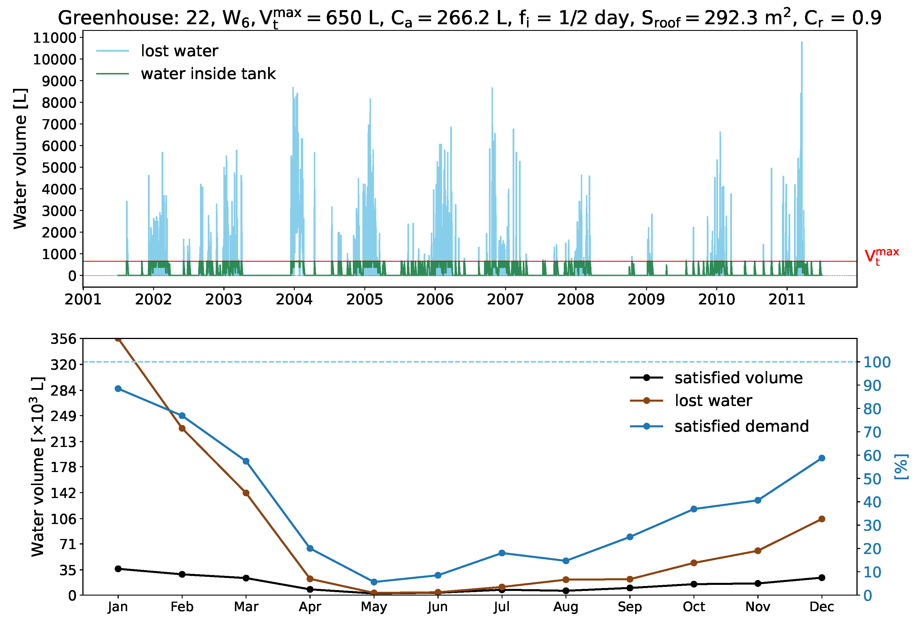
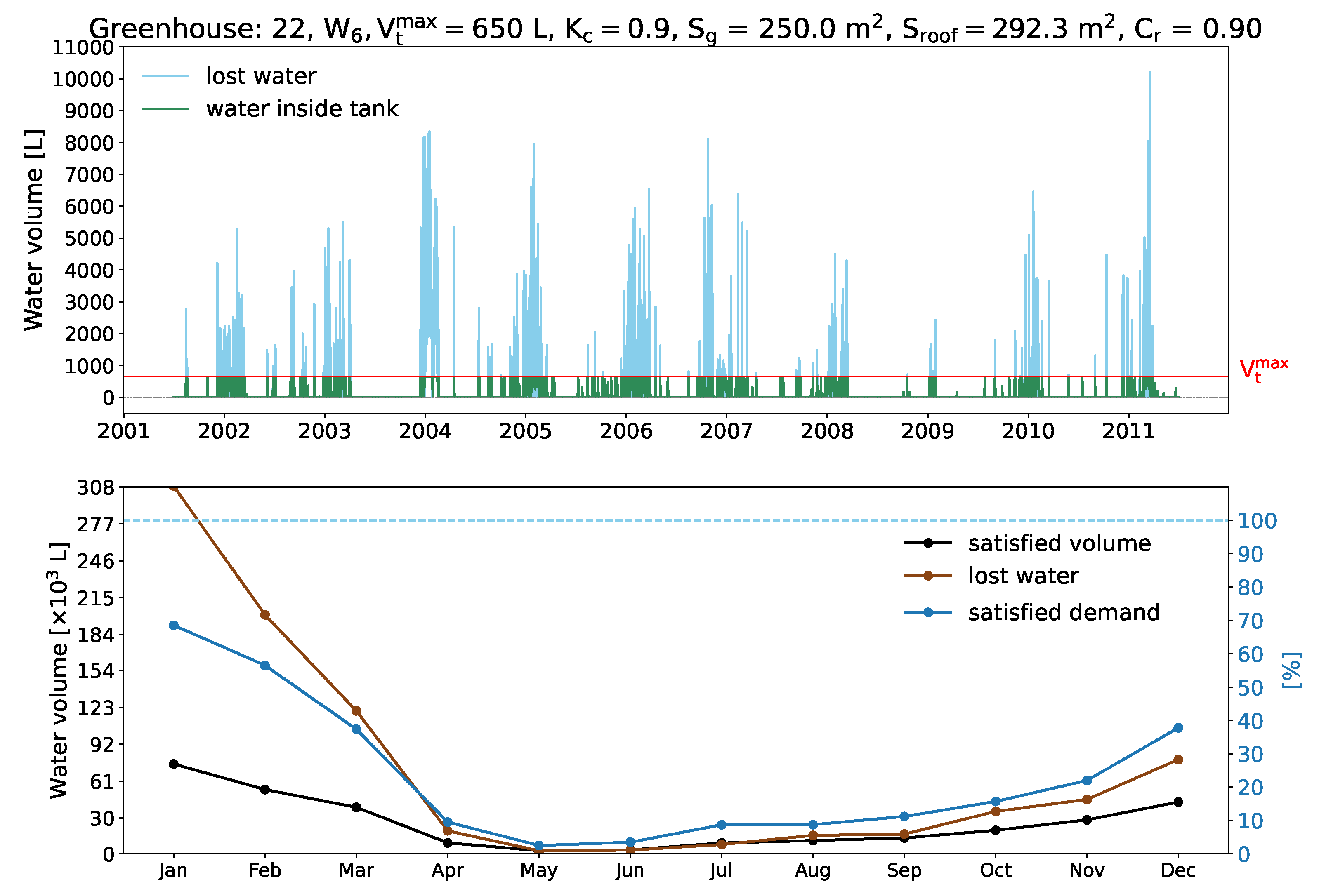
2.7. Example of Type 1 and Type 2 Simulations

As an example of Type 1 simulations performed, we show the daily volume of water inside the tank and the volume of lost water (Figure 5, top panel), as well as the 10-year monthly climatology of the percentage of satisfied water demand for greenhouse number 22 (Figure 5, bottom panel). This simulation has been performed for the following set of parameters: C r = 0.9 , W i = W 6 , f i = 1 / 2 day 1 , C a = 266.2 L, V t m a x = 650 L. As mentioned above, in this simulation, we have used the information of water irrigation provided by farmers. The daily volume of lost water (i.e., non-captured water since the tank is completely full, as indicated by the green line touching the red line), reaches peaks over 10,000 L per day during the wet season, while the tank is completely empty during most of the dry season. Note that to construct the bottom panel, daily values of satisfied demand have been first averaged at monthly scale, after which we have computed the 10-year monthly average. As seen, the satisfied demand of water for irrigation is over 60% during austral summer, while it decreases below 20% during austral winter (blue line). A similar distribution depicts the amount of water loss (red line, in thousands of liters) due to the reduced water storage (650 L). The black line represents the mean volume of water used for agriculture purposes, which in this case is always insufficient to satisfy the required volume of water for irrigation.
For comparison, we show an example of Type 2 simulations for the same greenhouse in Figure 6. It has been performed for the following set of parameters: C r = 0.9 , W i = W 6 , k c = 0.9 , S g = 250 m 2 , S r o o f = 292.3 m 2 , and V t m a x = 650 L. As seen, in this case, the mean annual cycle has the same shape than Type 1 simulations, but the percentage of satisfied water demand is about 20% smaller during the wet season (November to April) and about 10% smaller during the rest of the year. The reason is that in this case, we are irrigating every day with the theoretical water needs of crops, also assuming the greenhouse is being fully cultivated, which is not always the case in reality, since some farmers only cultivate a part of the greenhouse ground surface. On the other hand, the volume of lost water (which especially occurs during the wet season in Type 2 simulations) suggests the convenience of installing a larger tank to collect more rainwater.

3. Results and Discussions

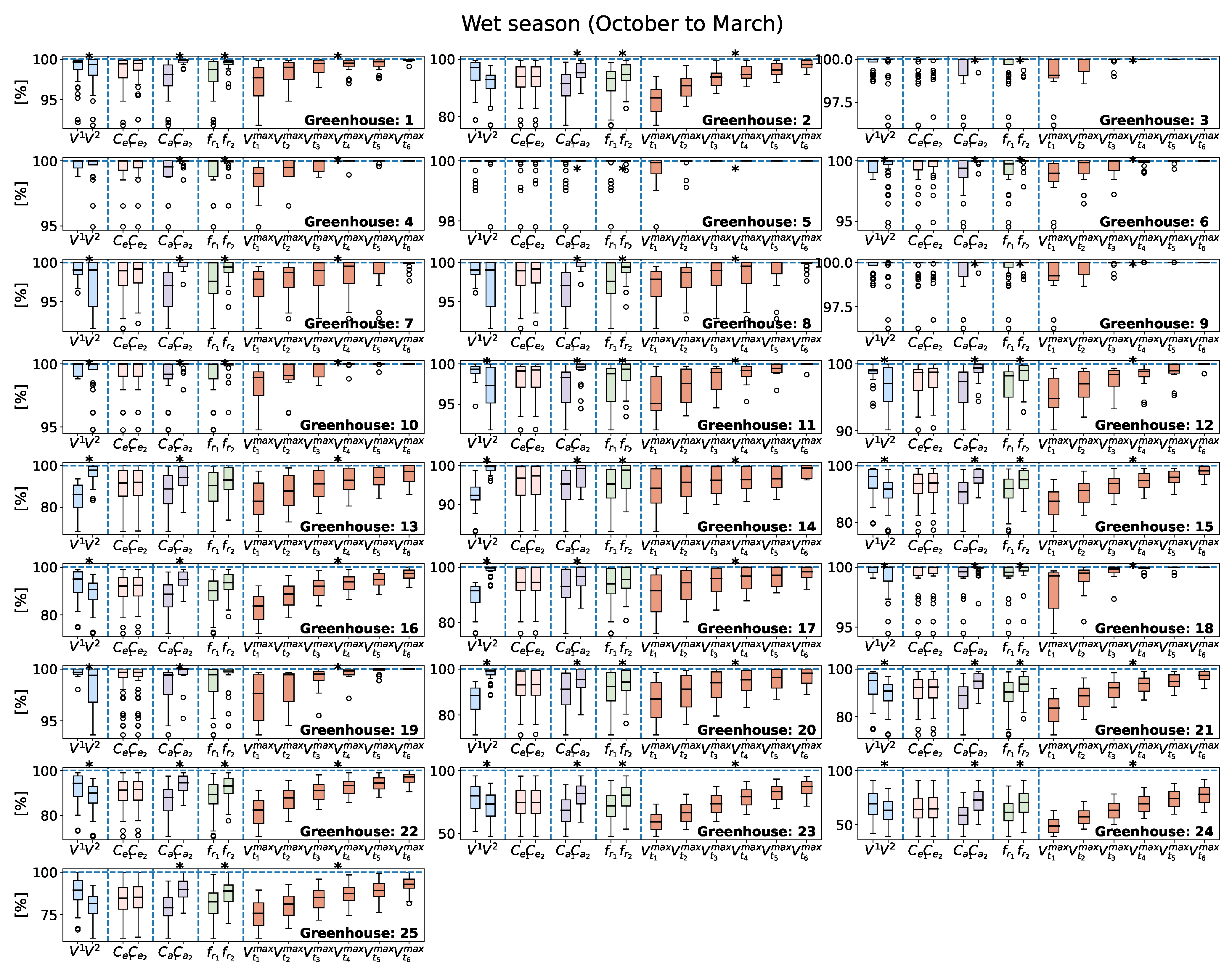
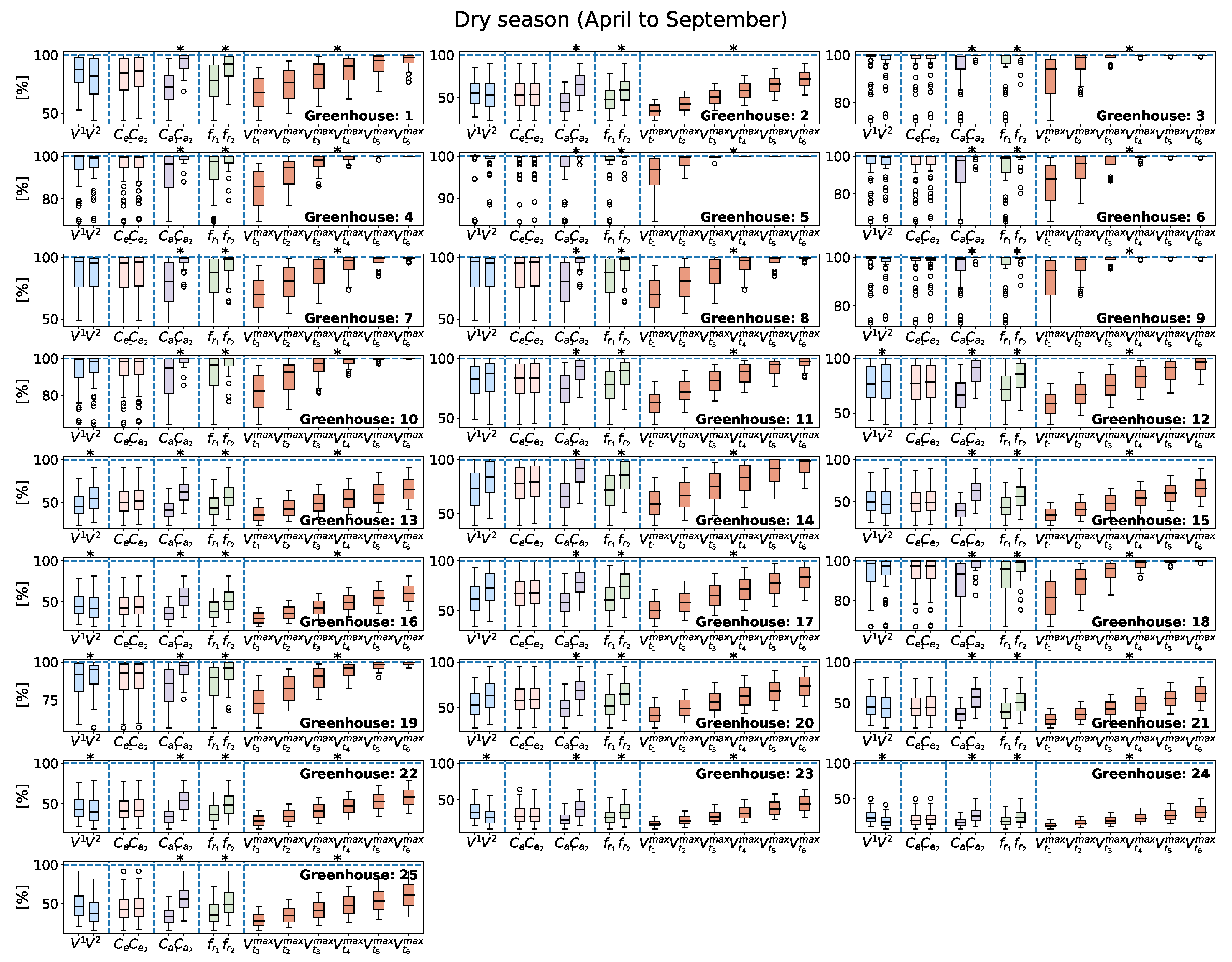
3.1. Analysis of the Satisfied Irrigation Demand According to Farmers’ Information (Type 1 Simulations)

To investigate the relevance of selected parameters in the volume of satisfied water demand in Type 1 simulations, we have compared the mean values of all simulations when one parameter is changed while the other remain fixed. Thus, the analysis is performed separately for each of the following parameters: time window ( W i , with two windows for each rain gauge as was shown in Figure 3), the runoff coefficient ( C r = 0.8 , 0.9 ), the irrigation frequency ( f i = 1 / 2 , 1 / 3 day 1 ), the volume of water used for irrigation ( C a , with two values for each greenhouse as shown in Table 2), and the maximum capacity of the tank (where V t m a x = 300 , 450 , 650 , 900 , 1200 , and 1600 L).
The obtained results for all parameters and for each greenhouse are shown in Figure 7 and Figure 8 for wet and dry seasons, respectively. Box plots include 99% of values, while those values represented as circles account for 1% of the values (outliers). The different parameters are separated by vertical dashed lines. The black horizontal line depicts the mean value, while the above asterisks indicate if for each value of every parameter, the difference between mean values is statistically significant at 95%. The significance is based on the t-test when the parameters can only take two values (which occurs for all of them except water tank capacity), and on the one-directional ANOVA (F-test) for the maximum tank capacity (only for V t m a x ), which has six case studies.
As shown in both figures, the results of satisfied water demand and their sensitivity to changes in parameters may differ between greenhouses. However, there are common characteristics to remark: (i) The average percentage of satisfied water demand varies between 50% and 100% for all study cases during the wet season and between 20 and 100% during the dry season for some combinations of parameters, being lower for greenhouses 22–25 (Table 1), which are closer to the Copancara and Corpaputo rain gauges; (ii) The percentage of satisfied water demand is statistically insensitive to the changes in the runoff coefficient here explored for all greenhouses ( C e = 0.8 , 0.9 ) and for both seasons. Mean values vary slightly for a given greenhouse (pink boxes in Figure 7 and Figure 8); (iii) Time windows have a significant effect on seven greenhouses, mainly those associated with the Huayrocondo and Copancara rain gauges (blue boxes in Figure 7 and Figure 8). The reason is that those stations have the largest difference in the number of rainy days between the two time windows selected (Table 2); (iv) The other three parameters (irrigation frequency, water volume used for irrigation, and maximum tank capacity) influence significantly at 95% over all greenhouses. Changes in irrigation frequency and volume of water used for irrigation may modify up to 20% the satisfied water demand percentage, depending on the greenhouse, while the maximum capacity of the tank can affect up to 30% the percentage of satisfied water demand, when we compare smaller with larger tanks (e.g., greenhouse 25).
The results show that if the water tank is properly selected, most of the greenhouses are able to satisfy 100% of the water demand during the wet season (greenhouses 1–21), and some of them even during the dry season (greenhouses 1, 3, 4, 5, or 6, for example), without the need of selecting the largest water tank. In contrast, greenhouses 23–24 are in trouble to reach 80% of the water demand during the wet season and 50% during the dry season. This is likely explained by the lower number of rainy days during the dry season and the large volume of water required to irrigate crops inside the greenhouse due to the large surface of their roofs.

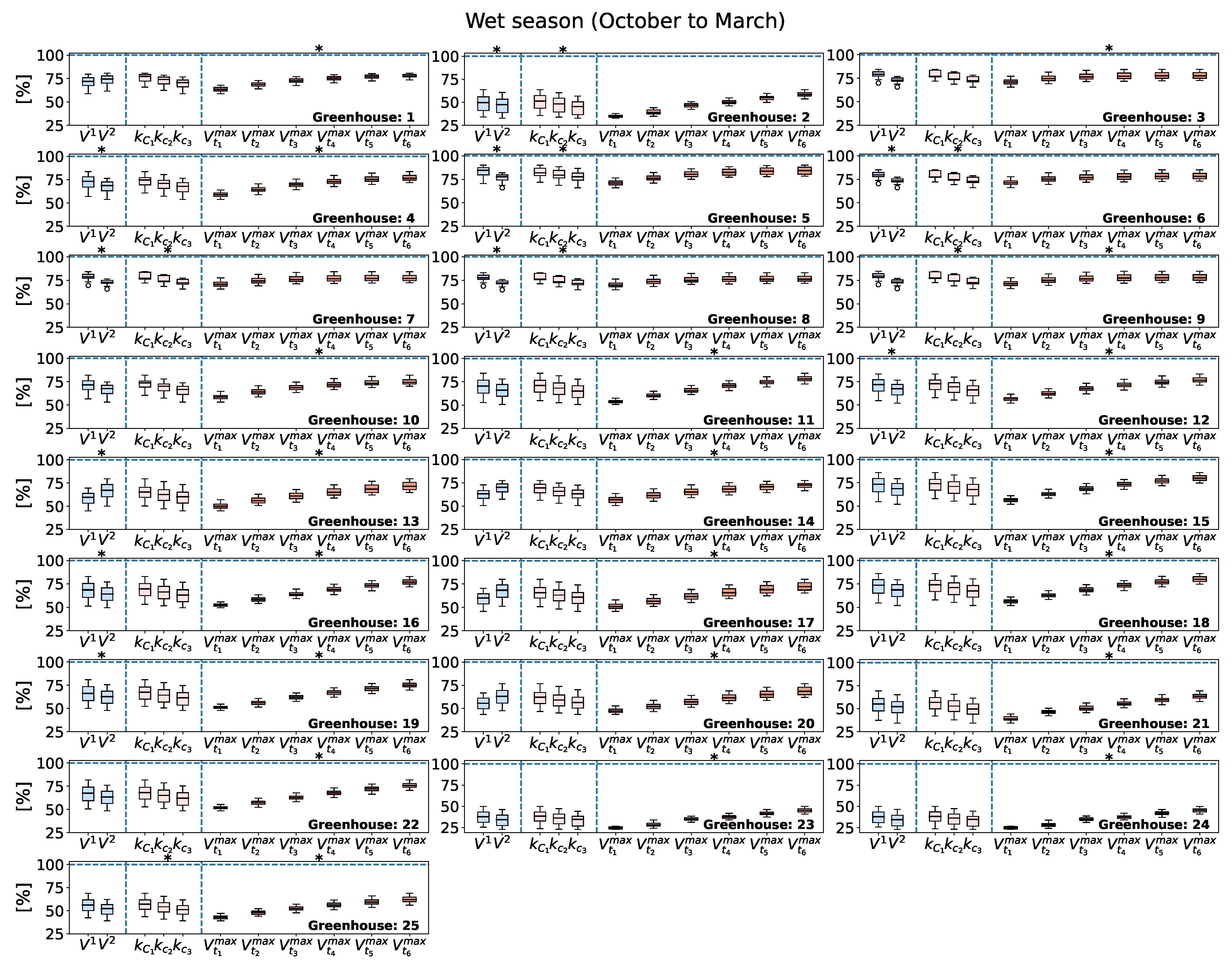
3.2. Analysis of Satisfied Irrigation Demand According to the Theoretical Crop Requirement (Type 2 Simulations)

In this section, we explore the percentage of theoretical crop total irrigation that each greenhouse with a given water tank could satisfy every day. Following the results shown above, where we verified the low sensitivity of the percentage of satisfied water demand with respect to the runoff coefficient, in Type 2 simulations, we use a constant runoff coefficient of C r = 0.9 , which is reasonable if greenhouses are properly maintained. Additionally, we explore the relevance of the crop coefficient ( k c ) by simulating three different cases: k c = 0.8 , 0.9 , 1 , as described in Section 2. As for Type 1 simulations, we also evaluate the sensitivity of results to rainfall time windows and different water tank volumes.
In this case, percentages of satisfied water demand are dramatically different between the wet and the dry seasons (Figure 9 and Figure 10, respectively), and between greenhouses. Mean percentages oscillate between 25% and 80% during the wet season and from 10% to 50% during the dry season. In many greenhouses, the percentage remains below 25% during the dry season (e.g., greenhouses 16–24). As for Type 1 simulations, significant differences between rainfall time windows appear for a few greenhouses. More interestingly, most of greenhouses where significant differences appear are distinct during the wet (2, 4–8, 12, 13, 16, and 19) and dry seasons (1, 9–11, 13–15, 17, 18, and 20–25). One explanation is that in those greenhouses with medium and large ground surface (>50 m 2 , see Table 1), rainfall differences during the dry season are larger in terms of water demand satisfaction than in the case of small size greenhouses, which with less harvested rainfall are able to satisfy their demand.
Regarding the impact of the crop coefficient in the percentage of satisfied demand, differences in the mean values are below 10% between k c = 0.8 and k c = 1 for all greenhouses. This factor is only statistically significant at 95% in greenhouses (2, 5–9, and 25) during the wet season, and in greenhouses 3, 9, and 13 during the dry seasons. All those greenhouses have a small and medium size (<50 m 2 ), being not significantly relevant the crop coefficient for large greenhouses, where the main issue is to increase the amount of harvested water.
To conclude this section, the impact of the maximum tank capacity ( V t m a x ) on the satisfied water demand reach values of up to 25 % (e.g., in greenhouse 11, Figure 9). During the wet season, the election of a certain V t m a x is significant for all greenhouses except for numbers 2 and 5–8 (Figure 9), which are the greenhouses with the lowest ground surface (<20 m 2 , Table 2). During the dry season, the volume of the tank considered in the simulation is statistically significant for all greenhouses (Figure 10), since the water is scarce and larger tanks can harvest more rainfall, thus minimizing water losses during the few isolated rainfall events.

4. Conclusions and Recommendations

In this work, we have studied the water balance between rainwater collected by greenhouse roofs and the usage of this water to irrigate crops within greenhouses if covered water tanks were available. To this end, we have followed two approaches. First, we use irrigation data collected from farmers; second, we satisfy the theoretical daily irrigation demanded by crops. We have included the most relevant parameters that affect the water balance, which are: precipitation, the runoff coefficient of greenhouse roofs, frequency and volume of irrigation, the maximum capacity of the water tank used as storage, and crop factors. Unlike other studies, which use monthly mean accumulated rainfall [36,50], here, we simulate the balance at daily scale, which better captures the impact of extreme rainfall episodes [51,52]. Our analysis has evaluated the influence of the above parameters in the percentage of satisfied water demand and the volume of water loss for each simulation type and greenhouse.
The results show that the level of irrigation carried out by farmers is far from the irrigation theoretically required in case the greenhouse was extensively cultivated. The reason is that, currently, the ground surface of many greenhouses is not being fully cultivated since farmers mostly produce for subsistence, not taking advantage of the maximum greenhouse potential. One key restriction is the current lack of water tanks, which discourage farmers from a more intensive production, since there is a real risk of water scarcity, especially during the dry season if they totally depend on rainfall or if they use flood irrigation. The greater production that farmers could get with the installation of water tanks could be sold, thus contributing to the increase of their income.
The potential effect of a degraded pipe system or the presence of sediments in the tank, which may be drawn by first waters, thus decreasing the effective volume available to store water, is small in our simulations if the reduction is 10% or lower (not shown). Two possible solutions to avoid a decrease in the volume of collected water are the installation of an auxiliary small tank for first waters or a screen to retain the biggest sediments. However, since economical resources are limited for farmers in Bolivian Altiplano, an evaluation of the economic feasibility of above solutions will be necessary to decide on the appropriate option.
Among other limitations of this study, we should cite the fact that human consumption has not been considered. This usage may exist, as in rural areas, families usually live next to greenhouses. Regarding this point, a consumption of 65 L/person/day was reported in the city of El Alto (Bolivia) a few years ago [53], which we can consider as an upper threshold for rural areas. We have not considered the degradation of greenhouse roofs (the emergence of wholes and cracks) nor critical problems in the water pipe system (e.g., obstructions), which may substantially increase water loss, and hence, reduce the volume of harvested water. The projected future changes in the volume of mean and extreme temperature and precipitation due to the ongoing climate change may also exert some impact on the results, as they have demonstrated to be sensitive to rainfall time windows for some greenhouses [54,55].
A proper maintenance of greenhouse roofs, which includes the replacement of roofs considering the polyethylene life cycle, is crucial to optimize rainwater harvesting results. This last consideration and others mentioned above related to the rainwater harvesting system require an investment of economic resources. In this sense, limited funding is another important constraint for potential users of greenhouses and rainwater harvesting systems in rural areas. It is relevant to emphasize that the institutional and public policies carried out to facilitate subsidies for productive infrastructures (greenhouses) in the highlands could increase its impact on productivity while preventing environmental threats related to the use of water for farming by promoting the installation of a well-working water harvesting system, an efficient drip irrigation system, as well as establishing a proper technical follow-up.
The information provided in this work can be used by stakeholders to decide their policies of investment in infrastructures in the Altiplano, e.g., the most optimum surface area of greenhouse roofs and water tank capacity to completely cover the water demand of crops in a certain region. Our theoretical results during the dry season (Figure 10) indicate that greenhouses 3 and 5–9 are the best options for the study area in terms of the percentage of satisfied irrigation demand. Hence, greenhouses with a small size (<50 m 2 ) are able to satisfy on average up to 50% of water requirements during the dry season if a tank of 1600 L installed. Therefore, our recommendation is the construction of greenhouses with a ground surface of between 20 and 50 m 2 , depending on the number of family members, with the largest possible covered tank volume attached (1600 L or larger if possible). We note that a smaller tank (1200 L) does not significantly impact the satisfied water demand of small greenhouses during the wet season (Figure 9), and only reduces it about 10% or less during the dry season. In those smaller greenhouses, the cultivation of crops with low water demand has a significant impact on the percentage of satisfied irrigation water (Figure 10, greenhouses 3 and 9); therefore, a proper calendar selection of crops (including an adequate planing of the crop phase) can contribute to optimize the production. As shown, the latter becomes especially critical during the dry season.
Future efforts from the public sector, NGOs, International Cooperation, and researchers regarding the implementation and evaluation of greenhouses in the Bolivian Altiplano should consider the benefits of integrating rainwater harvesting systems, which can be summarized in: (i) crop productivity improvement due to more water available for irrigation, which can be accomplished even in dry periods, depending on the design of the infrastructures and climate context of the locality; (ii) contribution to risk reduction of water depletion, mainly in areas where groundwater is used for agricultural activities, which has been warned by Satge et al. [13] as a probable consequence of intensive agriculture in the study area; and (iii) promotion of greenhouses adoption in areas where water is scarce and/or frosts are frequent. Finally, future studies aimed to assess the impact of variations in these large-scale hydrological systems should also consider the reduction of river flow and the slower recharge of groundwater sources by runoff.

Author Contributions

Conceptualization, J.-M.S.; methodology, J.-M.S. and V.A.; formal analysis, J.-M.S.; data curation, J.-M.S., V.A., and C.E.Q.; visualization, J.-M.S.; writing—original draft preparation, J.-M.S.; writing—review and editing, J.-M.S., V.A., C.E.Q., I.V., and J.-P.B.L.; supervision, J.-P.B.L.; funding acquisition, I.V. All authors have read and agreed to the published version of the manuscript.

Funding

This research has been funded by Generalitat Valenciana.

Institutional Review Board Statement

Not applicable.

Informed Consent Statement

Not applicable.

Data Availability Statement

Codes and greenhouses data of this study are available from the corresponding author on reasonable request. Rainfall time series are available from SENAMHI under written request at https://senamhi.gob.bo/index.php/guia (accessed on 13 April 2022). We use CPC Global Temperature data are provided by the NOAA/OAR/ESRL PSL, Boulder, CO, USA, and is freely downloadable from their website at https://psl.noaa.gov/data/gridded/data.cpc.globaltemp.html (accessed on 13 April 2022).

Acknowledgments

J.-M.S thanks the financial support by Generalitat Valenciana and the European Social Fund (ESF) through the APOSTD/2020/254 grant. All authors thank funding from Generalitat Valenciana, Consellería de Participación, Transparencia, Cooperación y Calidad democrática, and from the University of Alicante, Vicerrectorado de Relaciones Internacionales y Cooperación para el Desarrollo. J.-M.S., V.A., C.E.Q., and J.-P.B.L. acknowledge support from the project “Pequeños Proyectos de Investigación” to the awarded project: “¿Son los invernaderos socioeconómica y ambientalmente sostenibles? Evaluación diagnóstico para optimizar la eficiencia de uso de agua y aprovechar el potencial productivo de los invernaderos instalados en el municipio de Batallas”, funded by Universidad Católica Boliviana San Pablo-La Paz.

Conflicts of Interest

The authors have no relevant financial or non-financial interests to disclose. The content of this publication is only responsibility of the University of Alicante, and does not necessarily reflects the opinion of Generalitat Valenciana.

References

  1. Ramírez, E.; Francou, B.; Ribstein, P.; Descloitres, M.; Guérin, R.; Mendoza, J.; Gallaire, R.; Pouyaud, B.; Jordan, E. Small glaciers disappearing in the tropical Andes: A case-study in Bolivia: Glaciar Chacaltaya (16° S). J. Glaciol. 2001, 47, 187–194. [Google Scholar] [CrossRef] [Green Version]
  2. Lee, C.C. Weather whiplash: Trends in rapid temperature changes in a warming climate. Int. J. Climatol. 2021, 42, 4214–4222. [Google Scholar] [CrossRef]
  3. Masiokas, M.H.; Rabatel, A.; Rivera, A.; Ruiz, L.; Pitte, P.; Ceballos, J.L.; Barcaza, G.; Soruco, A.; Bown, F.; Berthier, E.; et al. A Review of the Current State and Recent Changes of the Andean Cryosphere. Front. Earth Sci. 2020, 8, 99. [Google Scholar] [CrossRef]
  4. Thibeault, J.M.; Seth, A.; Garcia, M. Changing climate in the Bolivian Altiplano: CMIP3 projections for temperature and precipitation extremes. J. Geophys. Res. Atmos. 2010, 115, 1–18. [Google Scholar] [CrossRef]
  5. Seiler, C.; Hutjes, R.W.A.; Kabat, P. Likely Ranges of Climate Change in Bolivia. J. Appl. Meteorol. Climatol. 2013, 52, 1303–1317. [Google Scholar] [CrossRef]
  6. Andrade, M.F. (Ed.) Atlas-Clima y Eventos Extremos del Altiplano Central perú-Boliviano/Climate and Extreme Events from the Central Altiplano of Peru and Bolivia 1981–2010; Geographica Bernensia: Bern, Switzerland, 2018; p. 118. [Google Scholar] [CrossRef]
  7. Soruco, A.; Vincent, C.; Rabatel, A.; Francou, B.; Thibert, E.; Sicart, J.E.; Condom, T. Contribution of glacier runoff to water resources of La Paz city, Bolivia (16° S). Ann. Glaciol. 2015, 56, 147–154. [Google Scholar] [CrossRef] [Green Version]
  8. Rangecroft, S.; Harrison, S.; Anderson, K. Rock Glaciers as Water Stores in the Bolivian Andes: An Assessment of Their Hydrological Importance. Arct. Antarct. Alp. Res. 2015, 47, 89–98. [Google Scholar] [CrossRef] [Green Version]
  9. Cook, S.J.; Kougkoulos, I.; Edwards, L.A.; Dortch, J.; Hoffmann, D. Glacier change and glacial lake outburst flood risk in the Bolivian Andes. Cryosphere 2016, 10, 2399–2413. [Google Scholar] [CrossRef] [Green Version]
  10. Garcia, M.; Raes, D.; Jacobsen, S.E.; Michel, T. Agroclimatic constraints for rainfed agriculture in the Bolivian Altiplano. J. Arid. Environ. 2007, 71, 109–121. [Google Scholar] [CrossRef]
  11. Vicente-Serrano, S.; Kenawy, A.E.; Azorin-Molina, C.; Chura, O.; Trujillo, F.; Aguilar, E.; Martín-Hernández, N.; López-Moreno, J.; Sanchez-Lorenzo, A.; Moran-Tejeda, E.; et al. Average monthly and annual climate maps for Bolivia. J. Maps 2016, 12, 295–310. [Google Scholar] [CrossRef] [Green Version]
  12. Canedo-Rosso, C.; Uvo, C.B.; Berndtsson, R. Precipitation variability and its relation to climate anomalies in the Bolivian Altiplano. Int. J. Climatol. 2019, 39, 2096–2107. [Google Scholar] [CrossRef] [Green Version]
  13. Satgé, F.; Ruelland, D.; Bonnet, M.P.; Molina, J.; Pillco, R. Consistency of satellite-based precipitation products in space and over time compared with gauge observations and snow-hydrological modelling in the Lake Titicaca region. Hydrol. Earth Syst. Sci. 2019, 23, 595–619. [Google Scholar] [CrossRef] [Green Version]
  14. Miranda, G.; Chávez, R.; Argollo, J.; Figueroa, F. Dinamica de las precipitaciones pliviales en el Altiplano Boliviano. In Simposio Nacional de Cambios Globales; Argollo, J., Miranda, G., Eds.; Centro Investigaciones Cambios Globales: La Paz, Bolivia, 2000; pp. 56–67. [Google Scholar]
  15. François, C.; Bosseno, R.; Vacher, J.; Seguin, B. Frost risk mapping derived from satellite and surface data over the Bolivian Altiplano. Agric. For. Meteorol. 1999, 95, 113–137. [Google Scholar] [CrossRef]
  16. Buxton, N.; Escobar, M.; Purkey, D.; Lima, N. Water Scarcity, Climate Change and Bolivia: Planning for Climate Uncertainties; Technical Report; Stockholm Environment Institute: Stockholm, Sweden, 2013. [Google Scholar]
  17. Seiler, C.; Hutjes, R.W.A.; Kabat, P. Climate Variability and Trends in Bolivia. J. Appl. Meteorol. Climatol. 2013, 52, 130–146. [Google Scholar] [CrossRef] [Green Version]
  18. Canedo-Rosso, C.; Hochrainer-Stigler, S.; Pflug, G.; Condori, B.; Berndtsson, R. Drought impact in the Bolivian Altiplano agriculture associated with the El Niño–Southern Oscillation using satellite imagery data. Nat. Hazards Earth Syst. Sci. 2021, 21, 995–1010. [Google Scholar] [CrossRef]
  19. Tito, C.; Wanderley, F. Contribución de la Agricultura Familiar Campesina e Indígena a la Producción y Consumo de Alimentos en Bolivia, 1st ed.; CIPCA: La Paz, Bolivia, 2021; p. 137. [Google Scholar]
  20. INE. Encuesta Agropecuaria 2015; Technical Report; Instituto Nacional de Estadística: La Paz, Bolivia, 2017. [Google Scholar]
  21. Urioste, M. Concentration and “foreignisation” of land in Bolivia. Can. J. Dev. Stud. 2012, 33, 439–457. [Google Scholar] [CrossRef]
  22. Winkel, T.; Alvarez-Flores, R.; Bommel, P.; Bourliaud, J.; Chevarria Lazo, M. The Southern Altiplano of Bolivia. State of the Art Report on Quinoa around the World in 2013; Food and Agriculture Organization of the United Nations: Rome, Italy, 2018; p. 589. [Google Scholar]
  23. FAO. El Alto; Technical Report; Organización de las Naciones Unidas para la Alimentación y la Agricultura: Roma, Italy, 2014. [Google Scholar]
  24. Torrico Albino, J.C. Desarrollo Rural y Agroalimentario en Bolivia: Procesos, Problemática y Perspectivas, 1st ed.; ePubli: Cologne, Germany, 2014; p. 333. [Google Scholar]
  25. Gianotten, V. CIPCA y Poder Campesino Indígena. 35 años de Historia, 1st ed.; CIPCA: La Paz, Bolivia, 2006; p. 412. [Google Scholar]
  26. Pérez Mamani, V. (Ed.) Beneficios de los Sistemas Agroecológicos Familiares en el Altiplano, 1st ed.; CIPCA: La Paz, Bolivia, 2021; p. 238. [Google Scholar]
  27. MDRyT. Plan del Sector Agropecuario y Rural con Desarrollo Integral Para Vivir Bien-PSARDI; Technical Report; Ministerio de Desarrollo Rural y Tierras: La Paz, Bolivia, 2017. [Google Scholar]
  28. FAO. Carpas Solares de Hampaturi en Plena Producción; Technical Report; Food and Agriculture Organization: Roma, Italy, 2015. [Google Scholar]
  29. MMAyA. Más de Mil Millones de Bolivianos en Inversión en Proyectos de Agua a Nivel Nacional; Technical Report; Ministerio de Medio Ambiente y Agua: La Paz, Bolivia, 2021. [Google Scholar]
  30. MDRyT. Inversión Histórica: Gobierno Nacional Aprueba Presupuesto Para Fortalecer la Producción Agrícola Urbana y Periurbana; Technical Report; Ministerio de Desarrollo Rural y Tierras: La Paz, Bolivia, 2021. [Google Scholar]
  31. Doss, C.R. Analyzing technology adoption using microstudies: Limitations, challenges, and opportunities for improvement. Agric. Econ. 2006, 34, 207–219. [Google Scholar] [CrossRef]
  32. Mariano, M.J.; Villano, R.; Fleming, E. Factors influencing farmers’ adoption of modern rice technologies and good management practices in the Philippines. Agric. Syst. 2012, 110, 41–53. [Google Scholar] [CrossRef]
  33. Mugambi, D.M. Factors Influencing the Adoption of Greenhouse Farming by Smallholders in Central Imenti Subcounty in Meru County. Master’s Thesis, University of Nairobi, Nairobi, Kenya, 2020. [Google Scholar]
  34. Muriithi, D.I.; Wambua, B.N.; Omoke, K.J. Constraints and Opportunities for Greenhouse Farming Technology as an Adaptation Strategy to Climate Variability by Smallholder Farmers of Nyandarua County of Kenya. East Afr. J. Sci. Technol. Innov. 2021, 2, 1–13. [Google Scholar]
  35. Gossweiler, B.; Wesström, I.; Messing, I.; Romero, A.M.; Joel, A. Spatial and Temporal Variations in Water Quality and Land Use in a Semi-Arid Catchment in Bolivia. Water 2019, 11, 2227. [Google Scholar] [CrossRef] [Green Version]
  36. Aladenola, O.O.; Adeboye, O.B. Assessing the Potential for Rainwater Harvesting. Water Resour. Manag. 2010, 24, 2129–2137. [Google Scholar] [CrossRef]
  37. Clifford, A. Multivariate Error Analysis: A Handbook of Error Propagation and Calculation in Many-Parameter Systems; John Wiley & Sons: Hoboken, NJ, USA, 1973. [Google Scholar]
  38. Imteaz, M.A.; Shanableh, A.; Rahman, A.; Ahsan, A. Optimisation of rainwater tank design from large roofs: A case study in Melbourne, Australia. Resour. Conserv. Recycl. 2011, 55, 1022–1029. [Google Scholar] [CrossRef]
  39. Kakoulas, D.A.; Golfinopoulos, S.K.; Koumparou, D.; Alexakis, D.E. The Effectiveness of Rainwater Harvesting Infrastructure in a Mediterranean Island. Water 2022, 14, 716. [Google Scholar] [CrossRef]
  40. Thomas, T.H.; Martinson, D.B. Roofwater Harvesting: A Handbook for Practitioners; Technical Report Technical Paper Series; IRC International Water and Sanitation Centre: Delft, The Netherlands, 2007. [Google Scholar]
  41. Ishaku, H.T.; Majid, M.R.; Johar, F. Rainwater Harvesting: An Alternative to Safe Water Supply in Nigerian Rural Communities. Water Resour. Manag. 2012, 26, 295–305. [Google Scholar] [CrossRef] [Green Version]
  42. Hargreaves, G.H.; Samani, Z. Reference Crop Evapotranspiration from Temperature. Appl. Eng. Agric. 1985, 1, 96–99. [Google Scholar] [CrossRef]
  43. Vicente-Serrano, S.M.; Chura, O.; López-Moreno, J.I.; Azorin-Molina, C.; Sanchez-Lorenzo, A.; Aguilar, E.; Moran-Tejeda, E.; Trujillo, F.; Martínez, R.; Nieto, J.J. Spatio-temporal variability of droughts in Bolivia: 1955–2012. Int. J. Climatol. 2015, 35, 3024–3040. [Google Scholar] [CrossRef] [Green Version]
  44. Pereira, L.S.; Allen, R.G.; Smith, M.; Raes, D. Crop evapotranspiration estimation with FAO56: Past and future. Agric. Water Manag. 2015, 147, 4–20. [Google Scholar] [CrossRef]
  45. Choueiter, D.; Farajalla, N. National Guidelines for Greenhouse Rainwater Harvesting Systems in the Agriculture Sector; Technical Report; Ministry of Environment and United Nations Development Programme: Beirut, Lebanon, 2016. [Google Scholar]
  46. Nikolaou, G.; Neocleous, D.; Katsoulas, N.; Kittas, C. Irrigation of Greenhouse Crops. Horticulturae 2019, 5, 7. [Google Scholar] [CrossRef] [Green Version]
  47. Allen, R.G.; Pereira, L.S.; Raes, D.; Smith, M. Crop Evapotranspiration-Guidelines for Computing Crop Water Requirements-FAO Irrigation and Drainage Paper 56; Technical Report; FAO-Food and Agriculture Organization of the United Nations: Rome, Italy, 1998. [Google Scholar]
  48. Ghisi, E.; da Fonseca Tavares, D.; Rocha, V.L. Rainwater harvesting in petrol stations in Brasília: Potential for potable water savings and investment feasibility analysis. Resour. Conserv. Recycl. 2009, 54, 79–85. [Google Scholar] [CrossRef]
  49. Farreny, R.; Morales-Pinzón, T.; Guisasola, A.; Tayà, C.; Rieradevall, J.; Gabarrell, X. Roof selection for rainwater harvesting: Quantity and quality assessments in Spain. Water Res. 2011, 45, 3245–3254. [Google Scholar] [CrossRef]
  50. Lupia, F.; Baiocchi, V.; Lelo, K.; Pulighe, G. Exploring Rooftop Rainwater Harvesting Potential for Food Production in Urban Areas. Agriculture 2017, 7, 46. [Google Scholar] [CrossRef] [Green Version]
  51. Rowe, M.P. Rain Water Harvesting in Bermuda. J. Am. Water Resour. Assoc. 2011, 47, 1219–1227. [Google Scholar] [CrossRef]
  52. Londra, P.A.; Kotsatos, I.E.; Theotokatos, N.; Theocharis, A.T.; Dercas, N. Reliability Analysis of Rainwater Harvesting Tanks for Irrigation Use in Greenhouse Agriculture. Hydrology 2021, 8, 132. [Google Scholar] [CrossRef]
  53. Red-Hábitat. Gestión Integral del Agua. Available online: https://cambioclimatico-bolivia.org/archivos/20120806044617_0.pdf (accessed on 4 October 2021).
  54. Marengo, J.A.; Jones, R.; Alves, L.M.; Valverde, M.C. Future change of temperature and precipitation extremes in South America as derived from the PRECIS regional climate modeling system. Int. J. Climatol. 2009, 29, 2241–2255. [Google Scholar] [CrossRef] [Green Version]
  55. Cabré, M.F.; Solman, S.; Núñez, M. Regional climate change scenarios over southern South America for future climate (2080–2099) using the MM5 Model. Mean, interannual variability and uncertainties. Atmósfera 2016, 29, 35–60. [Google Scholar] [CrossRef] [Green Version]
Figure 1. (a) Map of South America with Bolivia highlighted. (b) Map of Bolivia with Batallas Municipality detailed. (c) Altitude map of Batallas Municipality and surroundings. Greenhouses are depicted by triangles (even or two slopes roof), semi circles (semi-spherical roof), and squares (single slope roof). The closest rain gauges with at least 20 years of daily rainfall measurements are depicted with circles. Note that colors of greenhouses and the closest weather station are the same. Daily temperature location is depicted by a black star. The distance of each greenhouse to the closest rain gauge is shown in Table 1.
Hydrology 09 00107 g001
Figure 2. Photographs illustrating the different greenhouse roof types used by local farmers: (a) two slopes, (b) semi spherical, (c) single slope. These images correspond to greenhouses 1, 22, and 25, respectively (see their characteristics in Table 1).
Hydrology 09 00107 g002
Figure 3. Time series of rainfall from the closest weather stations to greenhouses (Figure 1): Chirapaca (pink circle), Huayrocondo (green circle), Copancara (blue circle), and Corpaputo (red circle). For each time series, we have chosen two time windows that span 10 years and do not overlap with each other (rectangles, named as W i , i = 1 8 ). Note that one window starts in summer and another one in winter (Table 2).
Hydrology 09 00107 g003
Figure 4. (a) Time series of maximum ( T max ), minimum ( T min ), and mean ( T ¯ ) daily temperature (unit of °C). Time series correspond to the coordinates: [ 68.5 ° W, 16.25 ° S]. (b) Time series of daily reference crop evapotranspiration, ET 0 (unit of L · m 2 · day 1 ).
Hydrology 09 00107 g004
Figure 5. Example of a Type 1 simulation performed with Equation (2) for greenhouse 22 (see main characteristics in Table 1). The simulation is performed for the next set of parameters: S r o o f = 292.3 m 2 , C r = 0.9 , W i = W 6 (second window of Copancara station, Table 1), f i = 1 / 2 day , C a = 266.2 L, V t m a x = 650 L. (top panel) Daily simulation of water inside tank (green) and lost water (sky blue). Note that the amount of water inside the tank is V t m a x as maximum. (bottom panel) The 10-year monthly mean computed from daily data. The percentage of satisfied demand (sky blue) has been calculated taking into account the volume of water provided by the tank (black) with respect to the total required, while the water loss (brown) indicates the amount of water does not captured, most likely due to limitations in the storage capacity of the tank. Units of left y-axis are 10 3 L.
Hydrology 09 00107 g005
Figure 6. Example of a Type 2 simulation performed with Equation (3) for greenhouse 22 (see the main characteristics in Table 2). The simulation is performed for the next set of parameters: S r o o f = 292.3 m 2 , C r = 0.9 , W i = W 6 (second window of Copancara station, Table 2), k c = 0.9 , S g = 250 m 2 , V t m a x = 650 L. (top panel) Daily simulation of water inside tank (green) and lost water (sky blue). Note that the amount of water inside the tank is V t m a x as maximum. (bottom panel) The 10-year monthly mean computed from daily data. The percentage of satisfied demand (sky blue) has been calculated taking into account the volume of water provided by the tank (black) with respect to the total required, while the water loss (brown) indicates the amount of water does not captured, most likely due to limitations in the storage capacity of the tank. Units of the left y-axis are 10 3 L.
Hydrology 09 00107 g006
Figure 7. Box plots of the mean percentage of satisfied water demand during the wet season, October to March (y-axis) for each greenhouse and for each parameter included in Type 1 simulations. Note that box plots reflect changes when one parameter is modified while the other remain fixed. The parameters are: 10-year time window of rainfall ( W 1 o W 2 depending on the beginning of time series, summer or winter, according to Table 2) depicted by blue boxes; the runoff coefficient ( C r 1 = 0.8 , C r 2 = 0.9 , depicted by pink boxes); the water needed for irrigation, which depends on the number of irrigation drips and the greenhouse size, as well as on the frequency of irrigation and on the duration of each irrigation event, presenting two scenarios: larger water usage ( C a 1 ) or lower water usage ( C a 2 ) depicted by purple boxes; the irrigation frequency, once every two days ( f i 1 = 1 / 2 day 1 ) or once every three days ( f i 2 = 1 / 3 day 1 ), depicted by green boxes; and the maximum capacity of water tanks: 300 L, 450 L, 650 L, 900 L, 1200 L, and 1600 L, depicted by orange boxes. Note that each parameter is separated by vertical dashed lines. The statistical significance of obtained values for the different set of parameters has been calculated using a t-test when we compare two factors, and through an ANOVA one-directional (F-test) when the number of factors is larger than two, which only occurs for the maximum capacity of the tank ( V t i m a x ). The black asterisks that sometimes appear above box plots indicate when the difference between the means is significant at 95%, i.e., p v a l u e 0.05 .
Hydrology 09 00107 g007
Figure 8. Same as Figure 7 but for the dry season (April to September).
Hydrology 09 00107 g008
Figure 9. Box plots of the mean percentage of satisfied water demand during the wet season, October to March (y-axis) for each greenhouse and for each parameter included in Type 2 simulations. Note that box plots reflect changes when one parameter is modified while the others remain fixed. The parameters are: 10-year time window of rainfall ( W 1 or W 2 , depending on the beginning of time series, summer or winter, according to Table 2) depicted by blue boxes; the crop coefficient ( k c 1 = 0.8 , k c 2 = 0.9 , k c 3 = 1 ), depicted by pink boxes; and the maximum capacity of water tanks: 300 L, 450 L, 650 L, 900 L, 1200 L, and 1600 L, depicted by orange boxes. For all simulations, the runoff coefficient is fixed ( C r = 0.9 ). Note that each parameter is separated by vertical dashed lines. The statistical significance of obtained values for the different set of parameters has been calculated using a t-test when we compare two factors, and through an ANOVA one-directional (F-test) when the number of factors is larger than two, which occurs for the crop coefficient ( k c i ) and the maximum capacity of the tank ( V t i m a x ). The black asterisks that sometimes appear above box plots indicate when the difference between the means is significant at 95%, i.e., p v a l u e 0.05 .
Hydrology 09 00107 g009
Figure 10. Same as Figure 9 but for the dry season (April to September).
Hydrology 09 00107 g010
Table 1. Position, greenhouse ground surface, catchment surface, closest rain gauge, and distance, as well as volume of water used for irrigation for the two types of irrigation drips.
GreenhousePositionGreenhouse Surface (m2)Closest Rain GaugeDistance (km)Catchment Surface (m2)Ca [L]
1(16.266 ° S, 68.475 ° W)261.3Chirapaca0.4300.0(156.96, 77.76)
2(16.269 ° S, 68.470 ° W)19.3Chirapaca4.322.0(11.88, 5.58 )
3(16.272 ° S, 68.470 ° W)49.5Chirapaca4.457.3(18.30, 8.91 )
4(16.272 ° S, 68.470 ° W)29.3Chirapaca4.446.2(9.90, 4.77)
5(16.272 ° S, 68.459 ° W)19.3Chirapaca4.422.4(14.65, 6.88)
6(16.260 ° S, 68.456 ° W)18.4Chirapaca6.220.5(23.04, 10.80)
7(16.261 ° S, 68.459 ° W)18.9Chirapaca6.320.5(23.04, 10.80)
8(16.258 ° S, 68.499 ° W)18.4Chirapaca6.321.1(11.52, 5.40)
9(16.307 ° S, 68.465 ° W)44Chirapaca0.946.1(19.80, 9.68)
10(16.292 ° S, 68.482 ° W)89.3Chirapaca3.8140.1(47.52, 23.40)
11(16.281 ° S, 68.544 ° W)60.0Chirapaca2.772.0(49.14, 23.94)
12(16.338 ° S, 68.475 ° W)80.3Huayrocondo5.1126.0(125.82, 61.83 )
13(16.335 ° S, 68.571 ° W)35.0Huayrocondo8.038.8(34.63, 16.87)
14(16.316 ° S, 68.546 ° W )75.0Chirapaca5.6118.5(138.24, 68.04)
15(16.305 ° S, 68.546 ° W)100.0Chirapaca5.4158.0(181.44, 89.64)
16(16.323 ° S, 68.546 ° W)75.0Huayrocondo5.8118.5(69.12, 34.02)
17(16.308 ° S, 68.552 ° W)75.0Chirapaca6.0118.5(23.04, 11.34)
18(16.308 ° S, 68.552 ° W)113.9Chirapaca6.0178.0(32.76, 16.17)
19(16.348 ° S, 68.571 ° W)106.2Huayrocondo8.0167.4(105.23, 51.95)
20(16.308 ° S, 68.524 ° W)168.0Chirapaca3.0178.3(184.70, 91.46)
21(16.319 ° S, 68.519 ° W)108.0Chirapaca3.2169.2(199.08, 98.28)
22(16.258 ° S, 68.568 ° W)250.0Copancara2.1292.3(266.18, 131.87)
23(16.262 ° S, 68.561 ° W)255.0Copancara2.6306.0(441.54, 218.79)
24(16.259 ° S, 68.567 ° W)57.5Copancara2.267.3(100.44, 49.14)
25(16.019 ° S, 68.517 ° W )39.2Corpaputo6.439.6(51.84, 24.84)
Table 2. Main characteristics of rainfall for selected time windows ( W 1 , , W 8 ). There are two windows that span 10 years for each rain gauge, one beginning in austral summer and another one in winter, respectively. Maximum daily rainfall, the total 10-year accumulated rainfall, and the percentage of rainy days are included for each time window.
WindowsRain GaugeCoverageDaily Max. (mm)Total Rainfall (mm)% of Rainy Days
W 1 Chirapaca1 January 1992–31 December 200140.05703.325.4 %
W 2 Chirapaca1 July 2004–30 June 201430.05020.823.2 %
W 3 Huayrocondo1 January 1992–31 December 200140.64869.522.8 %
W 4 Huayrocondo1 July 2004–30 June 201437.45186.730.5 %
W 5 Copancara1 January 1990–31 December 1999374323.516.8 %
W 6 Copancara1 July 2001–30 June 201142.04589.814.0 %
W 7 Corpaputo1 January 1981–31 December 199032.97149.734.3 %
W 8 Corpaputo1 July 1992–30 June 200223.26769.832.1 %
Publisher’s Note: MDPI stays neutral with regard to jurisdictional claims in published maps and institutional affiliations.

