
Measuring and Modelling Evaporation Losses from Wet Branches of Lemon Trees


Department of Agricultural, Food and Forest Sciences (SAAF), University of Palermo, Viale delle Scienze, Bldg 4, 90128 Palermo, Italy
*
Author to whom correspondence should be addressed.
Hydrology 2022, 9(7), 118; https://0-doi-org.brum.beds.ac.uk/10.3390/hydrology9070118
Submission received: 31 May 2022
/
Revised: 23 June 2022
/
Accepted: 25 June 2022
/
Published: 28 June 2022
Abstract
:Evaporation losses of rainfall intercepted by canopies depend on many factors, including the temporal scale of observations. At the event scale, interception is a few millimetres, whereas at a larger temporal scale, the number of times that a canopy is filled by rainfall and then depleted can make the interception an important fraction of the rainfall depth. Recently, a simplified interception/evaporation model has been proposed, which considers a modified Merrian model to compute interception during wet spells and a simple power-law equation to model evaporation from wet canopy during dry spells. Modelling evaporation process at the sub hourly temporal scale required the two parameters of the power-law, describing the hourly evaporation depth and the evaporation rate. In this paper, for branches of lemon trees, we focused on the evaporation process from wet branches starting from the interception capacity, S, and simple models in addition to the power-law were applied and tested. In particular, for different temperature, T, and vapour pressure deficit, VPD, conditions, numerous experimental testes were carried out, and the two parameters describing the evaporation process from wet branches were determined and linked to T, VPD and S. The results obtained in this work help us to understand the studied process, highlight its complexity, and could be implemented in the recently introduced interception/evaporation model to quantify this important component of the hydrologic cycle.
1. Introduction
Interception loss is a part of rainfall that is intercepted by the Earth’s surface and subsequently evaporates [1]. From a hydrological point of view, where more emphasis is given to the related hydrological processes, interception loss is defined as a part of rainfall that is mostly captured by vegetation, and it cannot take part in the runoff and infiltration processes, since it is bound to evaporate [2,3]. The role of interception in the hydrologic cycle has probably been underestimated and sometimes completely neglected [4]. Beven [5] stated that in some environments, evaporation from intercepted water via wet and rough canopies can be very significant in the total water balance. Calder [6] showed that in the upland forest catchments of Britain, evaporation from interception amounted to 35% of the gross rainfall in areas where more than 1000 mm of annual rainfall occurred. However, in areas with lower rainfall and high vegetation cover, evaporation from interception can be more significant, achieving 40–50% of the gross rainfall [4]. For a number of different environments and species, Carlyle-Moses [7] also stated that interception loss is often an important component of water balance and found that, on average, it was equal to 26 and 13% of the gross precipitation for coniferous and foliated deciduous forests, respectively. Therefore, the need to develop parsimonious simple models able to predict this component of the hydrological cycle, which require few parameters and can be applied at a large scale, is widely acknowledged [8], especially for orchards where it seems that less experimental research was carried out than for forests.
The increased interest in the potential of tree planting to help mitigate flooding, increase the soil infiltration capacity [9], enhance soil drying resulting from transpiration and wet-canopy evaporation, increase ground-surface roughness and also reduce the splash and surface erosion caused by raindrop impacts [10], encouraged us to pursue a deeper understanding of the interception process. For low rainfall intensities, and consequently for small drop sizes, which are more frequent at the yearly scale, it is reasonable to accept that interception plays a crucial role in the hydrologic cycle [10,11]. However, for extreme rainfall events, it was also shown that the importance of vegetation cover decreases [12].
Of course, in irrigation, when sprinklers are applied under limited water application rates, interception also affects the water balance. For example, Jiao et al. [13] developed a process-based dynamic interception model for alfalfa canopies, validated it under conditions of simulated sprinkler irrigation and demonstrated that the amount of interception increased rapidly with duration in the early stage of sprinkler irrigation and then gradually levelled off until the maximum retention capacity of the canopy was reached.
The most commonly applied interception models are described in a review article by Muzylo et al. [14], who listed the peculiarities of each model, also indicating the required input temporal scale, the output variables, the number of parameters, the number of layers (single or multiple), and the appropriate spatial scale. The list included the physical-based Rutter model [15,16]; Rutter was the first to model forest rainfall interception, recognizing that the process was primarily driven by evaporation from wet canopies.
Early applications of Rutter-type models were made by Calder [17] and by Gash and Morton [18]. However, the abovementioned physical-based models are difficult to apply because of the many physical parameters that are required, especially for large-scale applications. According to this line of thinking, simplified models were developed, such as that suggested by Linsley et al. [19], who modified the very simple interception model first introduced by Horton [20], which did not account for the amount of gross rainfall, since it merely assumed that the rainfall in each storm completely filled the interception storage.
The Linsley et al. model, which assumed that the interception loss exponentially approaches the interception capacity as the amount of rainfall increases [21], was then applied and tested by Merrian [22], who studied the effect of fog intensity and leaf shape on water storage on leaves by using a simple fog wind tunnel and leaves of aluminium and plastic. Merrian [22] found that the drip measurements were reasonably close to the values predicted by using an exponential equation based on fog flow and leaf storage capacity. Recently, Baiamonte [23] showed that the exponential Merrian model can be derived according to a simple linear storage model, also accounting for the antecedent intercepted stored volume.
Baiamonte [23] applied the modified Merrian model to compute interception during wet spells and used a simple power-law equation to model evaporation from a wet canopy during dry spells. The shape of the power-law equation used to model the evaporation process (high fluxes at first, and then gradually decreasing fluxes) was in good agreement with the physical circumstance highlighted by Babu et al. [24]. This author stated that evaporation from a wet canopy comprises a “preheat period”, where the drying speed quickly increases, and then a “constant rate period”, where evaporation takes place on the outside surface for the removal of unbound moisture (free water) from the surface of the leaf [24].
For faba bean cover crop, Baiamonte [23] applied such an integrated model for continuous simulation, according to the sub hourly rainfall data that were considered as appropriate to study both interception and evaporation processes. Moreover, for branches of fava bean, the interception capacity included woody parts and bark, but it was referred to the leaf area. However, in that work, when modelling evaporation from a wet canopy, a rough account of the air temperature variability during the simulated period was considered, since the evaporation experiments were performed for just one temperature value and evaporation data for the actual temperatures were simply rescaled according to an empirical formula [25]. Moreover, the important role of the relative humidity was not considered.
From an experimental point of view, measuring evaporation losses from a wet canopy involves a multitude of uncertainties because of the high number of factors that influence the process, including the interception capacity from which the evaporation process takes place, which in turn depends on several factors, such as the roughness of leaves’ surfaces or the leaf angle above the horizontal [26,27]. Thus, knowledge of the interception capacity is fundamental in modelling the subsequent evaporation process from a wet canopy.
The interception capacity can be estimated using direct methods such as the cantilever, which is based on the cantilever deflection of a water-laden branch [28,29], or by weighting vegetative surfaces after artificial wetting [30,31]. In contrast, indirect methods refer to model optimization, graphical estimation [32,33,34], interception capacity estimation by the differences between the gross rainfall above the canopy and the throughfall and stemflow components, as first suggested by Helvey and Patric [35], or to the most common regression-based approaches between rainfall and throughfall [33,36].
In this paper, in contrast to most of the abovementioned works carried out for forests, we focused on the experimental measurements of evaporation losses from branches of lemon trees once the interception capacity using artificial wetting was achieved. Moreover, the experimental study aimed at detecting the effect of environmental parameters on the evaporation process. In particular, for branches of lemon trees and for different temperature, T, and vapour pressure deficit, VPD, conditions, numerous experimental tests were carried out to detect a simple model, in addition to the power-law [23], able to best describe the studied process. An attempt to link the parameters associated with the considered simple model to T, RH and S was also performed. IR images were used to explain the intermittence of evaporation processes due to particular temperatures and relative humidity temporal variability.
2. Materials and Methods
Subdividing sub hourly rainfall data series into wet spells, WS (h), and dry spells, DS (h), Baiamonte [23] considered a modified Merrian model to compute interception during wet spells, WS, where evaporation because of the high humidity was low and it was neglected, and a simple power-law equation to model evaporation from a wet canopy during dry spells, DS. In particular, by using a simple linear storage model, the interception process during a WS was described by the following relationship, which made it possible to account for the antecedent interception volume, ICS0 (mm), at the time t0:
where ICS (mm) is the actual interception volume at the time t (h), S (mm) is the interception capacity, and R (mm) is the actual cumulated rainfall volume.
Meanwhile, during a DS, the evaporation process, which started from an antecedent storage volume, ICS0 ≥ 0, was described by a simple power-law:
where E (mm) is the cumulated water loss due to evaporation from a wet canopy per unit surface area, and n and m are the shape and scale parameters, respectively, to be determined by experimental measurements, for a fixed air temperature Tex (°C). If imposing in Equation (2) that the interception capacity, S, stored in the canopy entirely evaporates:
where the corresponding time tmax equals to:
For any antecedent time initial condition, t0, during a dry spell, DS (h), the corresponding evaporation loss, ΔE (mm), was expressed as:
where DS + t0 (h) is the time initial condition, t0, shifted by the dry spell duration, LAI is the leaf area index, the first factor in brackets accounts for the actual temperature Tm that affects the evaporation process [23,25], and the amount of evaporation volume depends on both n and m numerical constants.
A similar power-law equation was also considered by Black et al. [37] to model the cumulative evaporation of an initially wet, deep soil, and by Ritchie [38], who reported the experimental parameters obtained by other researchers for different soils. Moreover, as mentioned in the introduction, Equation (2) agrees with Babu et al. [24], who described evaporation from a wet canopy according to a first stage, where the drying speed quickly increases, and then an almost “constant rate period”, with gradually decreasing evaporation fluxes. For the faba bean cover crop, Baiamonte [23] showed that for a fixed outdoor air temperature, Tex (°C), the cumulated evaporation volume, E (mm), could actually be described by Equation (2).
In this paper, for branches of lemon trees, different temporal variations in E relationships were analysed, such as the already considered power-law (Equation (2)), the exponential law, according to a simple linear storage model [39], and the semi-log relationship. According to the experimental measurements, the semi-log relationship provided the best fitting of the experimental data. Moreover, as in Equation (2), the semi-log relationship is also characterized by a first stage with high evaporation fluxes and then a second stage with gradually decreasing fluxes, as it is described in the following.
By maintaining the notation coefficients used in Equation (2), the semi-log relationship can be described as:
where n is the shape parameter, which is linked to the evaporation rate, dE/dt = n/t, and m is the evaporation amount after one hour.
Similar to the power-law, assuming a complete evaporation of the interception capacity, S, yields:
The corresponding time tmax can be determined:
Contrarily to the power-law, for which the evaporation process starts immediately after the interception capacity is achieved, for the semi-log relationship, the evaporation starts by a short time t0 > 0 that can be derived by Equation (6) for E = 0, yielding:
This occurrence that could be ascribed to inertial or viscous forces making the process start [39] was seldom observed for the experimental data (where the estimated t0 was equal to a few minutes), although, as mentioned above, the semi-log relationship provided the best data fitting. Of course, for t = t0, Equation (6) yields:
Interestingly, for any dry spell, DS, by using the semi-log relationship, starting at any antecedent time initial condition, t0, contrarily to the power-law (Equation (5)), the corresponding evaporation loss only depends on the shape parameter n:
where, as in Equation (5), the evaporation loss is rescaled according to the LAI.
3. Experimental Layout
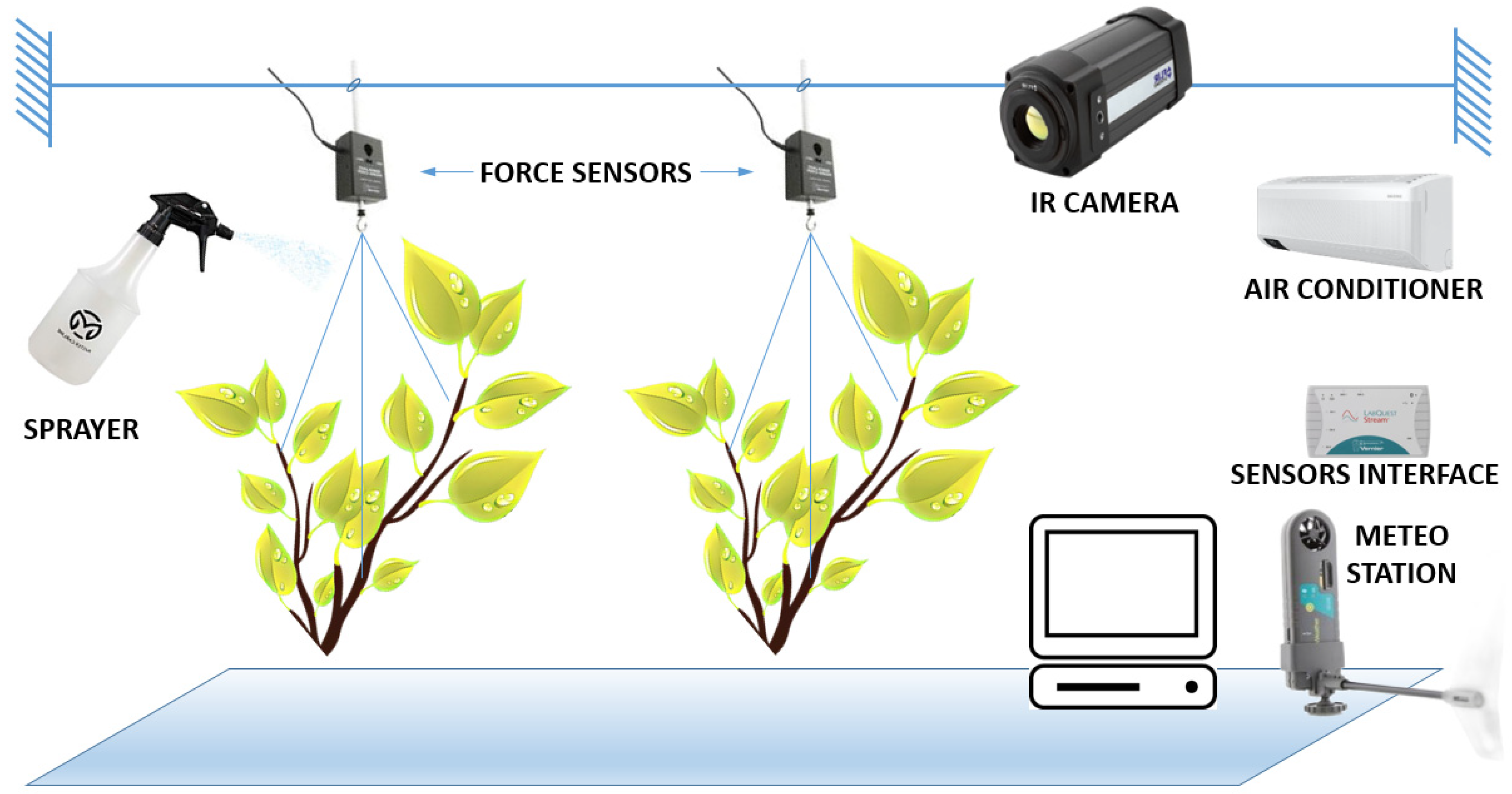
Figure 1 shows the experimental layout where for branches of lemon trees (Citrus limon (L.) Osbeck), interception capacity, S (mm) and evaporation depth E (mm), starting from S, were measured. For each run, two branches of lemon trees that were not wilting were selected from the field. After the selection, each was cut, taken immediately to the laboratory and weighted. By using a thin nylon thread (0.3 mm), for data acquisition, the dry branches were suspended on the balance arrangement by using two force sensors connected to an interface with a range of ±10 N and a sensitivity of 0.01 N, as shown in Figure 1. A weather sensor was also connected to the interface for temperature and relative humidity data acquisition. Temperature and relative humidity were imposed by using a common air conditioner, which was employed to mimic different climatic conditions. A thermal camera, FLIR A320 (IR camera), was also used to monitor the evaporation process.
Rainfall was simulated by using a common sprayer (Figure 1) until the interception capacity S was achieved. After the branches were saturated, when dripping stopped, branch weight, temperature and relative humidity data were recorded at an interval of 2 min. The slight transpiration losses, depending on the capacitance of the plant and on the evaporation process itself, were assumed as an additional evaporation loss or as negligible, according to the fact that transpiration may have been inhibited by the wet branch conditions [40,41,42,43], and also given the limited duration of the tests and the absence of solar radiation.
Tests were considered as completed when the weight of the evaporated water matched the weight corresponding to the interception capacity, thus including the water intercepted by leaves, woody parts and bark [44]. At the end of the test, the individual leaves were separated from the branches and scanned by using a Fiji image processing package [45], which made it possible to measure the number of leaves, #L, and leaf surface area, LA. The interception capacity in terms of water depth, S (mm), was calculated as the ratio between the intercepted water volume at saturation, thus including woody parts and bark, but it was referred to the leaf surface area, LA.
It is also important to note that indoor experiments were performed, so the important factors of solar radiation and wind speed were not considered. However, these issues, the effects of which are known, should be the focus of further research.
4. Results
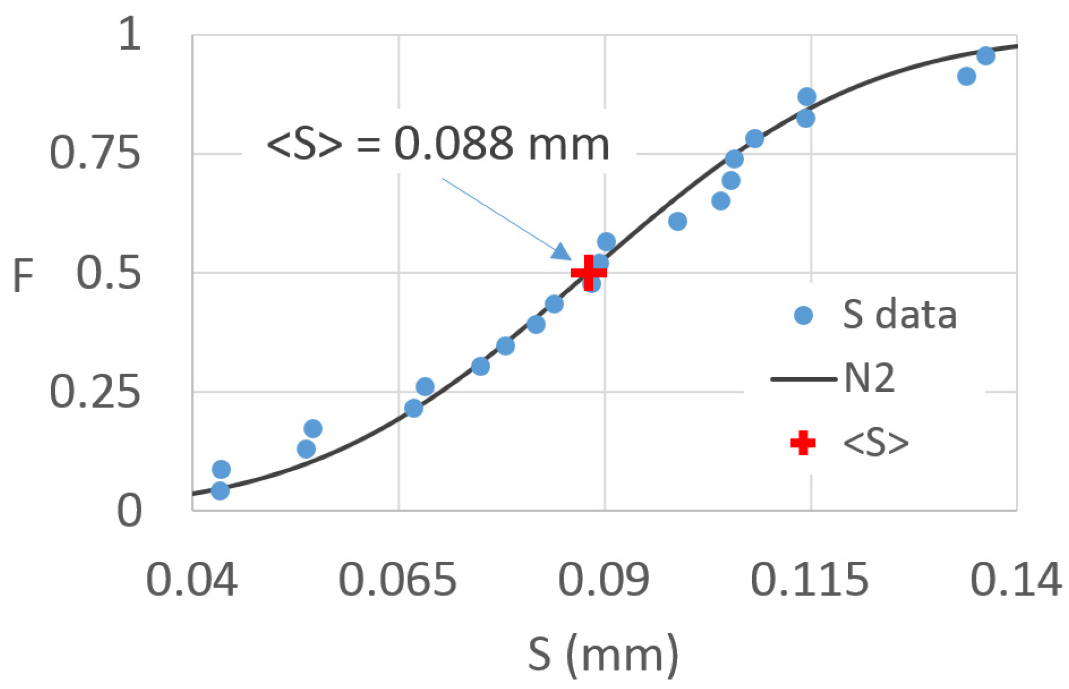
For branches of lemon trees with different numbers of leaves, #L, and leaf surface areas, LA (m2), 22 runs were carried out (Table 1), providing different values of the interception capacity, S (mm), as can be observed in Table 1. Dealing with the same tree species, a wide S variability was not expected, which contrarily occurred with a coefficient of variation CV = 30%. Figure 2 shows the frequency distribution of S that it was fitted by a normal distribution well, meaning that the average value <S> = 0.088 mm could be considered as the significant interception capacity for the investigated lemon tree branches. However, such S variability significantly affected the interpretation of the evaporation measurements, as is shown later.
The S variability was explained by many reasons, e.g., (i) the actual leaf moisture content that may determine different leaf shapes, thus affecting the maximum water amount that can be stored on the branches, and so the interception capacity; (ii) during the wetting process, not only could the upper side of the leaves be wetted, but indeed, wetting the lower side of the leaves could result in an S increase; (iii) the actual condition of the surface leaf roughness, which can change according to the presence of sand by previous rainfall events, (iv) the drop size effect [10,11]. Point (iii) is supported by the S values obtained from lemon branches sampled at the same time (denoted with the code a and b in Table 1), which provided similar values of the interception capacity.
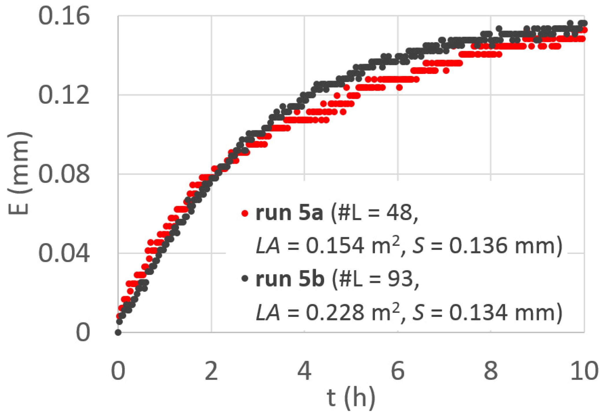
For example, Figure 3 shows the E versus the time relationship, corresponding to run 5a and 5b, thus sampled at the same time, providing very close S values (0.136 and 0.134 mm, respectively), despite the different number of leaves, #L, and leaf surface area, LA, values, as displayed in Figure 3. However, in the case of Figure 3, it can also be observed that the evaporation depth of the wet canopy exceeds the interception capacity (S). This occurrence was probably due to the transpiration effect, meaning that for run 5, the branches lost more water than that evaporated from the wet leaves.
For these runs, the E versus t relationships were also almost similar each other, indicating the suitability of the experimental data that, per unit surface areas, are independent of the size of the sampled branches. Interestingly, Table 1 shows that high tmax values are associated with runs carried out for the same branches previously tested, denoted with the code R, especially for high temperatures (1aR and 1bR, <T> = 26.6 °C). This is because when performing measurements on branches already tested, different leaf shapes occurred. However, this occurrence was not detected in run 4 and 9 at lower temperatures.
As described in the previous section, different temporal variations in the E relationships were analysed, and the semi-log relationship provided the best fitting.
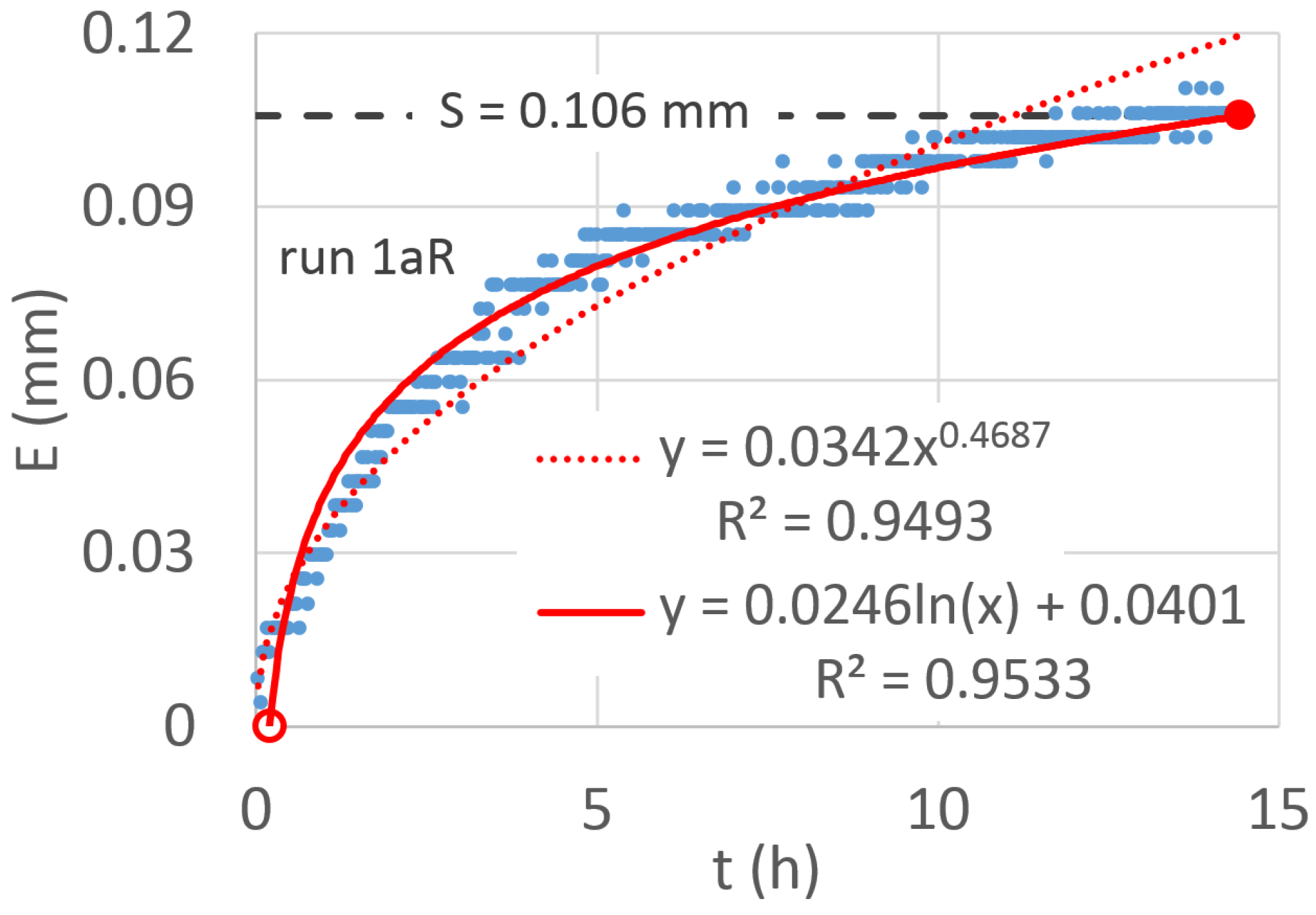
As an example, for E experimental data vs. time, obtained for run #1aR, Figure 4 shows the comparison between the fittings of the power-law (Equation (2)) considered by Baiamonte [23] and of the semi-log relationship (Equation (6)). For the latter, t0 (red circle) and tmax (red dot) and the corresponding interception capacity, S, are also indicated. Although high coefficients of determination were obtained for both cases, it can be observed that the power-law overestimated the evaporation near to the S achievement.
4.1. Parameters Estimation
Once the best fitting relationship was selected (Equation (6)), the corresponding regression coefficients n and m were estimated according to the ordinary least squares method and are reported in Table 1, together with the correlation coefficient, R, t0, tmax and the ratio E/S close to the unity, with E the measured E value at t = tmax.
Table 1 also reports the mean relative humidity, <RH>, the mean temperature, <T>, and the vapour pressure deficit, VPD, which were associated with each run. This is because, as mentioned above, different T and RH values were imposed by using an air conditioner, the thermostat of which maintained constant RH and T values, but with a certain variability around the average values. In Table 1, the corresponding coefficient of variations, CV(RH) and CV(T), are also reported. A statistical ANOVA to analyse the significance of n and m parameters was performed by choosing S, VPD and T as independent variables, which actually may have affected the evaporation measurements (Table 2, Table 3 and Table 4).
For n and m parameters, Table 2 reports the regression statistics, indicating high values of the regression coefficients with low values of the standard errors. Table 3 reports the results of ANOVA in terms of the linear multiple regression, illustrating the good performance of the selected multiple regression model, whereas in Table 4, ANOVA is referred to the considered explanatory variables.
As can be observed in Table 4, the S variable explains most of the n and m variability, especially for the n parameter, whereas the relative humidity, much more than the temperature, plays an important role in describing the m parameter.
Moreover, the signs of the coefficients of the explanatory variables agreed with their physical meaning, with the exception of the coefficient sign of T for the n parameter. RH and S were statistically significant for the m parameter, which indicated one-hour evaporation depth. Contrarily, the n parameter, i.e., the shape factor of Equation (6), as observed above, was mostly explained by the interception capacity alone. The latter agrees with the consideration that for high S values, evaporation fluxes and the drying speed quickly increase and vice versa.
The multiple linear regression (Table 4) provided the following n and m relationships:
where in Equation (12), the numerical constants, a, a1, a2 and a3, are equal to 0.0035, 0.2724, 3.07 × 10⁻³ and −3.03 × 10⁻⁴, whereas in Equation (13), the numerical constants, b, b1, b2 and b3, equal to 0.0266, 0.3334, 3.38 × 10⁻² and −1.28 × 10⁻³, respectively, and the over line symbol indicates the mean value.
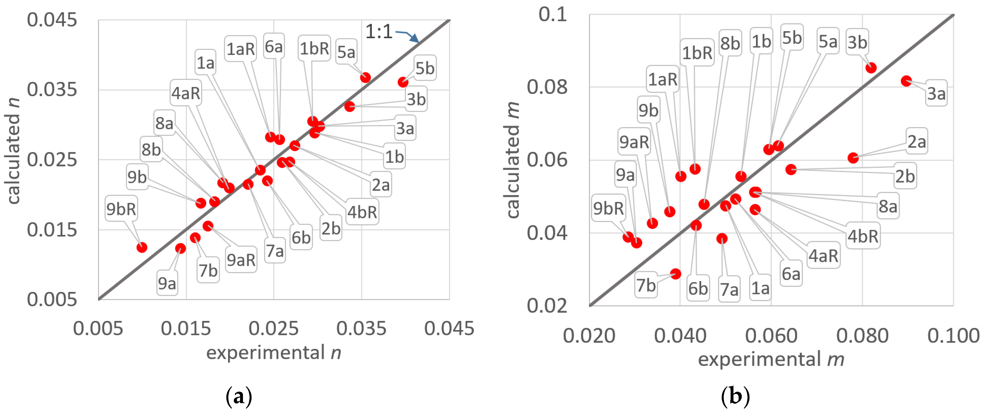
In Figure 5, n and m estimated by using the experimental data are compared with those calculated using Equation (12) and Equation (13), respectively. The figure shows that for n parameter (Figure 5a), the dots are almost close to the line of perfect agreement, indicating the good performance of Equation (12) in explaining the shape parameter of the semi-log relationship, which is linked to the evaporation rate. Meanwhile, a wider dot dispersion around the 1:1 line was obtained for the m parameter (Figure 5b).
It is interesting to observe that many of the dispersed data refer to runs carried out in branches already used to determine the E vs. t relationships (code R), indicating that the modifications of leaves’ shapes not accounted for in the selected explanatory variables could have an important role in describing the amount of water that evaporates after one hour (m parameter). Meanwhile, this effect seems to play a minor role in the evaporation rate (Figure 5a).
The consistency of the numerical constants could be better checked by analysing the influence of the physical variables on the E versus t relationships. Towards this aim, substituting Equations (12) and (13) into Equation (6), and grouping the numerical constants provide:
For any time t, the abovementioned consistence should be proved by the following conditions:
Indeed, it should be expected that with increasing S, VPD and T, evaporation should increase. In a simpler way, Equations (15)–(17) could be applied for fixed VPD, by varying T, and for fixed T, by varying VPD, to check their expected influence on E.
For a fixed S equal to the mean value (S = 0.088 mm) and for T = 25 °C, Figure 6a shows E versus t, for different VPDs (VPD = 1, 1.5 and 2 kPa, Figure 6a), whereas in Figure 6b, for VPD = 1.5 kPa, E versus t is plotted for different Ts (T = 20, 24 and 28 °C). The figure shows that for both VPD and T, the expected trends occur, indicating the suitability of the calibrated model, and thus the influence on the evaporation process by the considered physical variables. However, it seems that VPD has greater importance than T, also supported by the ANOVA, at least in the considered range of the investigated variables.
From a practical point of view, the usefulness of such calibrated relationships lays in their ability to estimate the evaporation losses, starting with any initial conditions, t0, when applied in combination with an interception model, such as that suggested by Baiamonte [23].
A more extended validation of such a procedure was performed by considering that the evaporation losses are only described by the shape parameter, n, of the semi-log relationship, as observed in the previous section:
where DS (h) is the dry spell duration for which the evaporation loss has to be estimated.
With this aim, the experimental data and those corresponding to the fitting relationships were disaggregated to check the procedure for many possible combinations of the pairs (E0, E) and (t0, t). Thus, for each run, r, the combinations Nr = n (n −1)/2! of disaggregated data were considered, with n equal to the number of the sampled E values for each run.
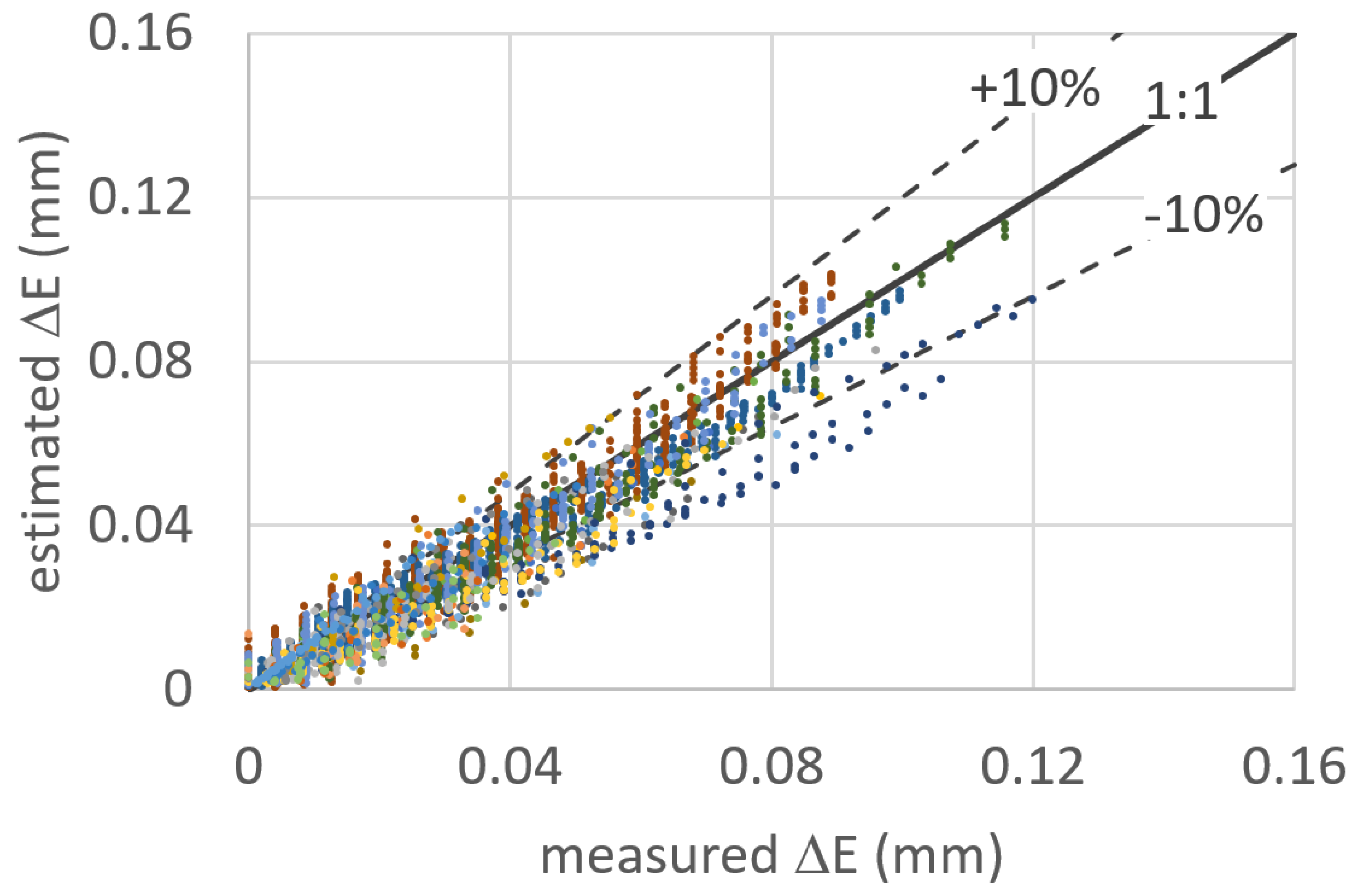
Because of the high number, n, of the experimental E values, N22 = Σ Nr = 2812 disaggregated data were obtained and compared with the data calculated using Equation (18). The results of the comparison are reported in Figure 7, where the line of perfect agreement is also indicated. The standard error of the estimate, SEE, of ΔE was equal to 0.007 mm, which is not much if considering the complexity of the studied process. In the same Figure 7, two straight lines bounding the domain corresponding to a maximum estimate error equal to ±10% are plotted. Excluding the minor number of cases, the points fall inside of this field, proving the reliability of the suggested procedure.
4.2. Using IR Images
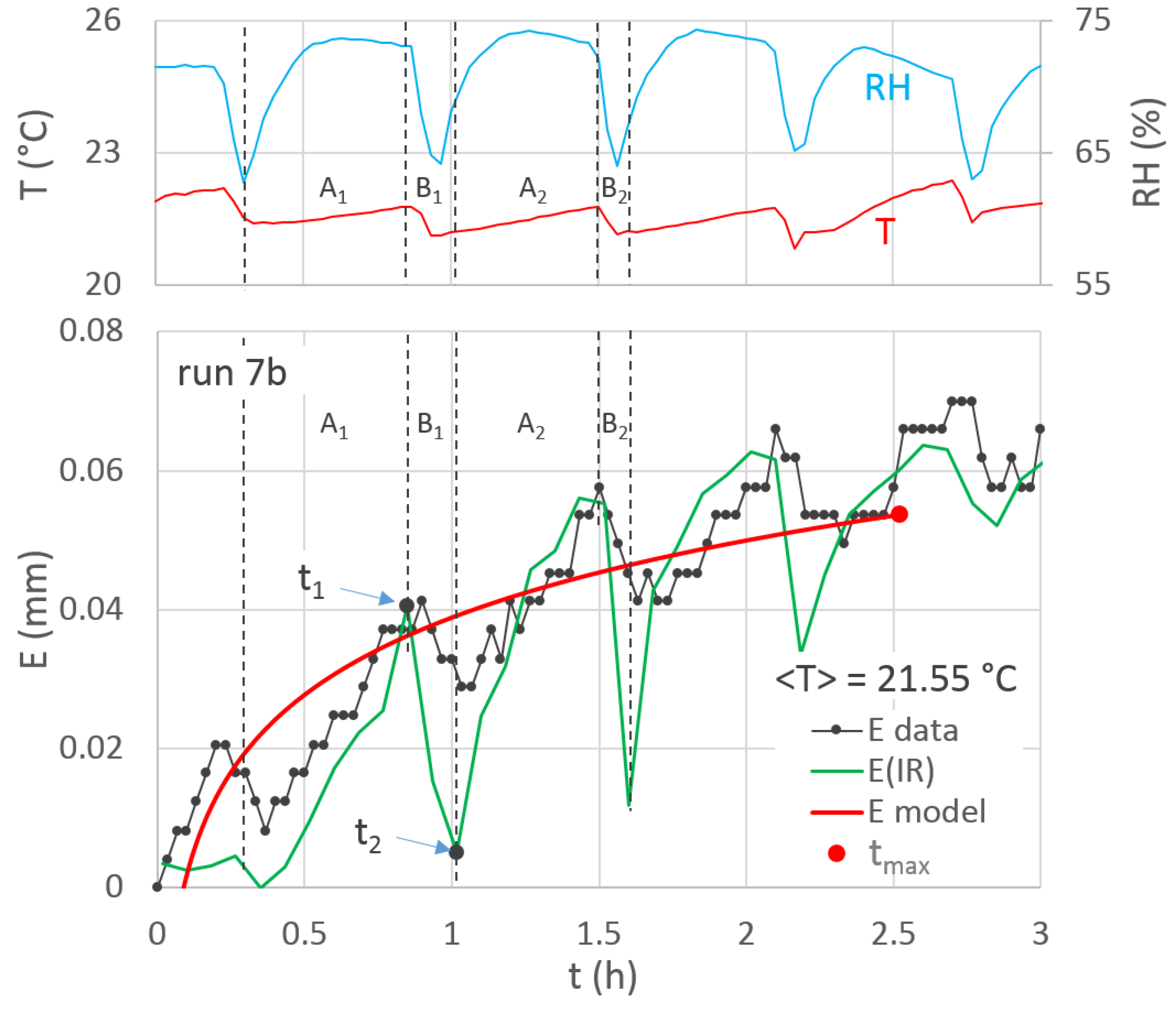
For the runs carried out with low values of the mean temperature (such as #4aR, #4bR, #7a and #7b), the non-monotonic behaviour of the E temporal variation was observed. As an example, for run 7b, for which a slight T variability occurred (<T> = 21.6 °C), Figure 8 shows that the experimental E values started increasing and then decreasing versus the time, mostly because of the RH and VPD variations that were determined by the air conditioner, which maintained the temperature using a temperature sensor associated with a controller. It is known that the sensor read the return air temperature from the room which was air-conditioned and the controller compared it with the set point. Once the set point was achieved the controller, cut down the compressor which in turn stopped the room being cooled more, and so on.
While the intermittent compressor functioning did not provide significant effects for high temperatures, for low temperatures, the RH (and VPD) role on E became more and more evident at decreasing T. The E decreasing steps were clearly due to a condensing process so that the leaves were enriched by the water vapour in air that condensed on the cool leaves.
This was more due to RH (and VPD) than to T variation, with the latter exhibiting smaller variations than RH (Figure 8). As can be observed by the domains A1, A2, B1 and B2 displayed in Figure 8, a certain condensation delay with respect to the RH increasing occurred, so if in the range A1, RH increased, its effect in terms of condensation (E decreasing) occurred in the subsequent range B1, and so for A2 and B2. This is probably due to the fact that inertial effects occurred after the RH reading increased, which causes the vapour condensation with some delay.
As can be observed in Figure 8, for these cases as well, the semi-log relationship was considered, providing an average behaviour of the non-monotonic E relationship. This issue, which was of course determined by the selected experimental set up, complicated the interpretation of the experimental data and contributed to explaining the aforementioned errors associated with E estimation by means of VPD, T and S data.
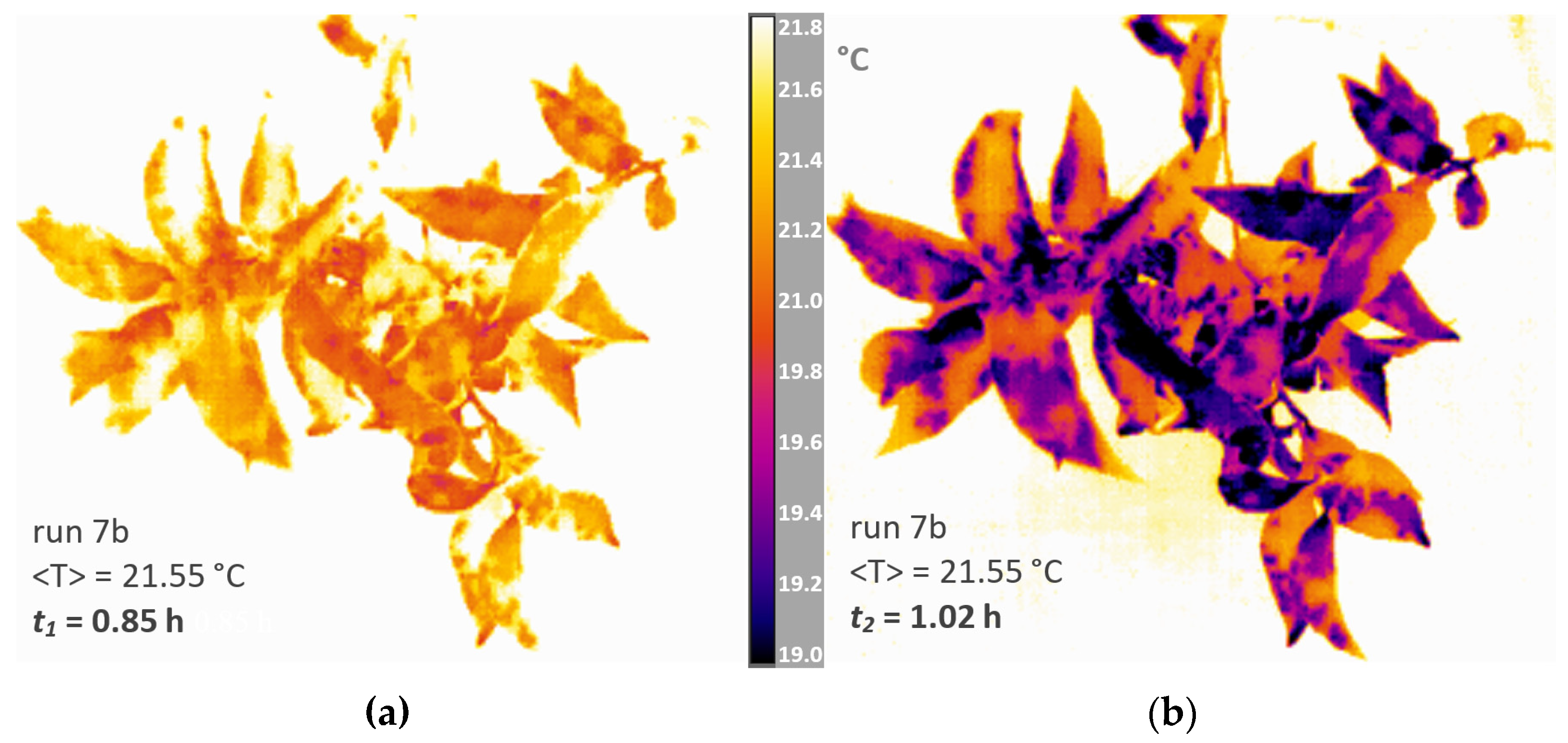
A deeper analysis was performed for the 7b run by using the IR camera (Figure 1) recording infrared images during the evaporation process. Since the leaf surface temperature changed according to the amount of water stored on the branches, it was assumed that the number of pixels corresponding to a range of temperatures denoted the evaporation for any fixed time t. In particular, the evaporation losses derived by the IR images, E(IR), were rescaled according to:
where S is the interception capacity for run 7b (Table 1), Tmax is the temperature for dry conditions (21.8 °C), Nt is the number of pixels at the time t, for which T < Tmax, and Nmax is the total number of pixels of the sampled branch. Of course, when the run starts, Nt = Nmax and E(IR) = 0, whereas for dry conditions (Nt = 0), E(IR) = S. The E(IR) values derived in such way are plotted in Figure 8, showing similar behaviour to E data obtained by the force sensors, thus confirming the alternation of the condensation and of the evaporation processes provided by the direct measurements.
The overestimated condensation obtained using IR images (Figure 8, B1 and B2) could be ascribed to the heat transfer from the leaves to the water stored on the branches that determines a leaf cooling down, which should be carefully considered when upscaling such procedure.
Two IR images corresponding to the times t1 and t2, for which highly different E values occurred, are plotted in Figure 9, where the same T scale at t1 = 0.85 h (Figure 9a) and, after 10 min, at t2 = 1.02 h (Figure 9b) was set. The latter made it possible to observe the condensation process during step B1 (Figure 8), thus validating the E versus t relationship obtained by the force sensors under T and RH conditions.
5. Conclusions
In a recent work, a simplified interception/evaporation model was proposed [23], which considers a modified Merrian model to compute interception during wet spells and a simple power-law equation to model evaporation from a wet canopy during dry spells. The modelling evaporation process at the sub hourly temporal scale required the two parameters of the power-law, describing the hourly evaporation depth and the evaporation rate.
In this paper, we focused on the evaporation process from wet branches of lemon trees starting from the interception capacity, S. For different temperature, T, and vapour pressure deficit, VPD, conditions, numerous experimental tests were carried out. In addition to the abovementioned power-law, simple models were applied and tested, and the semi-log model provided the best fitting to the evaporation data. Two parameters, physically linked to the evaporation fluxes and to the evaporation amount from the wet branches, were determined and correlated to T, S, and to vapour pressure deficit, VPD.
We are aware that the experimental measurements carried out in the laboratory were affected by various uncertainties and approximations, such as a lack of consideration for solar radiation, resulting in sensible heat flux in the air. Moreover, we are aware that the model based on indoor experiments, thus neglecting wind speed, did not follow a rigorous procedure to enable it to be applicable under field conditions and for crops that differ from lemon trees. However, the results obtained in this work help us to understand the studied process, highlight its complexity and could be implemented in the recently introduced interception/evaporation model to quantify, under the abovementioned limitations, this important component of the hydrologic cycle.
Author Contributions
Conceptualization, G.B.; methodology, G.B.; formal analysis, G.B.; investigation, G.B. and S.P.; resources, G.B.; data curation, G.B. and S.P.; writing—original draft preparation, G.B. and S.P.; writing—review and editing, G.B. and S.P.; visualization, G.B.; supervision, G.B. All authors have read and agreed to the published version of the manuscript.
Funding
This research received no external funding.
Data Availability Statement
The data presented in this study are available on request from the corresponding author.
Acknowledgments
The authors wish to thank the anonymous reviewers for their helpful comments and their careful reading of the manuscript during the revision stage.
Conflicts of Interest
The authors declare no conflict of interest.
References
- Gerrits, A.M.J.; Savenije, H.H.G. Treatise on Water Science; Wilderer, P., Ed.; Elsevier: Amsterdam, The Netherlands, 2010. [Google Scholar]
- Baiamonte, G. Simplified model to predict runoff generation time for well-drained and vegetated soils. J. Irrig. Drain. Eng. 2016, 142, 04016047. [Google Scholar] [CrossRef]
- Uddin, J.; Foley, J.P.; Smith, R.J.; Hancock, N.H. A new approach to estimate canopy evaporation and canopy interception capacity from evapotranspiration and sap flow measurements during and following wetting. Hydrol. Process. 2015, 30, 1757–1767. [Google Scholar] [CrossRef]
- Savenije, H.H.G. The importance of interception and why we should delete the term evapotranspiration from our vocabulary. Hydrol. Process. 2004, 18, 1507–1511. [Google Scholar] [CrossRef]
- Beven, K.J. Rainfall–Runoff Modelling: The Primer; John Wiley & Sons: Chichester, UK, 2001; ISBN 0-471-98553-8. [Google Scholar]
- Calder, I.R. Evaporation in the Uplands; John Wiley & Sons: Chichester, UK, 1990; ISBN 0-471-92487-3. [Google Scholar]
- Carlyle-Moses, D.E. Throughfall, stemflow, and canopy interception loss fluxes in a semi-arid Sierra Madre Oriental matorral community. J. Arid Environ. 2004, 58, 181–202. [Google Scholar] [CrossRef]
- Wu, J.; Liu, L.; Sun, C.; Su, Y.; Wang, C.; Yang, J.; Liao, J.; He, X.; Li, Q.; Zhang, C.; et al. Estimating Rainfall Interception of Vegetation Canopy from MODIS Imageries in Southern China. Remote Sens. 2019, 11, 2468. [Google Scholar] [CrossRef] [Green Version]
- Bagarello, V.; Baiamonte, G.; Caia, C. Variability of near-surface saturated hydraulic conductivity for the clay soils of a small Sicilian basin. Geoderma 2019, 340, 133–145. [Google Scholar] [CrossRef]
- Calder, I.R. Canopy processes: Implications for transpiration, interception and splash induced erosion, ultimately for forest management and water resources. Plant. Ecol. 2001, 153, 203–214. [Google Scholar] [CrossRef]
- Hall, R.L.; Calder, I.R. Drop Size Modification by Forest Canopies’ Measurements Using a Disdrometer. J. Geophys. 1993, 98, 18465–18470. [Google Scholar] [CrossRef]
- Page, T.; Chappell, N.A.; Beven, K.; Hankin, B.; Kretzschmar, A. Assessing the significance of wet-canopy evaporation from forests during extreme rainfall events for flood mitigation in mountainous regions of the United Kingdom. Hydrol. Process. 2020, 34, 4740–4754. [Google Scholar] [CrossRef]
- Jiao, J.; Su, D.; Han, L.; Wang, Y. A Rainfall Interception Model for Alfalfa Canopy under Simulated Sprinkler Irrigation. Water 2016, 8, 585. [Google Scholar] [CrossRef] [Green Version]
- Muzylo, A.; Llorens, P.; Valente, F.; Keizer, J.J.; Domingo, F.; Gash, J.H.C. A review of rainfall interception modelling. J. Hydrol. 2009, 370, 191–206. [Google Scholar] [CrossRef] [Green Version]
- Rutter, A.J.; Kershaw, K.A.; Robins, P.C.; Morton, A.J. A predictive model of rainfall interception in forests, 1. Derivation of the model from observations in a plantation of Corsican pine. Agric. Meteorol. 1971, 9, 367–384. [Google Scholar] [CrossRef]
- Rutter, A.J.; Morton, A.J.; Robins, P.C. A predictive model of rainfall interception in forests. II. Generalization of the model and comparison with observations in some coniferous and hardwood stands. J. Appl. Ecol. 1975, 12, 367–380. [Google Scholar] [CrossRef]
- Calder, I. A model of transpiration and interception loss from a spruce forest in Plynlimon, Central Wales. J. Hydrol. 1977, 33, 247–265. [Google Scholar] [CrossRef]
- Gash, J.; Morton, A. Application of the Rutter model to the estimation of the interception loss from Thetford forest. J. Hydrol. 1978, 38, 49–58. [Google Scholar] [CrossRef]
- Linsley, R.K., Jr.; Kohler, M.A.; Paulhus, J.L. Applied Hydrology; McGraw-Hill Book Co.: New York, NY, USA, 1988. [Google Scholar]
- Horton, R.E. Rainfall interception. Mon. Weather Rev. 1919, 47, 603–623. [Google Scholar] [CrossRef]
- Merriam, R.A. A note on the interception loss equation. J. Geophys. Res. 1960, 5, 3850–3851. [Google Scholar] [CrossRef]
- Merriam, R.A. Fog drip from artificial leaves in a fog wind tunnel. Water Resour. Res. 1973, 9, 1591–1598. [Google Scholar] [CrossRef]
- Baiamonte, G. Simplified Interception/Evaporation Model. Hydrology 2021, 8, 99. [Google Scholar] [CrossRef]
- Babu, A.K.; Kumaresan, G.; Raj, V.A.A.; Velraj, R. Review of leaf drying: Mechanism and influencing parameters, drying methods, nutrient preservation, and mathematical models. Renew. Sustain. Energy Rev. 2018, 90, 536–556. [Google Scholar] [CrossRef]
- Pumo, D. L’Approvvigionamento Idrico per l’Agricoltura; Aracne Editrice SRL: Rome, Italy, 2008; ISBN 978-88-548-1708-1. (In Italy) [Google Scholar]
- Crockford, R.H.; Richardson, D.P. Partitioning of rainfall into throughfall, stemflow and interception: Effect of forest type, ground cover and climate. Hydrol. Process. 2000, 14, 2903–2920. [Google Scholar] [CrossRef]
- Garcia-Estringana, P.; Alonso-Blázquez, N.; Alegre, J. Water storage capacity, stemflow and water funneling in Mediterranean shrubs. J. Hydrol. 2010, 389, 363–372. [Google Scholar] [CrossRef]
- Hancock, N.H.; Crowther, J.M. A technique for the direct measurement of water storage on a forest canopy. J. Hydrol. 1979, 41, 105–122. [Google Scholar] [CrossRef]
- Huang, Y.S.; Chena, S.S.; Lin, T.P. Continuous monitoring of water loading of trees and canopy rainfall interception using the strain gauge method. J. Hydrol. 2005, 311, 1–7. [Google Scholar] [CrossRef]
- Aston, A.R. Rainfall interception by eight small trees. J. Hydrol. 1979, 42, 383–396. [Google Scholar] [CrossRef]
- Liu, S. Estimation of rainfall storage capacity in the canopies of cypress wetlands and slash pine uplands in North-Central Florida. J. Hydrol. 1998, 207, 32–41. [Google Scholar] [CrossRef]
- Gash, J.H.C.; Lloyd, C.R.; Lachaudb, G. Estimating sparse forest rainfall interception with an analytical model. J. Hydrol. 1995, 170, 79–86. [Google Scholar] [CrossRef]
- Sadeghi, S.M.M.; Attarod, P.; Grant Pypker, T.; Dunkerley, D. Is canopy interception increased in semiarid tree plantations? Evidence from a field investigation in Tehran, Iran. Turk. J. Agric. For. 2015, 38, 792–806. [Google Scholar] [CrossRef]
- Zhang, Q.; Lv, X.; Yu, X.; Ni, Y.; Ma, L.; Liu, Z. Species and spatial differences in vegetation rainfall interception capacity: A synthesis and meta-analysis in China. Catena 2022, 213, 106223. [Google Scholar] [CrossRef]
- Helvey, J.D.; Patric, J.H. Canopy and Litter Interception of Rainfall by Hardwoods of Eastern United States. Water Resour. Res. 1965, 1, 193–206. [Google Scholar] [CrossRef] [Green Version]
- Eliades, M.; Bruggeman, A.; Djuma, H.; Christou, A.; Rovanias, K.; Lubczynski, M.W. Testing three rainfall interception models and different parameterization methods with data from an open Mediterranean pine forest. Agric. For. Meteorol. 2022, 313, 108755. [Google Scholar] [CrossRef]
- Black, T.A.; Gardner, W.R.; Thurtell, G.W. The prediction of evaporation, drainage, and soil water storage for a bare soil. Soil Sci. Soc. Amer. Proc. 1969, 33, 655–660. [Google Scholar] [CrossRef]
- Ritchie, J.T. Model for predicting evaporation from a row crop with incomplete cover. Water Resour. Res. 1972, 8, 1204–1213. [Google Scholar] [CrossRef] [Green Version]
- Baiamonte, G. Dimensionless Stage-Discharge Relationship for a Non-Linear Water Reservoir: Theory and Experiments. Hydrology 2020, 7, 23. [Google Scholar] [CrossRef] [Green Version]
- Medrado, J.P.T.; Inman, R.H.; Coimbra, C.F.M. Isothermal and near-isothermal free evaporation of water from open tubes in air. Int. J. Heat Mass Transf. 2022, 189, 122687. [Google Scholar] [CrossRef]
- Alvarado-Barrientos, M.S.; Holwerdab, F.; Asbjornsena, H.; Dawsonc, T.E.; Bruijnzeel, L.A. Suppression of transpiration due to cloud immersion in a seasonally dry Mexican weeping pine plantation. Agric. For. Meteorol. 2014, 186, 12–25. [Google Scholar] [CrossRef]
- Aparecido, L.M.T.; Miller, G.R.; Cahill, A.T.; Moore, G.W. Comparison of tree transpiration under wet and dry canopy conditions in a Costa Rican premontane tropical forest. Hydrol. Process. 2016, 30, 5000–5011. [Google Scholar] [CrossRef]
- Baiamonte, G.; Motisi, A. Analytical approach extending the Granier method to radial sap flow patterns. Agric. Water Manage. 2020, 231, 105998. [Google Scholar] [CrossRef]
- Iida, S.; Levia, D.F.; Shimizu, A.; Shimizu, T.; Tamai, K.; Nobuhiro, T.; Kabeya, N.; Noguchi, S.; Sawano, S.; Araki, M. Intrastorm scale rainfall interception dynamics in a mature coniferous forest stand. J. Hydrol. 2017, 548, 770–783. [Google Scholar] [CrossRef]
- Schindelin, J.; Arganda-Carreras, I.; Frise, E.; Cardona, A. Fiji: An open-source platform for biological-image analysis. Nat. Methods 2012, 9, 676–682. [Google Scholar] [CrossRef] [Green Version]
Figure 1.
Sketch of the experimental layout.

Figure 2.
For the considered 22 runs, frequency distribution and normal distribution, N2, of the interception capacity, S. The mean value <S> is also indicated.
Figure 2.
For the considered 22 runs, frequency distribution and normal distribution, N2, of the interception capacity, S. The mean value <S> is also indicated.

Figure 3.
For runs #5a and #5b, temporal variation of the evaporation depth by the wet branches.

Figure 4.
For runs #1aR, temporal variation of the evaporation depth and the corresponding fitted power-law and semi-log relationship. The t0 (red circle) and tmax (red dot) values are also indicated.
Figure 4.
For runs #1aR, temporal variation of the evaporation depth and the corresponding fitted power-law and semi-log relationship. The t0 (red circle) and tmax (red dot) values are also indicated.

Figure 5.
For the 22 runs, comparison between the parameters obtained using the ordinary least squares method applied to the experimental pairs (E,t) and those calculated (a) using Equation (12) for the n parameter and (b) using Equation (13) for the m parameter.
Figure 5.
For the 22 runs, comparison between the parameters obtained using the ordinary least squares method applied to the experimental pairs (E,t) and those calculated (a) using Equation (12) for the n parameter and (b) using Equation (13) for the m parameter.

Figure 6.
Performance of the simplified evaporation model (a) for fixed temperature T, by varying the vapour pressure deficit, VPD, and (b), for fixed VPD, by varying the temperature, T.
Figure 6.
Performance of the simplified evaporation model (a) for fixed temperature T, by varying the vapour pressure deficit, VPD, and (b), for fixed VPD, by varying the temperature, T.

Figure 7.
For the 22 runs, comparison between the evaporation loss, ΔE, obtained for multiple combinations of the time interval, Δt, with those calculated using Equation (18). The two straight lines bound the domain corresponding to a maximum estimate error equal to ±10%.
Figure 7.
For the 22 runs, comparison between the evaporation loss, ΔE, obtained for multiple combinations of the time interval, Δt, with those calculated using Equation (18). The two straight lines bound the domain corresponding to a maximum estimate error equal to ±10%.

Figure 8.
For run 7b, comparison between the temporal variation of the evaporation depth obtained by the experimental data with that obtained by the semi-log relationship (Equation (6)), and with that determined using IR images, E(IR), Equation (19). The time t1 and t2, corresponding to Figure 9, for which water condensation occurred on the leaves, are indicated.

Figure 9.
For run 7b, corresponding to Figure 7a, thermal images recorded (a) at the time t1 = 0.85 h and (b) at the time t2 = 1.02 h.
Figure 9.
For run 7b, corresponding to Figure 7a, thermal images recorded (a) at the time t1 = 0.85 h and (b) at the time t2 = 1.02 h.


Table 1.
For the 22 runs, number of leaves, #L, leaf area, LA, interception capacity, S, mean relative humidity and temperature, <RH> and <T>, with the corresponding coefficient of variation, CV, vapour pressure deficit, VPD, n and m parameters, correlation coefficient, characteristic times, t0 and tmax, and the ratio E/S.
| run # | #L | LA (m2) | S (mm) | <RH> (%) | CV(RH) | <T> (°C) | CV(T) | VPD | n | m | R | t0 (h) | tmax (h) | E/S |
|---|---|---|---|---|---|---|---|---|---|---|---|---|---|---|
| 1a | 34 | 0.149 | 0.089 | 64.9 | 1.1% | 26.5 | 0.8% | 1.212 | 0.0234 | 0.0499 | 0.905 | 0.119 | 5.38 | 1.00 |
| 1b | 140 | 0.293 | 0.108 | 63.6 | 3.1% | 26.7 | 1.4% | 1.276 | 0.0296 | 0.0533 | 0.935 | 0.165 | 6.39 | 1.02 |
| 1aR | 34 | 0.149 | 0.106 | 62.8 | 3.0% | 26.6 | 1.2% | 1.294 | 0.0246 | 0.0401 | 0.976 | 0.196 | 14.44 | 1.00 |
| 1bR | 140 | 0.293 | 0.114 | 63.5 | 2.4% | 26.7 | 1.2% | 1.274 | 0.0294 | 0.0432 | 0.979 | 0.230 | 11.29 | 0.98 |
| 2a | 76 | 0.148 | 0.099 | 56.2 | 1.8% | 26.3 | 1.3% | 1.498 | 0.0274 | 0.0779 | 0.976 | 0.058 | 2.15 | 1.00 |
| 2b | 48 | 0.162 | 0.090 | 56.5 | 1.9% | 26.3 | 1.1% | 1.486 | 0.0259 | 0.0642 | 0.975 | 0.084 | 2.72 | 1.05 |
| 3a | 52 | 0.153 | 0.104 | 45.9 | 1.7% | 29.7 | 0.5% | 2.260 | 0.0302 | 0.0896 | 0.983 | 0.051 | 1.61 | 1.04 |
| 3b | 93 | 0.205 | 0.114 | 46.0 | 1.6% | 29.9 | 1.0% | 2.275 | 0.0336 | 0.0819 | 0.979 | 0.088 | 2.63 | 1.06 |
| 4aR | 38 | 0.162 | 0.075 | 58.8 | 6.4% | 18.5 | 1.6% | 0.877 | 0.0199 | 0.0563 | 0.957 | 0.059 | 2.55 | 1.10 |
| 4bR | 62 | 0.157 | 0.088 | 58.4 | 6.6% | 18.5 | 1.7% | 0.888 | 0.0268 | 0.0562 | 0.963 | 0.122 | 3.33 | 0.96 |
| 5a | 48 | 0.154 | 0.136 | 63.1 | 1.5% | 23.8 | 1.0% | 1.088 | 0.0354 | 0.0615 | 0.970 | 0.176 | 8.26 | 1.06 |
| 5b | 93 | 0.228 | 0.134 | 63.4 | 1.3% | 23.8 | 1.0% | 1.081 | 0.0397 | 0.0594 | 0.954 | 0.224 | 6.52 | 1.06 |
| 6a | 33 | 0.145 | 0.105 | 67.5 | 1.3% | 24.1 | 0.9% | 0.977 | 0.0256 | 0.0522 | 0.977 | 0.131 | 7.97 | 1.00 |
| 6b | 68 | 0.228 | 0.084 | 67.6 | 1.4% | 24.2 | 0.9% | 0.976 | 0.0242 | 0.0434 | 0.954 | 0.167 | 5.29 | 1.07 |
| 7a | 63 | 0.186 | 0.082 | 70.8 | 4.2% | 21.6 | 1.4% | 0.751 | 0.0220 | 0.0491 | 0.957 | 0.108 | 4.37 | 1.13 |
| 7b | 64 | 0.154 | 0.054 | 71.4 | 4.1% | 21.6 | 1.3% | 0.736 | 0.0160 | 0.0389 | 0.899 | 0.088 | 2.52 | 1.23 |
| 8a | 90 | 0.195 | 0.078 | 55.1 | 1.6% | 21.8 | 1.4% | 1.175 | 0.0191 | 0.0566 | 0.980 | 0.052 | 3.05 | 1.05 |
| 8b | 72 | 0.223 | 0.068 | 55.1 | 1.5% | 21.9 | 1.3% | 1.177 | 0.0182 | 0.0452 | 0.966 | 0.083 | 3.53 | 1.09 |
| 9a | 54 | 0.163 | 0.043 | 57.0 | 1.3% | 19.9 | 1.2% | 1.002 | 0.0144 | 0.0304 | 0.957 | 0.121 | 2.45 | 1.17 |
| 9b | 8 | 0.040 | 0.067 | 56.2 | 3.0% | 20.0 | 1.3% | 1.025 | 0.0167 | 0.0377 | 0.966 | 0.104 | 5.73 | 0.95 |
| 9aR | 54 | 0.163 | 0.055 | 55.1 | 1.3% | 20.1 | 1.1% | 1.058 | 0.0175 | 0.0338 | 0.936 | 0.144 | 3.28 | 1.07 |
| 9bR | 8 | 0.040 | 0.043 | 55.1 | 1.3% | 20.1 | 1.1% | 1.058 | 0.0099 | 0.0285 | 0.993 | 0.057 | 4.46 | 0.94 |
Table 2.
Regression statistics for n and m parameters of Equation (6).
| Regression Statistics | n | m |
|---|---|---|
| Multiple R | 0.9638 | 0.8414 |
| R Square | 0.9290 | 0.7079 |
| Adjusted R Square | 0.9172 | 0.6592 |
| Standard Error | 0.0021 | 0.0094 |
| Observations | 22 | 22 |
Table 3.
For n and m parameters, ANOVA of the linear multiple regression.
| ANOVA | df | SS | MS | F | Significance F |
|---|---|---|---|---|---|
| n parameter | |||||
| Regression | 3 | 0.0010 | 0.0003 | 78.50 | 1.56 × 10⁻¹⁰ |
| Residual | 18 | 0.0001 | 4.43 × 10⁻⁶ | ||
| Total | 21 | 0.0011 | |||
| m parameter | |||||
| Regression | 3 | 0.0038 | 0.0013 | 14.54 | 4.68 × 10⁻⁵ |
| Residual | 18 | 0.0016 | 0.0001 | ||
| Total | 21 | 0.0054 | |||
Table 4.
For n and m parameters, ANOVA of the explanatory variables.
| Explanatory Variables | Coefficients | Standard Error | t Stat | p-Value | Lower 95% | Upper 95% |
|---|---|---|---|---|---|---|
| n parameter | ||||||
| Intercept | 0.0035 | 0.0039 | 0.8960 | 0.3821 | −0.0048 | 0.0118 |
| <T> | −3.032 × 10⁻⁴ | 0.0003 | −1.0750 | 0.2966 | −0.0009 | 0.0003 |
| VPD | 3.075 × 10⁻³ | 0.0020 | 1.5376 | 0.1415 | −0.0011 | 0.0073 |
| S | 0.2724 | 0.0238 | 11.436 | 1.1×10⁻⁹ | 0.2224 | 0.3225 |
| m parameter | ||||||
| Intercept | 0.0266 | 0.0175 | 1.5168 | 0.1467 | −0.0103 | 0.0635 |
| <T> | −1.885 × 10⁻³ | 0.0013 | −1.5026 | 0.1503 | −0.0045 | 0.0008 |
| VPD | 3.386 × 10⁻² | 0.0089 | 3.8069 | 0.0013 | 0.0152 | 0.0525 |
| S | 0.3334 | 0.1060 | 3.1469 | 0.0056 | 0.1108 | 0.5560 |
Publisher’s Note: MDPI stays neutral with regard to jurisdictional claims in published maps and institutional affiliations. |
© 2022 by the authors. Licensee MDPI, Basel, Switzerland. This article is an open access article distributed under the terms and conditions of the Creative Commons Attribution (CC BY) license (https://creativecommons.org/licenses/by/4.0/).
Share and Cite
MDPI and ACS Style
Baiamonte, G.; Palermo, S. Measuring and Modelling Evaporation Losses from Wet Branches of Lemon Trees. Hydrology 2022, 9, 118. https://0-doi-org.brum.beds.ac.uk/10.3390/hydrology9070118
AMA Style
Baiamonte G, Palermo S. Measuring and Modelling Evaporation Losses from Wet Branches of Lemon Trees. Hydrology. 2022; 9(7):118. https://0-doi-org.brum.beds.ac.uk/10.3390/hydrology9070118
Chicago/Turabian StyleBaiamonte, Giorgio, and Samuel Palermo. 2022. "Measuring and Modelling Evaporation Losses from Wet Branches of Lemon Trees" Hydrology 9, no. 7: 118. https://0-doi-org.brum.beds.ac.uk/10.3390/hydrology9070118
Note that from the first issue of 2016, this journal uses article numbers instead of page numbers. See further details here.