Article

Investigation and Source Apportionment of Air Pollutants in a Large Oceangoing Ship during Voyage

Center of Disease Control and Prevention of Chinese People’s Liberation Army, Beijing 100071, China
*
Author to whom correspondence should be addressed.
Int. J. Environ. Res. Public Health 2019, 16(3), 389; https://0-doi-org.brum.beds.ac.uk/10.3390/ijerph16030389
Submission received: 10 December 2018 / Revised: 16 January 2019 / Accepted: 26 January 2019 / Published: 30 January 2019
(This article belongs to the Special Issue Transportation-Related Air Pollution and Human Health)

Abstract

:
The aims of this study were to determine compartmental air pollution during navigation of a large oceangoing ship and to identify preliminarily the major pollution sources. During the voyage of a bulk carrier ship, air samples were collected at 18 selected sites using a stratified sampling method. The concentrations of 15 pollutants were determined using gas chromatography. Results showed the concentrations of these pollutants varied significantly among the sampling sites, indicating major pollution sources at or nearby those locations. Five common factors extracted using factor analysis explained 89.092% of the total variance. Multivariate linear regression analysis showed the contributions to air pollution of these five common factors, i.e., the volatilization of ship paint, volatilization of ship-based oil, cooking activities, high-temperature release of rubber components on the ship and daily use of chemical products, and the application of deodorant and insecticide, were 41.07%, 25.14%, 14.37%, 11.78%, and 7.63%, respectively. Three significant groups were determined using cluster analysis based on their similarity, i.e., high, medium, and low pollution of sampling sites. This study established that the air of the bulk carrier ship was heavily polluted, and that effective identification of pollution sources could provide a scientific basis for its control.

Graphical Abstract

1. Introduction

Increasingly, modern oceangoing ships are constructed as closed vessels, which is a design that could result in poor natural ventilation of the indoor environment. Large oceangoing ships are generally equipped with air purification equipment; however, the confined compartments of activity of the crew, complicated pollution sources, and air recycling inevitably produce internal air pollution [1,2]. Previous studies have found that numerous organic pollutants, such as those released by diesel, gasoline, paint, and crew activities, can affect air quality during voyages of large oceangoing ships [3,4,5]. Additionally, the widespread use of nonmetallic materials in ships, e.g., plastics, fiberglass, adhesives, refrigerants, and fire extinguishers can also lead to the release of pollutants [6]. The emission of inorganic and volatile organic compounds from nonmetallic materials is one of the main sources of air pollution in ship compartments [7]. Because of extended voyage durations of large oceangoing ships, air pollutant concentrations within ship compartments are likely to increase [8]. More importantly, because of the long periods spent at sea working and living in confined compartments, the internal environment of a ship has a direct impact on the physical/mental health and work efficiency of its crew [9].
For effective pollution control and air quality management, it is necessary to identify the pollution sources and their quantitative contributions. The application of different multivariate statistical techniques can offer better understanding of indoor air quality. Principal component analysis/factor analysis can be used for qualitative determination of latent sources but not for direct source apportionment. Originally, dispersion models were used for source apportionment; however, because of their limitations, there has been increasing interest in the use of receptor models. Receptor models assess the contributions of various sources, i.e., the so-called “receptors,” based on observations at sampling sites [10]. Multiple linear regression on absolute principal component scores has the advantage of not requiring a priori knowledge of the number of sources and source characteristics, which makes it suitable for source apportionment studies [11]. This technique can determine quantitatively both the loading of each pollutant from each source and the contribution of that source to the total pollutant concentration. Thus, it constitutes a valuable tool for developing appropriate strategies for effective management of indoor air quality.
In this study, we collected air pollution data during the voyage of a bulk carrier ship. The main objectives were to classify indoor air pollution levels, identify the major factors affecting indoor air quality, explore the possible sources of pollutants, and assess the potential source contributions for air pollution variables and for the sampling sites. These objectives were realized using a combination of statistical techniques including cluster analysis, factor analysis, and multiple linear regression. The conclusions derived from this study could provide effective support for the control of indoor air pollution.

2. Materials and Methods

2.1. Sampling Site

Onboard air sampling was conducted at various locations during the voyage of a bulk carrier ship. The method of stratified sampling was used to select 18 sampling sites at random. These sampling sites, which covered a variety of ship functions, mainly included working and living areas (Table 1).

2.2. Sampling Method

The actual sampling point was located in the middle of each sampling site at breathing height (1.5 m). Sampling points close to air conditioning outlets were avoided. Each sampling site had one sampling point, and one duplicate sample was established for each. An activated Tenax-TA adsorption tube (Agilent Technologies, Inc., Bellevue, WA, USA) was connected to a sampling pump (QT-2A, Lianyixing, China). All instruments were calibrated before use. For sampling, the pump was operated with a flow rate of 0.5 L/min and each air sample was collected continuously over a 20-min period. Thus, the volume of each sample was 10 L. After sampling, both ends of the sampling tube were closed and the samples were stored at 4 °C. The temperature, humidity, and atmospheric pressure at each of the sampling sites were recorded, and the sampled volume was converted to the standard state according to the following equation:
V 0 = V i T 0 273 t × P P 0
where
  • V0—sample volume under the standard state, L;
  • Vi—sampling volume, i.e., the product of sampling flow and sampling time, L;
  • T—sampling point temperature, °C;
  • T0—absolute temperature at the standard state, 273 K;
  • P—atmospheric pressure at the sampling point, kPa;
  • P0—atmospheric pressure at the standard state, 101.3 kPa.

2.3. Detection Method

Using a gas chromatograph (GC7890A, Agilent Technologies, Inc., Bellevue, WA, USA), 15 chemical pollutants were detected: Benzene, toluene, chlorobenzene, ethylbenzene, p-xylene, o-xylene, octane, hexanal, tetrachlorobenzene, limonene, undecane, nonanal, dodecane, decanal, and tetradecane. The instrument precision was verified and found within the range of validity. The chromatographic configuration comprised a 50-m-long capillary column with a 0.32-mm inner diameter quartz column, 2 methyl polysiloxane coating, and 1.05-μm film thickness. The operating conditions were such that the programmed injector temperature was 250 °C and the detector temperature was 260 °C. The initial temperature of the column was 50 °C, which was maintained for 10 min and then increased to 250 °C at the rate of 5 °C/min. The split ratio was 1:40. A standard sample of volatile organic compounds was obtained from the Chinese National Standard Substance Research Center.

2.4. Statistical Analysis

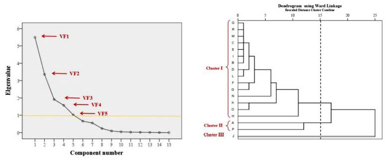
2.4.1. Factor Analysis

Factor analysis is a technique for reducing the dimension of a variable and it can be used for classifying a variable. Its purpose is to use a limited number of invisible hidden variables to explain the relationship between the original variables. It can extract less, non-correlated, abstract, and comprehensive indices from more than one measured original variable a called varifactor (VF). Each of the original variables can be represented by a linear combination of these extracted common factors. In addition, in accordance with the influence of each factor on the original variables, the original variables can be divided into a number of classes equal to the number of factors. The theoretical model for factor analysis is
z j i = a f 1 f 1 i + a f 2 f 2 i + a f 3 f 3 i + + a f m f m i + e f i
where
  • zji—the standardized score of variable j;
  • a—factor loading;
  • f—factor score;
  • m—number of common factors used for variables;
  • e—remainder of the error;
  • i—sample quantity;
  • j—number of variables.

2.4.2. Multivariate Linear Regression

Multivariate linear regression is a statistical analysis method used to determine the quantitative relationship between two or more variables using regression analysis in mathematical statistics. It can be predicted or estimated based on an optimal combination of multiple independent variables. The multivariate linear regression model is
Y = β 0 + β 1 X 1 i + β 2 X 2 i + + β k X k i + μ i
where
  • k—number of explanatory variables;
  • βK—partial regression coefficient;
  • β0—constant;
  • X—independent variable;
  • µ—random error.
Although factor analysis can reduce the number of variables and simplify the problem, it cannot determine the absolute contributions of various emission sources. The independent factors extracted by factor analysis represent different sources, with the factor score as the variable of the multiple linear regression. Nevertheless, the contribution of the emission source to the receptor can be calculated [12].

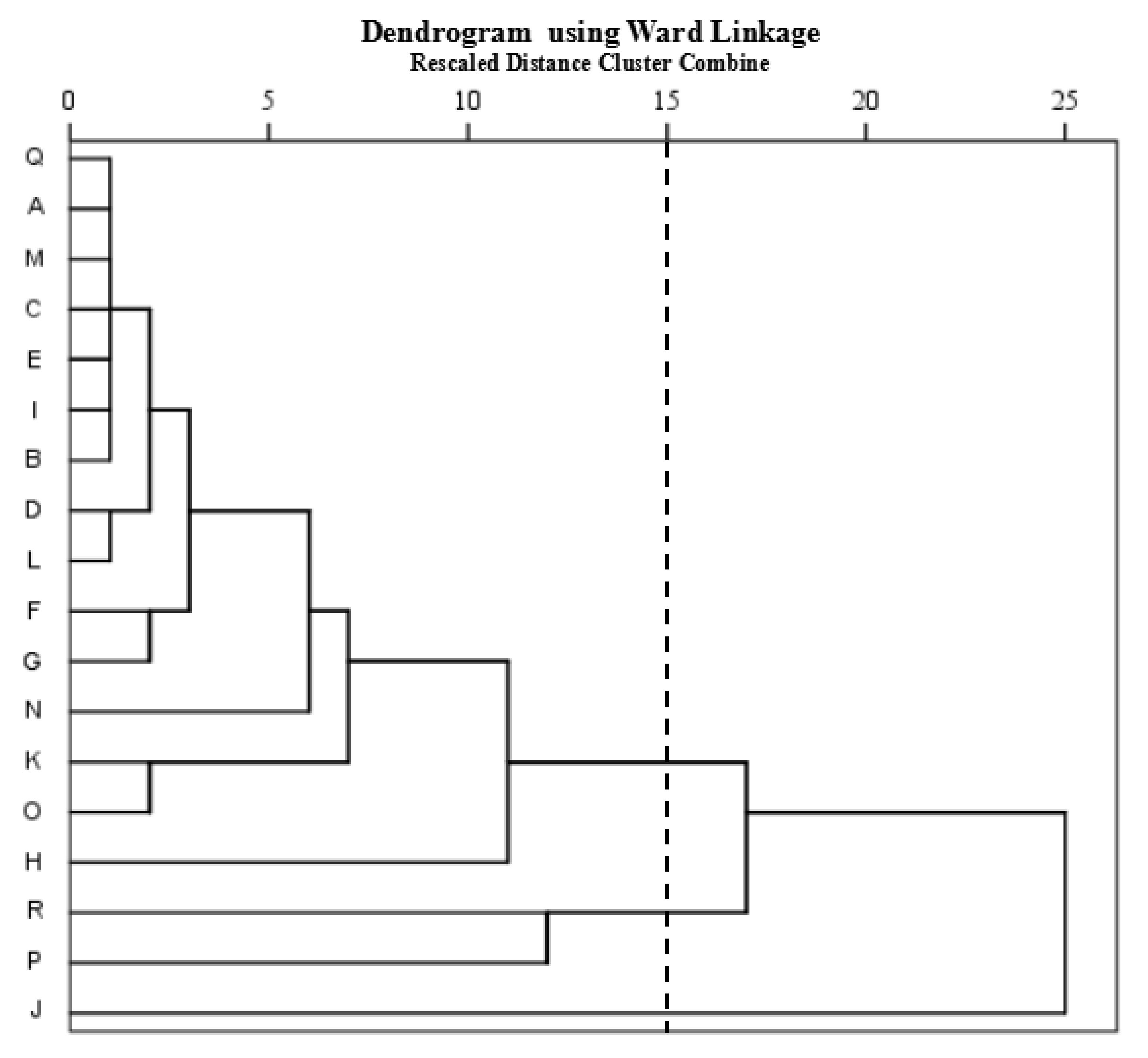
2.4.3. Cluster Analysis

Cluster analysis is a method for grouping objects into classes based on similarity within and between classes. The results of cluster analysis can help both in the interpretation of the data and in indicating patterns [13]. In hierarchical clustering, clusters are formed sequentially by starting with the most similar pair of objects and then forming subsequent higher clusters in a step-by-step process. In this study, hierarchical agglomerative cluster analysis was performed on the normalized dataset following Ward’s method using squared Euclidean distances as the measure of similarity [14].

3. Results and Discussion

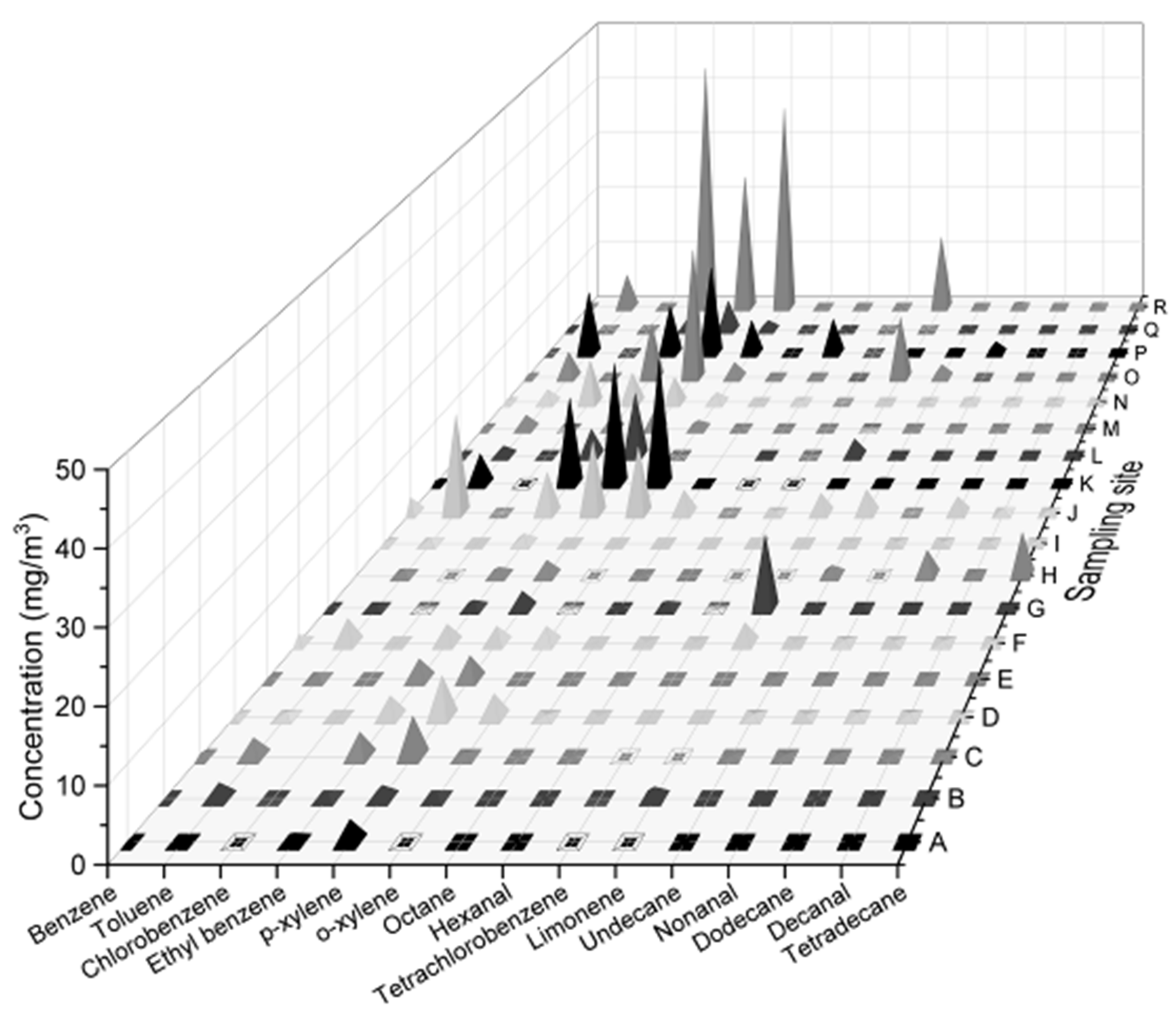
3.1. Level of Pollutants at Ship Sampling Sites

Figure 1 shows the 15 chemical pollutants that were detected at the 18 sampling sites onboard the bulk carrier ship. According to Material Safety Data Sheets [15], some of the chemical pollutants are moderately and weakly toxic substances, and although they are not included in the Chinese National Standards, their potential impact on human health should be taken seriously [16,17,18]. Benzene, toluene, ethylbenzene, p-xylene, and o-xylene were detected at each sampling site. The xylene concentration at sampling site R was more than the maximum limit (30 mg/m3; GJB 11.2-1991). The concentrations of benzene and xylene at other sampling sites did not exceed the maximum limit, although they were found with high concentrations near the comfort concentration limit (0.8 and 4.5 mg/m3, respectively; GJB 11.2-1991), suggesting that long-term release of these substances could potentially be harmful to crew health.

3.2. Pollution Source Apportionment at the Sampling Sites

In accordance with the distribution of organic components at the different sampling sites, an initial analysis of air pollution sources at the various locations was undertaken using a receptor model based on the multivariate statistical method. First, all data were standardized with a mean of 0 and variance of 1. Before undertaking the factor analysis, a Kaiser-Meyer-Olkin (KMO) test and a Bartlett spherical test were performed. The KMO test, which is used to check the degree of correlation and partial correlation between variables, has values between 0 and 1. The closer the KMO statistic is to 1, the stronger the correlation between variables, the weaker the partial correlation, and the more effective the factor analysis. If the Bartlett spherical test determines that the correlation array is a unit array, then the independent factor analysis method for each variable is invalid. As shown in Table 2, the value of KMO was 0.307 and the Bartlett test showed significance (p < 0.05), indicating that the parameters of these samples were suitable for factor analysis.
The KMO criterion was adopted to decide the appropriate number of factors to be retained (i.e., only those factors with eigenvalues >1) [19]. An eigenvalue of 1 would mean that the component could explain the variability of one variable. Therefore, according to this criterion, a component should be capable of explaining the variability of at least one variable. In a very large dimensional dataset, including components capable of explaining the variability of only one variable might not be very useful. As shown in Table 3, five common factors were extracted according to the criterion of having a feature value >1. The five common factors listed in Table 3 explained 89.092% of the total variance (cumulative contribution rate reached 90%), indicating that the characteristics of the original air pollution data could be well represented. The results suggest five major sources of air pollution at the 18 sampling sites.
The rotating composition matrix was obtained though orthogonal rotation (Table 4). Factor loadings >0.75, between 0.5 and 0.75, and between 0.3 and 0.5 are considered strong, moderate, and weak, respectively [20]. Our results showed the first common factor had strong positive loadings on benzene, toluene, octane, tetrachlorobenzene, undecane, and decanal, and moderate positive loadings on p-xylene, o-xylene, and dodecane. It has been reported that benzene, toluene, ethylbenzene, p-xylene, o-xylene, and other volatile benzene compounds are the principal constituents of paint and coatings [21,22]. Octane, undecane, dodecane, and decane are also common components of paint and coatings [23]. Therefore, the first common factor might be explained by the volatilization of paint and coatings on the ship. The second common factor had strong positive loading on ethylbenzene and moderate positive loadings on p-xylene, o-xylene, hexanal, limonene, and nonanal. Ethylbenzene is often found as a component of gasoline, and the mixture of p-xylene, m-xylene, and o-xylene can be used as a gasoline additive [24]. Previous studies have found that gasoline and diesel steam mainly include aromatic hydrocarbon, isomeric alkene, naphthene, n-alkane, and other volatile organic compounds [25,26,27]. Moreover, limonene can be used as a dispersant of oil. Therefore, it was deduced that the second common factor was explained by the volatilization of shipboard oil. The third common factor had moderate positive loadings on toluene and hexanal and weak positive loading on nonylaldehyde. Studies have confirmed the exposure of cooks to benzene and toluene from biomass fuel combustion [28]. For example, Klein et al. [29] found that emissions from shallow frying, deep frying, and charbroiling comprise predominantly aldehydes of differing relative composition depending on the type of oil used. Therefore, it was inferred that the third common factor was caused by human activities such as cooking. The fourth common factor had strong positive loading on tetradecane and moderate positive loading on dodecane. Tetradecane can be used in rubber and organic synthesis of resin, and rubber is used widely onboard ships in applications including sealing parts of windows and doors, pipeline shock absorbers, bearings, and other mechanical parts. Dodecane is often used as the main raw material oil of many chemical products intended for daily use [30]. Thus, the fourth common factor could be explained by high-temperature release from rubber and the use of daily chemical products. The fifth common factor had strong positive loading on only chlorobenzene. Chlorobenzene is used widely in insect repellents, mildew treatment, and deodorization. It is the main component of the insecticide and deodorant used in the ship’s dump/toilet. Therefore, it is believed that the fifth common factor could be explained by the application of deodorant and insecticide.

3.3. Distribution of Sampling Site Pollution

Using factor analysis, the factor score of the common factor at each sampling point could be calculated. The factor score of each VF multiplied by its variance contribution rate extracts a common factor, which can then be weighted to obtain composite scores for each sampling site. For any sampling site, the larger the factor score, the more serious the pollution at that point [31]. It is seen from the scores that the pollution levels at the sampling points varied (Table S1). Our results show that the overall pollution levels at each sampling site were in the order J > P > R > K > O > N > H > F > L > G > D > C > E > M > B > Q > I > A. For the first common factor VF1, the sampling point at site J had the highest score, showing the effect of volatilization of paint and coatings to be strongest, followed by R, O, K, H, F, and D. For the second common factor VF2, volatilization of shipboard oil at sampling site R was highest, followed in descending order by sampling sites P, K, O, G, and L. The third factor VF3 was clearly caused by human activities such as cooking at sampling site P, followed by J, N, F, M, and C. For the fourth common factor VF4, the most obvious effect from high-temperature release of rubber components and the daily use of chemical products was found at sampling site H, followed in descending order by P, R, and K. The fifth common factor VF5 had the highest score at sampling site N, mainly from the application of deodorant and insecticide, followed by R and H.

3.4. Contribution Rates of Sampling Site Pollution Source

Multiple linear regression can be performed using the factor score as the independent variable and the standardized concentration at each sampling point as the dependent variable. From Table 5, we have the regression equation Z = 0.366F1 + 0.224F2 + 0.128F3 + 0.105F4 + 0.068F5 + 5.805 × 10⁻⁷. It was determined that air pollution onboard the studied bulk carrier ship was affected by VF1, VF2, VF3, VF4, and VF5 and that their contribution rates were 41.07%, 25.14%, 14.37%, 11.78%, and 7.63%, respectively.

3.5. Classification of Sampling Site Pollution Levels

To implement control measures for the management of actual air pollution in ship compartments, in addition to factor analysis of the sources of compartment chemical pollutants, it is also necessary to develop a standard for the classification of the chemical pollutants. In this study, we further analyzed the spatial variations of air pollution and the degree of similarity between sampling sites using cluster analysis. The dendrogram obtained following Ward’s method, groups all 18 sampling sites into three statistically significant clusters (Figure 2). As in both Wang et al. [32] and Li et al. [33], the clustering procedure highlighted groups for which the sites had similar characteristics and natural source types. In our study, the hierarchical clustering analysis grouped the sampling sites into three clusters with similar air pollution characteristics. Cluster I (sampling sites A–I, K–O, and Q) corresponds to sampling sites with relatively weak pollution. Cluster II (sampling sites P and R) corresponds to sampling sites with moderate pollution Cluster III (sampling site J) corresponds to strong pollution and it represents a sampling site influenced primarily by the volatilization of paint and coatings and by human activities such as cooking. The extracted group information could be used to reduce the number of sampling sites in further study without significant loss of information.

4. Conclusions

The present study investigated the compartmental air pollution that occurred during the voyage of the large oceangoing ship. Factor analysis helped identify the factors/sources responsible for the variation of air pollution in different compartments. The VFs obtained from factor analysis indicated there were five common factors responsible for the variation of air pollution. Receptor modeling using multivariate linear regression analysis showed the contributions to air pollution of these five common factors, i.e., the volatilization of ship paint, volatilization of ship-based oil, cooking activities, high-temperature release of rubber components on the ship and daily use of chemical products, and the application of deodorant and insecticide, were 41.07%, 25.14%, 14.37%, 11.78%, and 7.63%, respectively. Furthermore, hierarchical clustering analysis grouped the sampling sites into three clusters with similar air pollution characteristics. The extracted group information could be used to reduce the number of sampling sites in further studies without significant loss of information. The findings of this study highlight the usefulness of multivariate statistical techniques in the identification and apportionment of pollution sources/factors, which can reveal crucial information regarding air pollution during the voyage of a large oceangoing ship.

Limitations and Future Research

This study explored pollution sources only from the perspective of multivariate statistics. The methods adopted in this research should be verified further with other case studies. Some air pollution variables are known to receive contributions from unidentified sources; thus, further work will be necessary in order for them to be identified.

Supplementary Materials

The following are available online at https://0-www-mdpi-com.brum.beds.ac.uk/1660-4601/16/3/389/s1, Table S1. Common factors and comprehensive scores of different sampling sites.

Author Contributions

Q.W. conceived and designed the experiments and wrote the paper; D.A. and R.S. performed the experiments and contributed reagents and analysis tools; M.S. analyzed the data.

Funding

This research was funded by the Army Logistics Research Plan of China (BHJ15J004 and AP14C001).

Acknowledgments

The authors thank Steven Hunter, M.S., from Liwen Bianji, Edanz Group China (www.liwenbianji.cn/ac), for editing the English text of a draft of this manuscript.

Conflicts of Interest

The authors declare no conflict of interest.

References

  1. Fang, J.; He, Y.; Xu, L.; Pan, H.; Xu, X. Analysis of volatile compounds in the closed ship cabins. Ship. Sci. Technol. 2013, 35, 90–95. [Google Scholar]
  2. Shen, Z.; Wang, X.; Li, H.; Huang, J.; Mo, F.; Shen, H. Investigation of subjective evaluation to cabin air quality in vessels. Occup. Health. 2016, 32, 104–105. [Google Scholar]
  3. Elskus, A.A.; Ingersoll, C.G.; Kemble, N.E.; Echols, K.R.; Brumbaugh, W.G.; Henquinet, J.W.; Watten, B.J. Real-time analysis of organic compounds in ship engine aerosol emissions using resonance-enhanced multiphoton ionisation and proton transfer mass spectrometry. Anal. Bioanal. Chem. 2015, 407, 5939–5951. [Google Scholar]
  4. Oeder, S.; Kanashova, T.; Sippula, O.; Sapcariu, S.C.; Streibel, T.; Arteaga-Salas, J.M.; Passig, J.; Dilger, M.; Paur, H.R.; Schlager, C.; et al. Particulate matter from both heavy fuel oil and diesel fuel shipping emissions show strong biological effects on human lung cells at realistic and comparable in vitro exposure conditions. PLoS. ONE 2015, 10, e0126536. [Google Scholar] [CrossRef] [PubMed]
  5. Streibel, T.; Schnelle-Kreis, J.; Czech, H.; Harndorf, H.; Jakobi, G.; Jokiniemi, J.; Karg, E.; Lintelmann, J.; Matuschek, G.; Michalke, B.; et al. Aerosol emissions of a ship diesel engine operated with diesel fuel or heavy fuel oil. Environ. Sci. Pollut. Res. Int. 2017, 24, 10976–10991. [Google Scholar] [CrossRef] [PubMed]
  6. Xu, D.; Yu, T.; Chen, L.; Zhou, A.; Shen, X. Advances on the evaluation methods of ship nonmetallic material emission property and measurement. Chin. J. Ship. Research. 2015, 10, 113–120. [Google Scholar]
  7. NRC. Submarine Air Quality; National Academy Press: Washington, DC, USA, 1988. [Google Scholar]
  8. Mccarrick, A. Measurements of monoethanolamine near a US navy carbon dioxide scrubber. In Proceedings of the 40th International Conference on Environmental Systems, Barcelona, Spain, 11–15 July 2010; ARC: Reston, VA, USA, 2010. [Google Scholar] [CrossRef]
  9. Sampson, H. International Seafarers and Transnationalism in the Twenty First Century; Manchester University Press: Manchester, UK, 2013. [Google Scholar]
  10. Gordon, G.E. Receptor models. Environ. Sci. Technol. 1980, 14, 792–800. [Google Scholar] [CrossRef]
  11. Hu, X.; Xu, X.; Ding, Z.; Chen, Y.; Lian, H.Z. In vitro inhalation/ingestion bioaccessibility, health risks, and source appointment of airborne particle-bound elements trapped in room air conditioner filters. Environ. Sci. Pollut. Res. Int. 2018, 25, 26059–26068. [Google Scholar] [CrossRef]
  12. Li, S.; Li, J.; Zhang, Q. Water quality assessment in the rivers along the water conveyance system of the Middle Route of the South to North Water Transfer Project (China) using multivariate statistical techniques and receptor modeling. J. Hazard. Mater. 2011, 195, 306–317. [Google Scholar] [CrossRef]
  13. Singh, K.P.; Malik, A.; Mohan, D.; Sinha, S. Multivariate statistical techniques for the evaluation of spatial and temporal variations in water quality of Gomti River (India)—A case study. Water. Res. 2004, 38, 3980–3992. [Google Scholar] [CrossRef]
  14. Otto, M. Multivariate Methods. In Analytical Chemistry; Kellner, R., Mermet, J.M., Otto, M., Widmer, H.M., Eds.; Wiley: Weinheim, Germany, 1998; p. 916. [Google Scholar]
  15. Material Safety Data Sheets. Available online: http://cheman.chemnet.com/en-msds.html (accessed on 10 December 2018).[Green Version]
  16. Gustafson, D.L.; Long, M.E.; Thomas, R.S.; Benjamin, S.A.; Yang, R.S. Comparative hepatocarcinogenicity of hexachlorobenzene, pentachlorobenzene, 1,2,4,5-tetrachlorobenzene, and 1,4-dichlorobenzene: application of a medium-term liver focus bioassay and molecular and cellular indices. Toxicol. Sci. 2000, 53, 245–252. [Google Scholar] [CrossRef] [PubMed]
  17. Vaghef, H.; Hellman, B. Demonstration of chlorobenzene-induced DNA damage in mouse lymphocytes using the single cell gel electrophoresis assay. Toxicology 1995, 96, 19–28. [Google Scholar] [CrossRef]
  18. Saghir, S.A.; Zhang, F.; Rick, D.L.; Kan, L.; Bus, J.S.; Bartels, M.J. In vitro metabolism and covalent binding of ethylbenzene to microsomal protein as a possible mechanism of ethylbenzene-induced mouse lung tumorigenesis. Regul. Toxicol. Pharmacol. 2010, 57, 129–135. [Google Scholar] [CrossRef] [PubMed]
  19. Kaiser, H.F. The varimax criterion for analytic rotation in factor analysis. Psychometrika 1958, 32, 443–482. [Google Scholar] [CrossRef]
  20. Liu, C.W.; Lin, K.H.; Kuo, Y.M. Application of factor analysis in the assessment of ground water quality in a Blackfoot disease area in Taiwan. Sci. Total. Environ. 2003, 313, 77–89. [Google Scholar] [CrossRef]
  21. Liu, M.; Yang, X.; Wang, L.; Zhang, Z. Determination of benzene series compounds in oil paints by Internal Standard Method using GC/MS. Environ. Sci. Technol. 2011, 34, 135–138. [Google Scholar]
  22. Zhou, J.; Wang, X.; Cao, H.; Mao, Y.; Zhou, G. Benzene series in oil paint thinners determined by gas chromatography. Environ. Sci. Technol. 2007, 30, 19–21. [Google Scholar]
  23. Schweitzer, P.A. Paintings and Coatings: Applications and Corrosion Resistance; CRC Press: Boca Raton, FL, USA, 2006. [Google Scholar]
  24. Heibati, B.; Godri; Pollitt, K.J.; Charati, J.Y.; Ducatman, A.; Shokrzadeh, M.; Karimi, A.; Mohammadyan, M. Biomonitoring-based exposure assessment of benzene, toluene, ethylbenzene and xylene among workers at petroleum distribution facilities. Ecotoxicol. Environ. Saf. 2018, 149, 19–25. [Google Scholar] [CrossRef]
  25. Li, C.; Wang, Y.; Tian, S. Relationship between gasoline composition and calculated octane number distribution according to boiling range. Acta. Petrolei. Sinica. 2017, 33, 138–143. [Google Scholar]
  26. Lu, S.H.; Bai, Y.H.; Zhang, G.S.; Ma, J. Study on the characteristics of VOCs source profiles of vehicle exhaust and gasoline emission. Acta. Scientiarum. Naturalium. Universitatis. Pekinensis. 2003, 39, 507–511. [Google Scholar]
  27. Wu, Y.T.; Yang, G.F.; Wang, G.; Xu, C.M.; Shen, B.J.; Gao, J.S. Effect of reaction temperature on the catalytic pyrolysis of gasoline for the favored production of light olefins. Modern. Chemical. Industry. 2009, 29, 74–77. [Google Scholar]
  28. Sinha, S.N.; Kulkarni, P.K.; Shah, S.H.; Desai, N.M.; Patel, G.M.; Mansuri, M.M.; Saiyed, H.N. Environmental monitoring of benzene and toluene produced in indoor air due to combustion of solid biomass fuels. Sci. Total Environ. 2006, 357, 280–287. [Google Scholar] [CrossRef] [PubMed]
  29. Klein, F.; Platt, S.M.; Farren, N.J.; Detournay, A.; Bruns, E.A.; Bozzetti, C.; Daellenbach, K.R.; Kilic, D.; Kumar, N.K.; Pieber, S.M.; et al. Characterization of Gas-Phase Organics Using Proton Transfer Reaction Time-of-Flight Mass Spectrometry: Cooking Emissions. Environ. Sci. Technol. 2016, 50, 1243–1250. [Google Scholar] [CrossRef] [PubMed]
  30. Förster, M.; Bolzinger, M.A.; Ach, D.; Montagnac, G.; Briançon, S. Ingredients tracking of cosmetic formulations in the skin: A confocal Raman microscopy investigation. Pharm. Res. 2011, 28, 858–872. [Google Scholar] [CrossRef]
  31. Sun, R.; An, D.; Lu, W.; Shi, Y.; Wang, L.; Zhang, C.; Zhang, P.; Qi, H.; Wang, Q. Impacts of a flash flood on drinking water quality: Case study of areas most affected by the 2012 Beijing flood. Heliyon 2016, 2, e00071. [Google Scholar] [CrossRef] [PubMed]
  32. Wang, X.; Cai, Q.; Ye, L.; Qu, X. Evaluation of spatial and temporal variation in stream water quality by multivariate statistical techniques: A case study of the Xiangxi River basin, China. Quatern. Int. 2012, 282, 137–144. [Google Scholar] [CrossRef] [Green Version]
  33. Li, S.; Zhang, Q. Response of dissolved trace metals to land use/land cover and their source apportionment using a receptor model in a subtropic river, China. J. Hazard. Mater. 2011, 190, 205–213. [Google Scholar] [CrossRef]
Figure 1. Average concentrations of 15 air pollutants at different sampling sites.
Ijerph 16 00389 g001
Figure 2. Dendrogram obtained using cluster analysis.
Ijerph 16 00389 g002
Table 1. Identification of the 18 sampling sites onboard the bulk carrier ship.
Sampling SiteLocationSampling SiteLocationSampling SiteLocation
AWheel houseGPastry roomMEngine control room
BCompartment 1HIncineration roomNShower room
CDining roomISwitching roomOCompartment 2
DAlley way 1JLavatoryPGalley
EEngine roomKStore roomQPump room
F CabinLAlley way 2RFuel oil tank
Table 2. Results of Kaiser–Meyer–Olkin (KMO) and Bartlett tests.
Kaiser–Meyer–Olkin measure of sampling adequacy0.307
Bartlett’s test of sphericityApprox. Chi-square342.816
df105
Sig.0.000
Table 3. Total variance explained.
ComponentInitial EigenvaluesExtraction Sums of Squared Loadings
Total% Of VarianceCumulative %Total% of VarianceCumulative %
15.49736.64936.6495.49736.64936.649
23.35522.36759.0153.35522.36759.015
31.91512.76371.7791.91512.76371.779
41.57610.50882.2871.57610.50882.287
51.0216.80589.0921.0216.80589.092
60.6594.39593.487
70.5533.68697.173
80.2361.57298.745
90.0910.60599.350
100.0420.28399.633
110.0240.16299.795
120.0180.11899.913
130.0110.07199.985
140.0020.01499.998
150.0000.002100.000
Table 4. Component matrix.
VariablesComponent
12345
Benzene0.804−0.4170.219−0.2370.023
Toluene0.8040.2230.5270.003−0.010
Chlorobenzene−0.125−0.0250.093−0.1410.948
Ethylbenzene0.4570.752−0.4120.0350.133
p-xylene0.5150.698−0.1090.080−0.076
o-xylene0.5610.647−0.360−0.0010.102
Octane0.862−0.3070.266−0.205−0.003
Hexanal−0.0850.5620.7090.390−0.030
Tetrachlorobenzene0.870−0.1330.164−0.282−0.003
Limonene0.3680.518−0.377−0.078−0.174
Undecane0.845−0.2170.2280.165−0.080
Nonanal−0.1310.7480.4960.2270.122
Dodecane0.613−0.475−0.1550.6010.087
Decanal0.791−0.059−0.399−0.0240.144
Tetradecane0.159−0.356−0.2110.8790.084
Table 5. Regression coefficients of multiple regression equation.
ModelNon-Standardized CoefficientStandardized Coefficient
BStandard ErrorBeta
Constant5.805 × 10−70.000
F10.3660.0000.788
F20.2240.0000.481
F30.1280.0000.274
F40.1050.0000.226
F50.0680.0000.146

