Assessment of Ecosystem Service Quality and Its Correlation with Landscape Patterns in Haidian District, Beijing

Abstract
:
1. Introduction
2. Materials and Methods
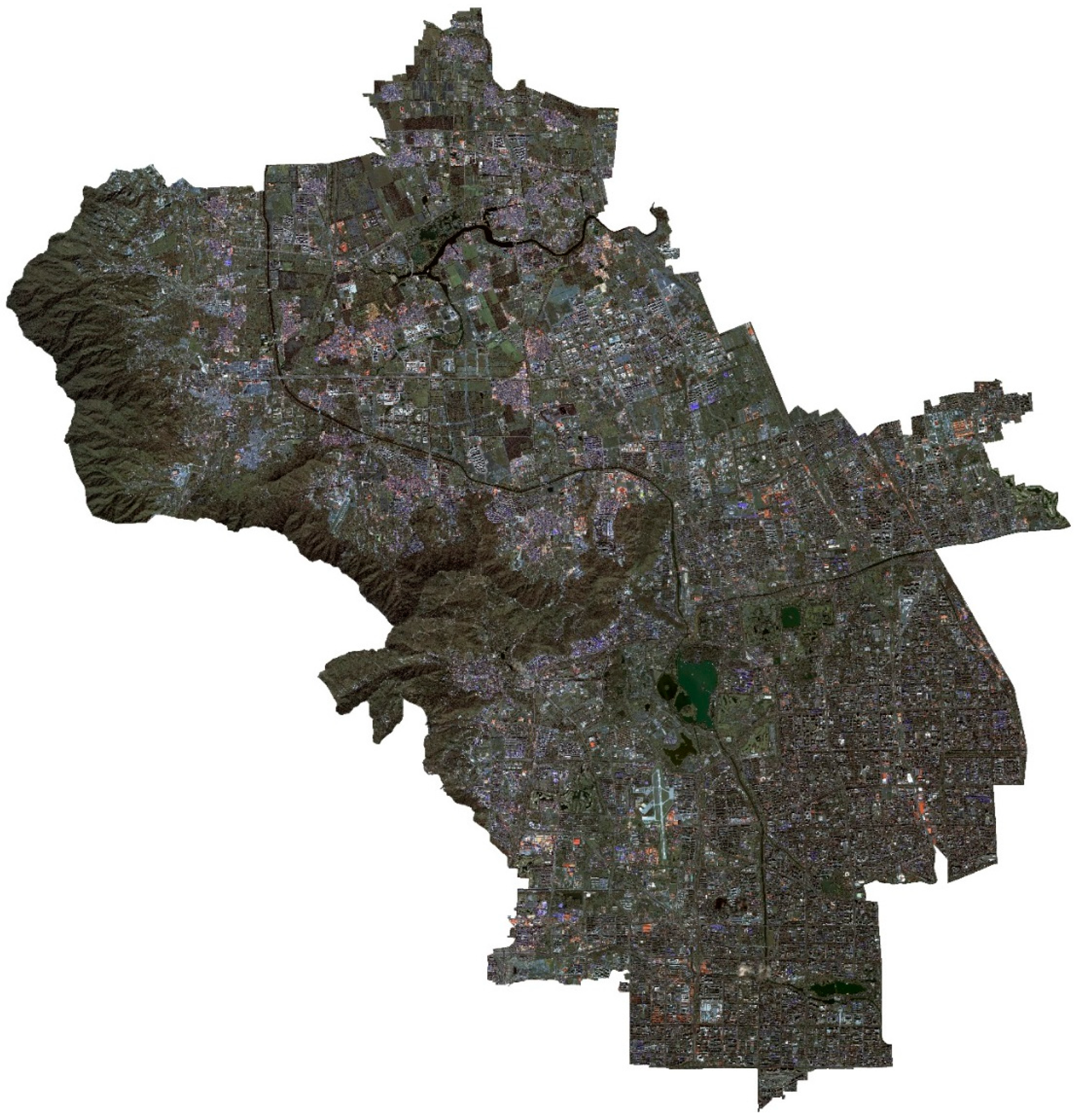
2.1. Haidian District Overview
2.2. Method
2.2.1. Data Sources and Processing
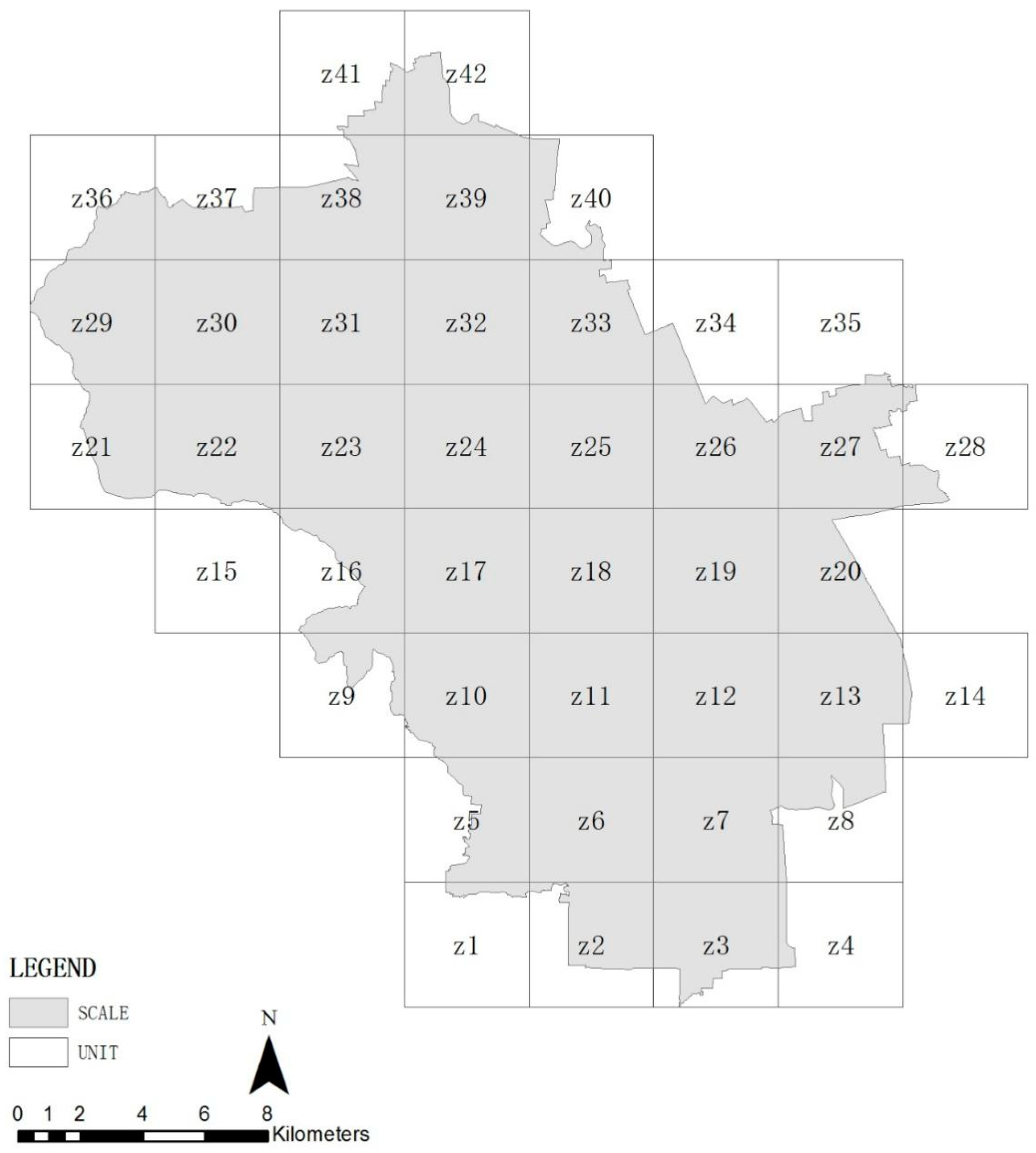
2.2.2. Division of Research Units
2.2.3. Computing Method of Ecosystem Service Quality
2.2.4. Computing Method of Landscape Pattern
3. Results
3.1. Quality of Ecosystem Services in Haidian District
3.1.1. Total Service Quality of Ecosystem Service
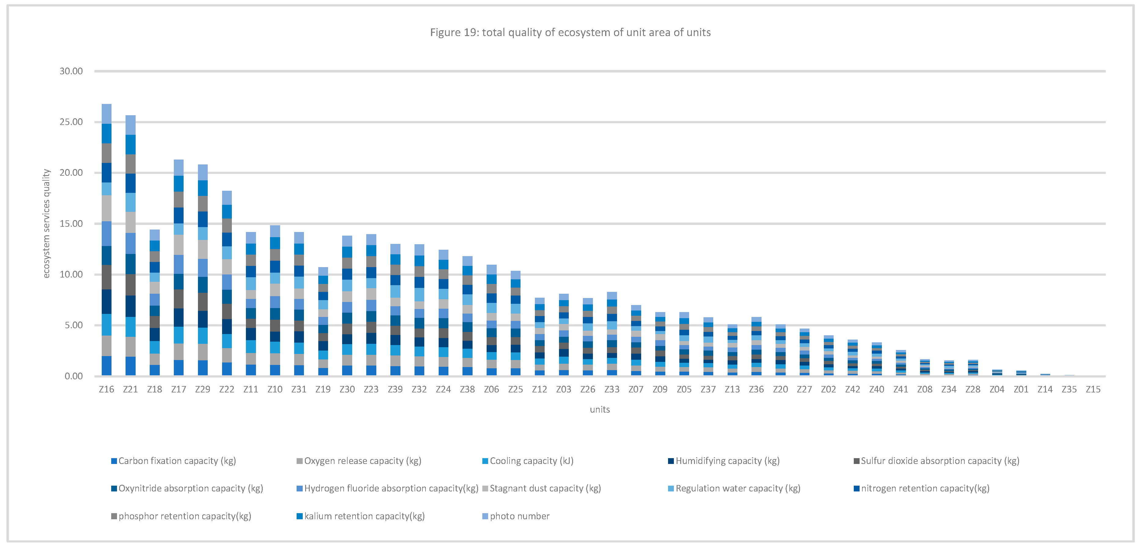
3.1.2. Quality of Ecosystem Service in Unit Area of Research Units
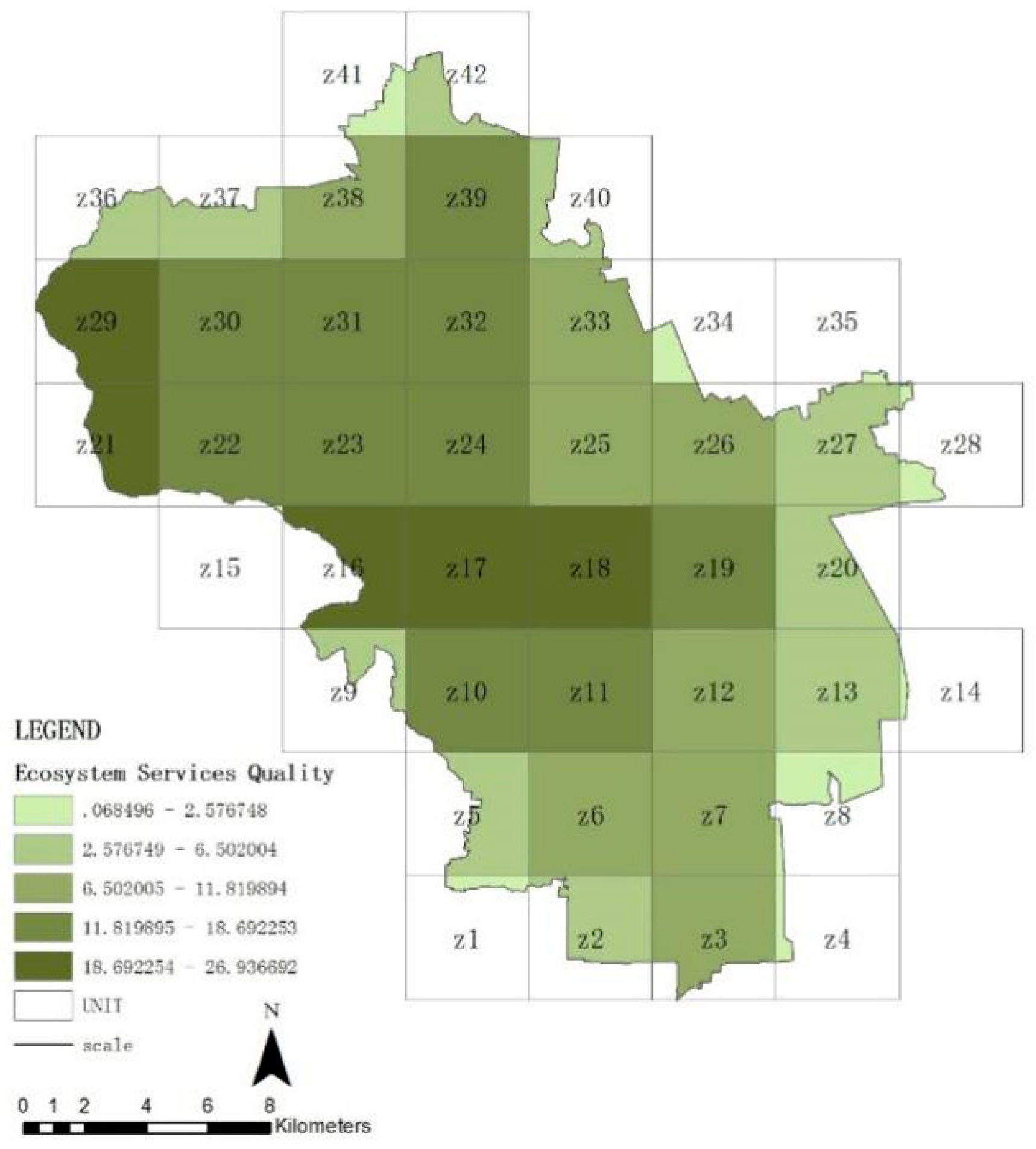
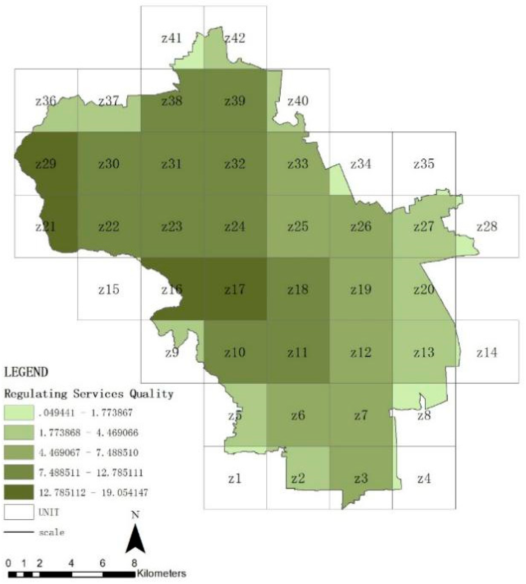
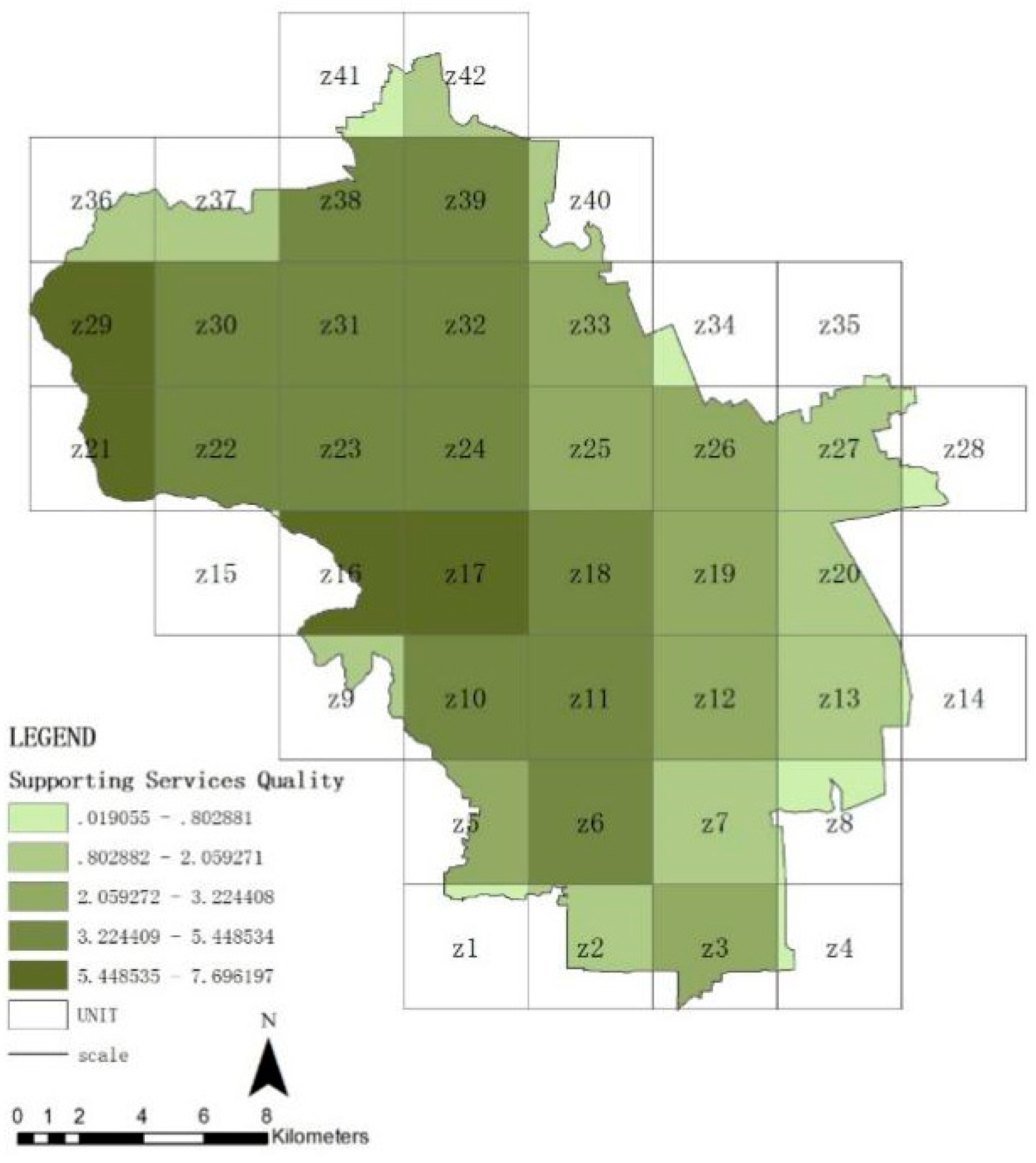
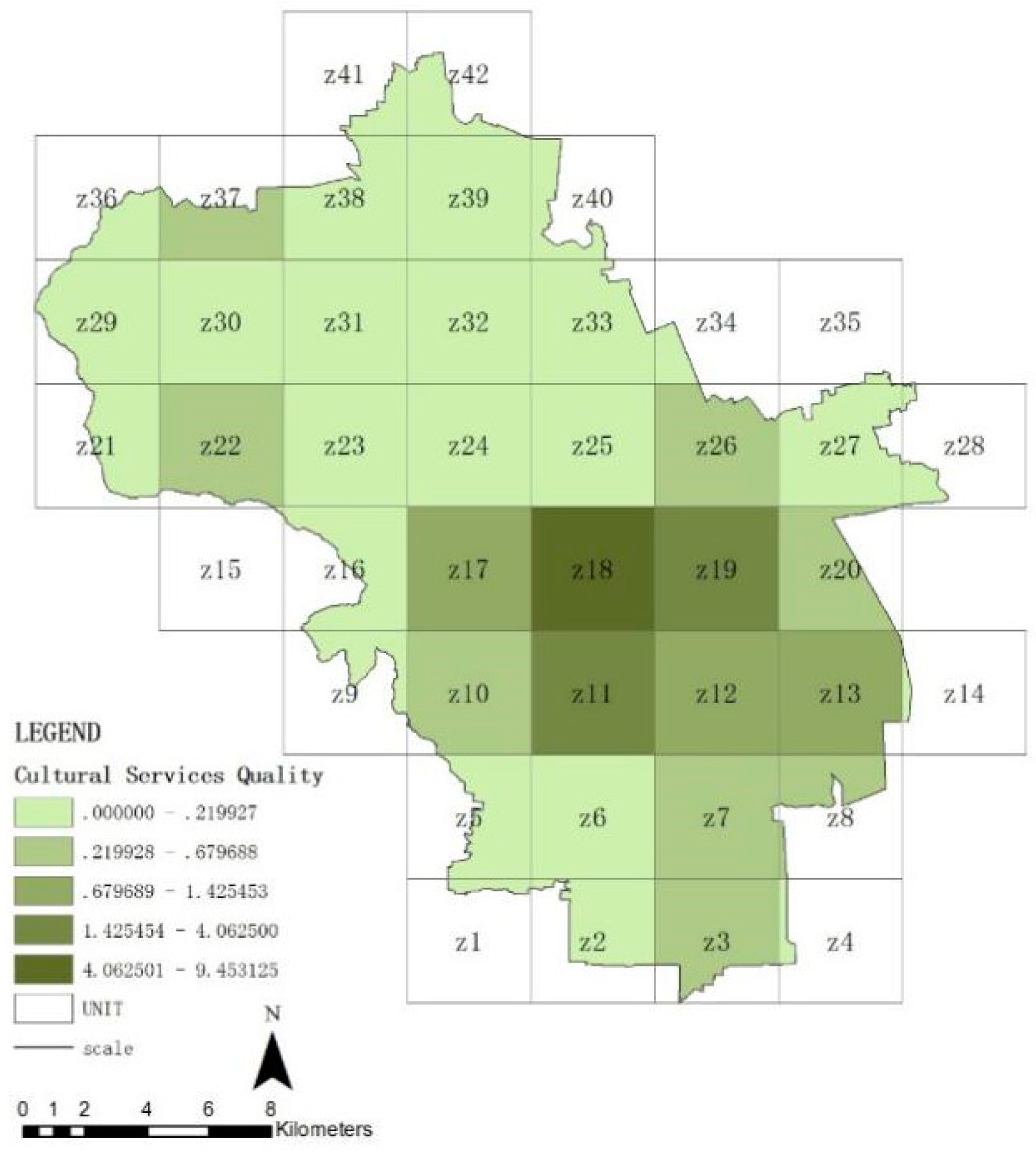
3.2. Spatial Distribution Features of Ecosystem Service in Haidian District
3.3. Analysis of the Association between the Landscape Pattern and Quality of the Ecosystem Service in Haidian District
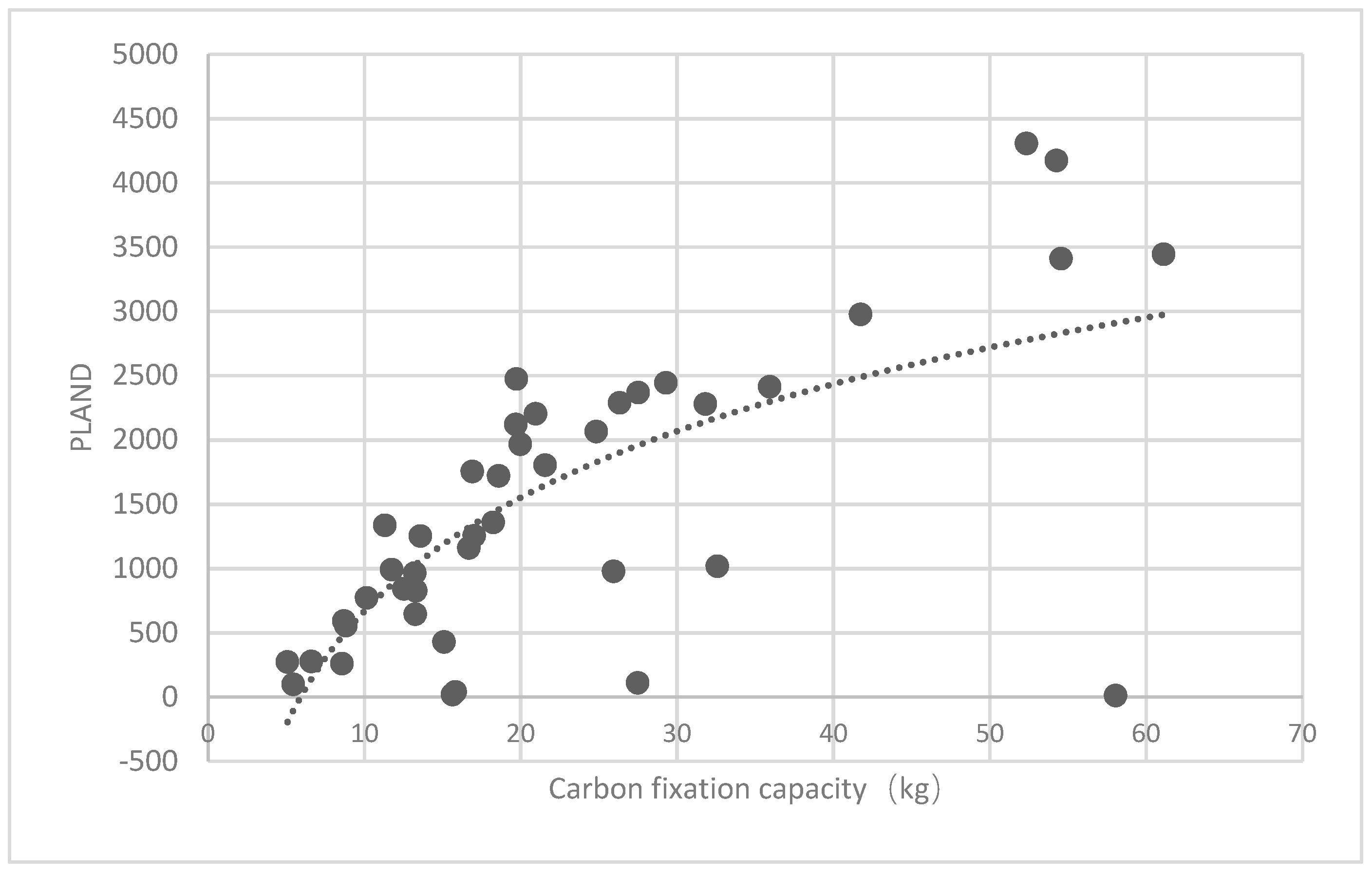
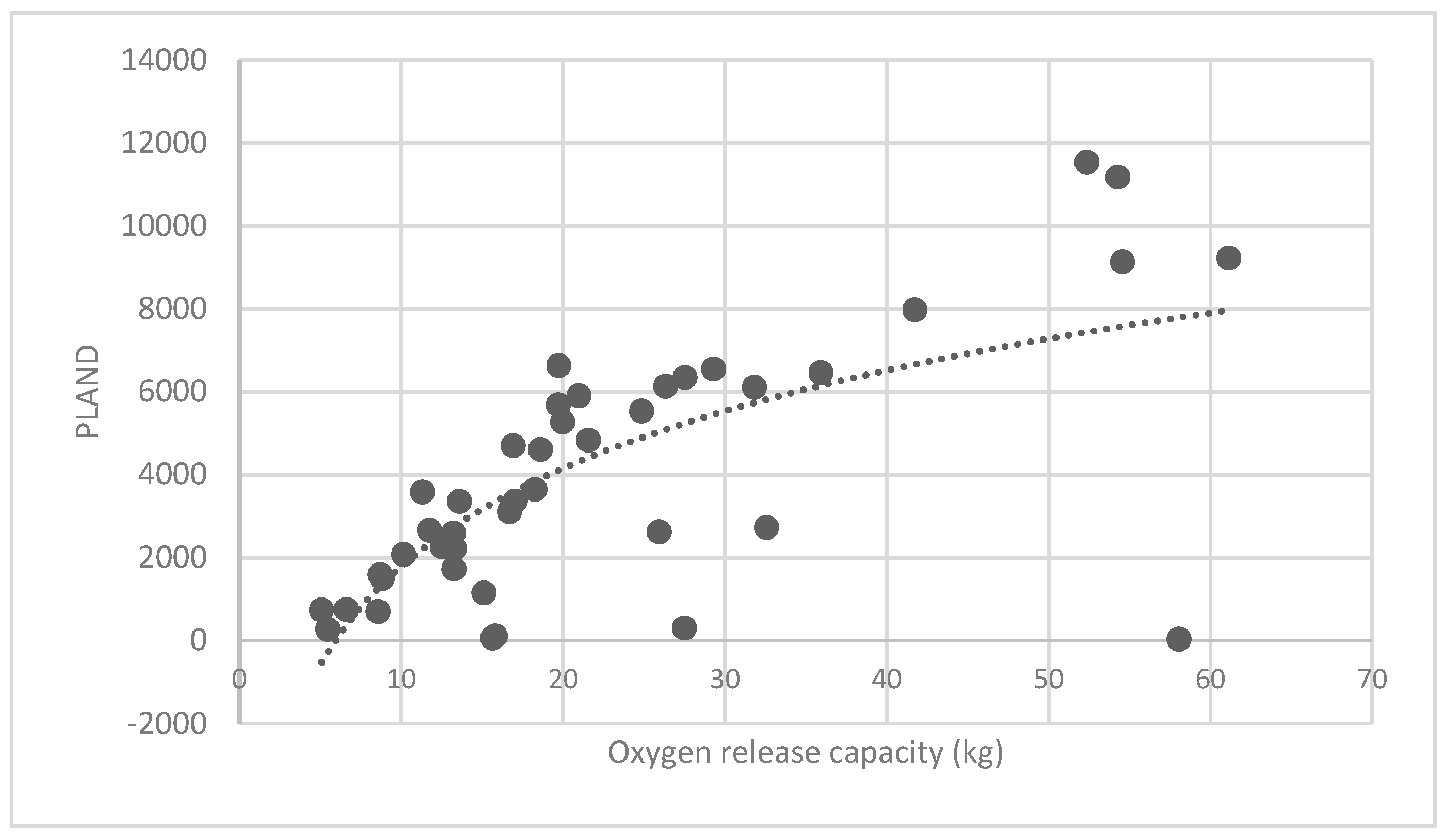
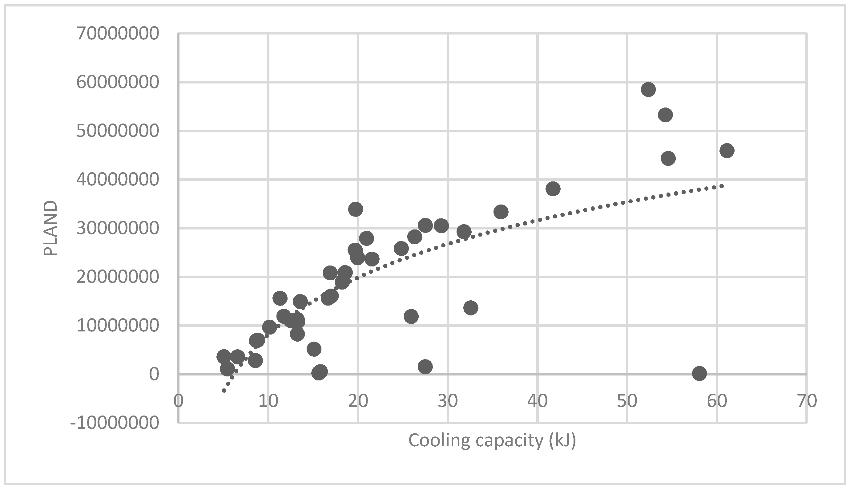
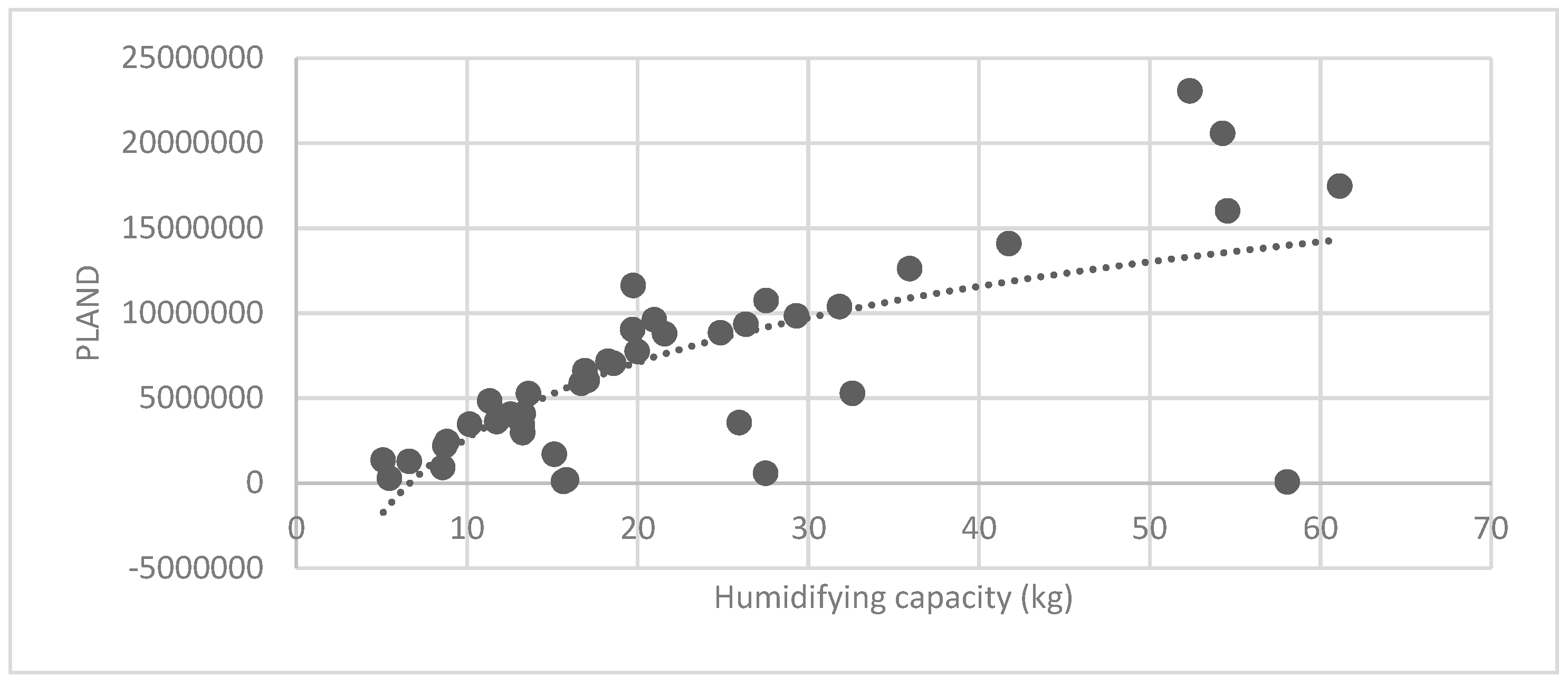
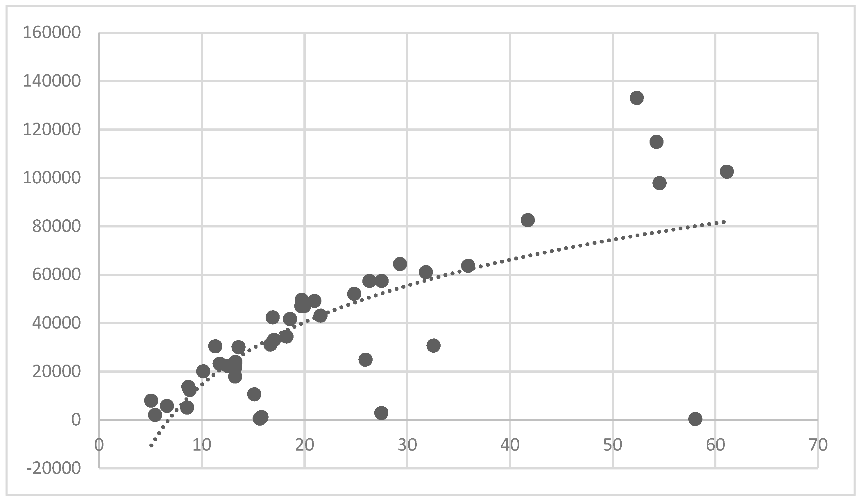
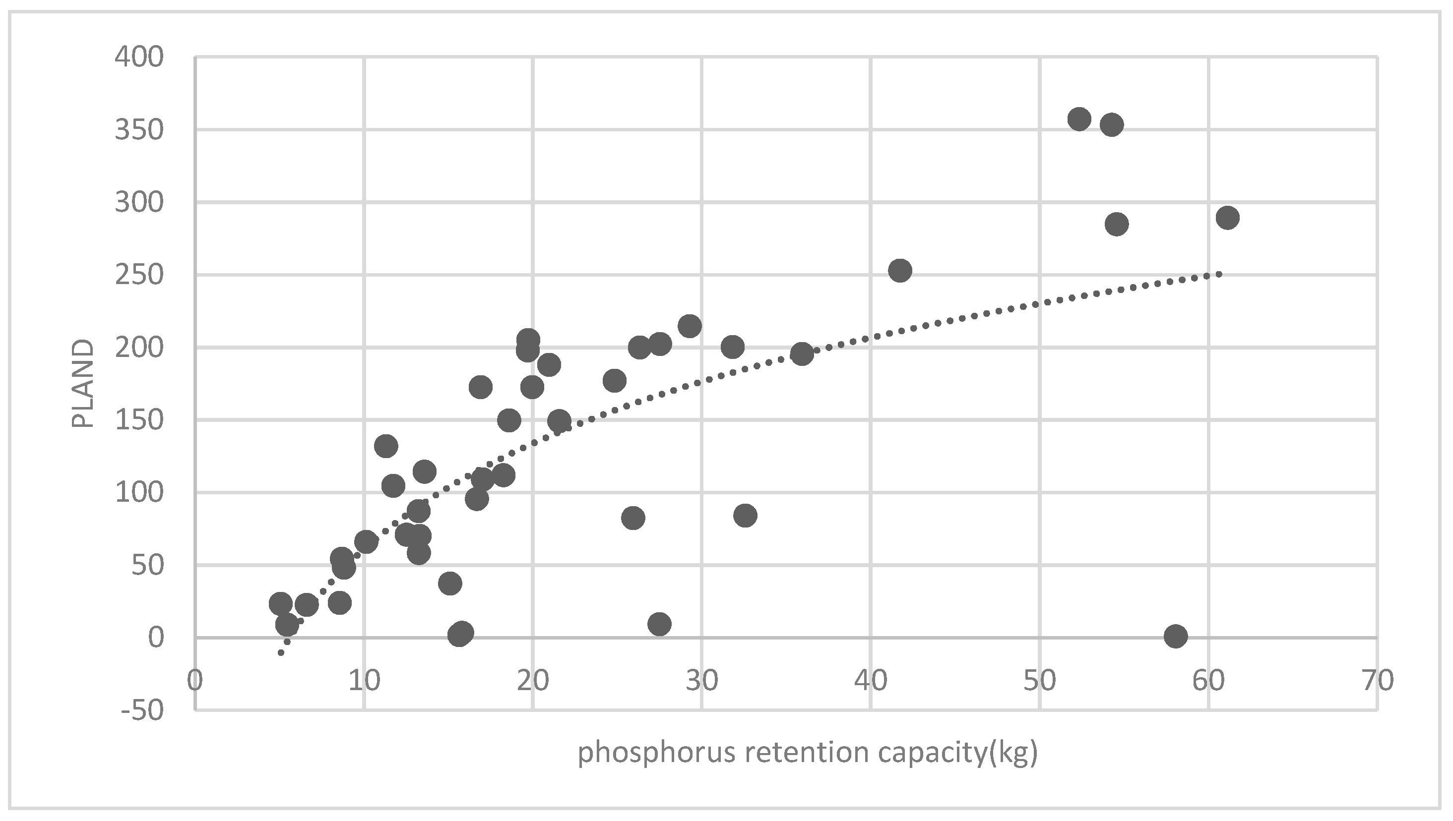
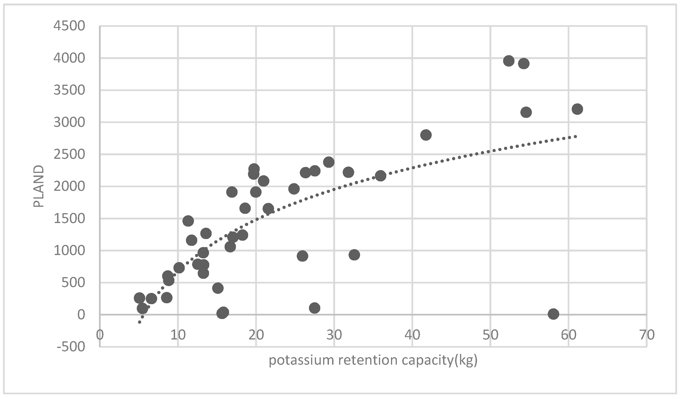
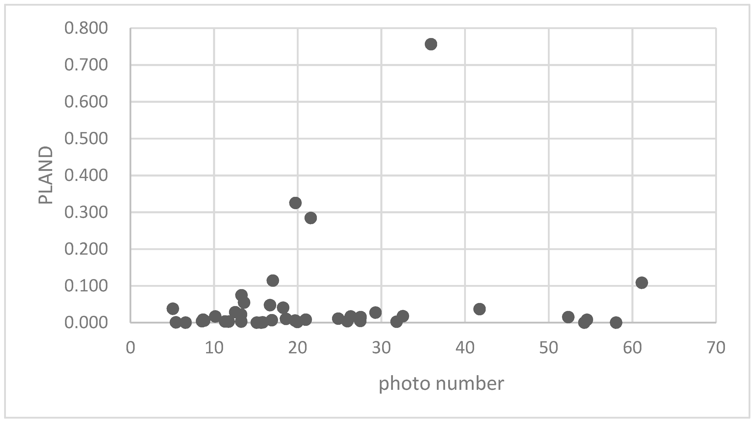
3.3.1. Analysis of the Association of the Percentage of Patches (PLAND) Index of Forest Land and Quality of Ecosystem Service in Haidian District
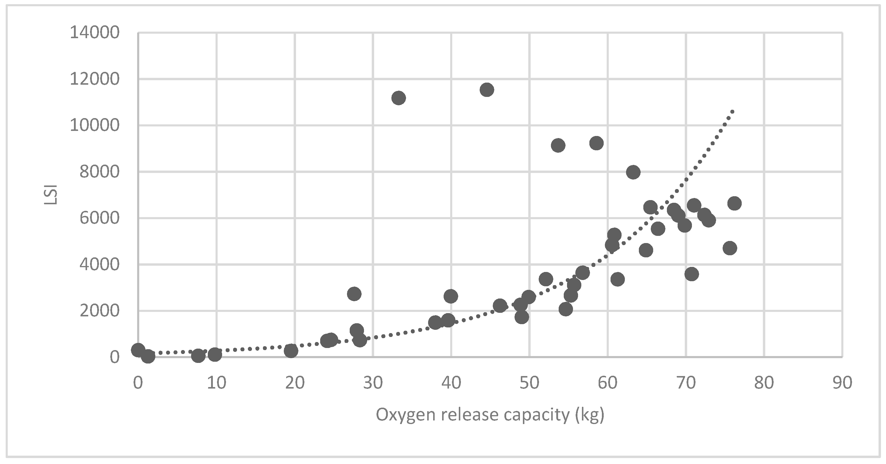
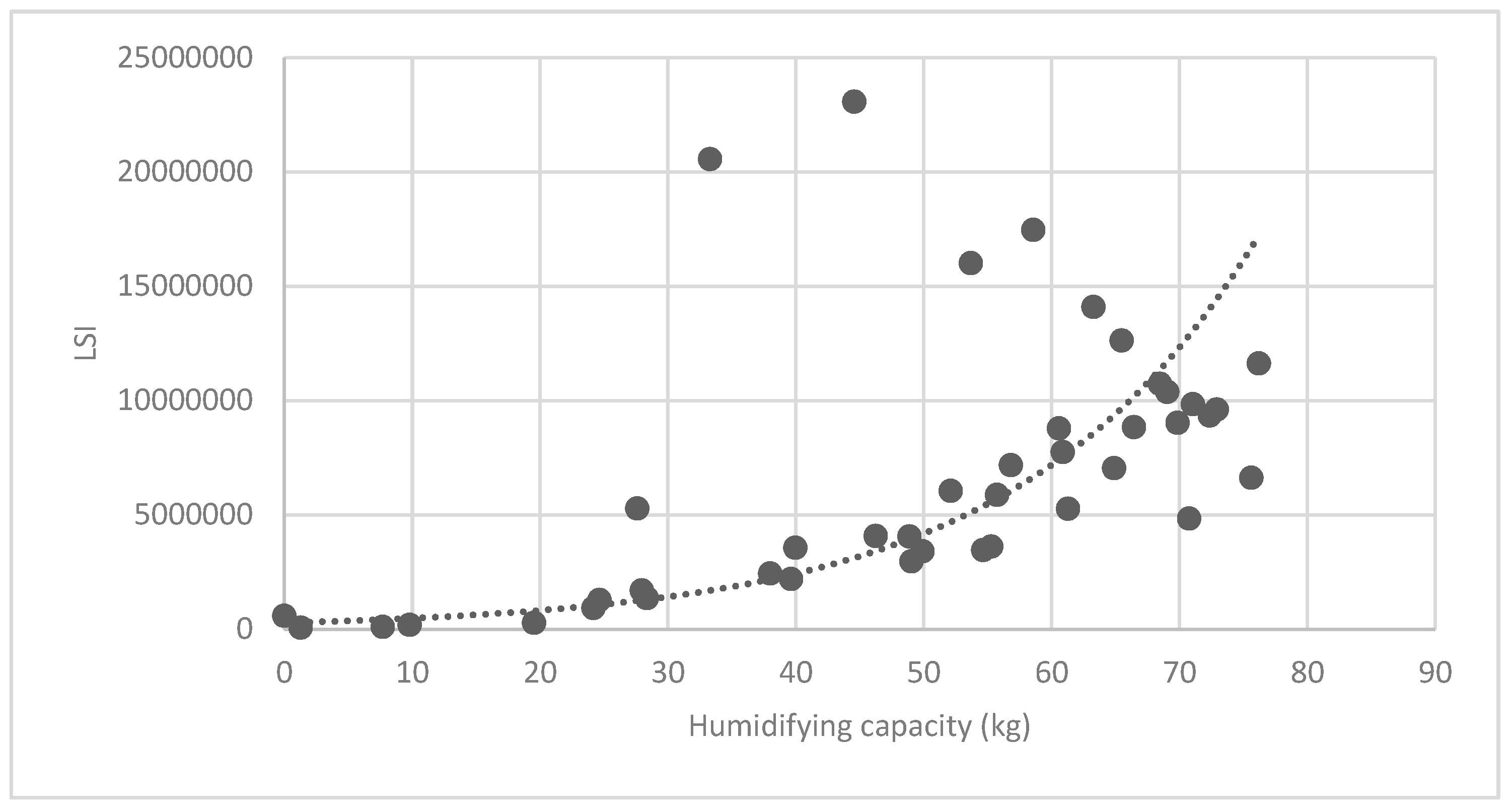
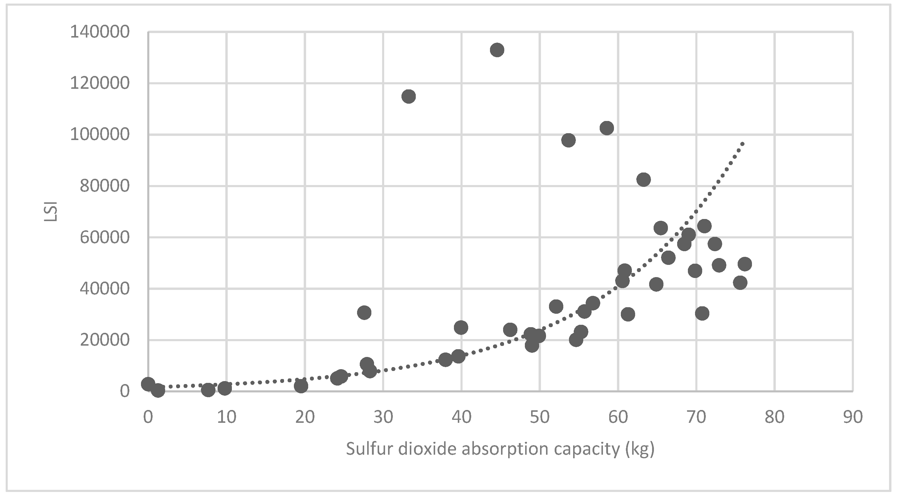
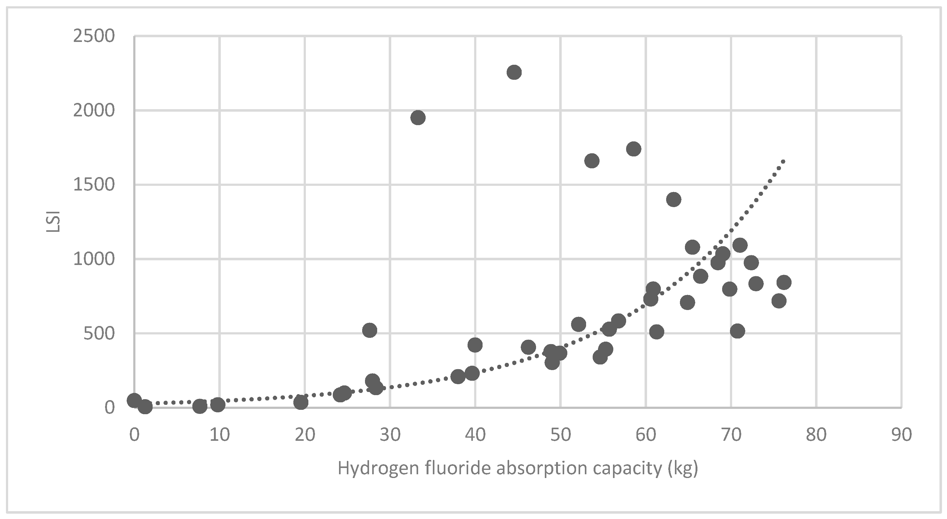
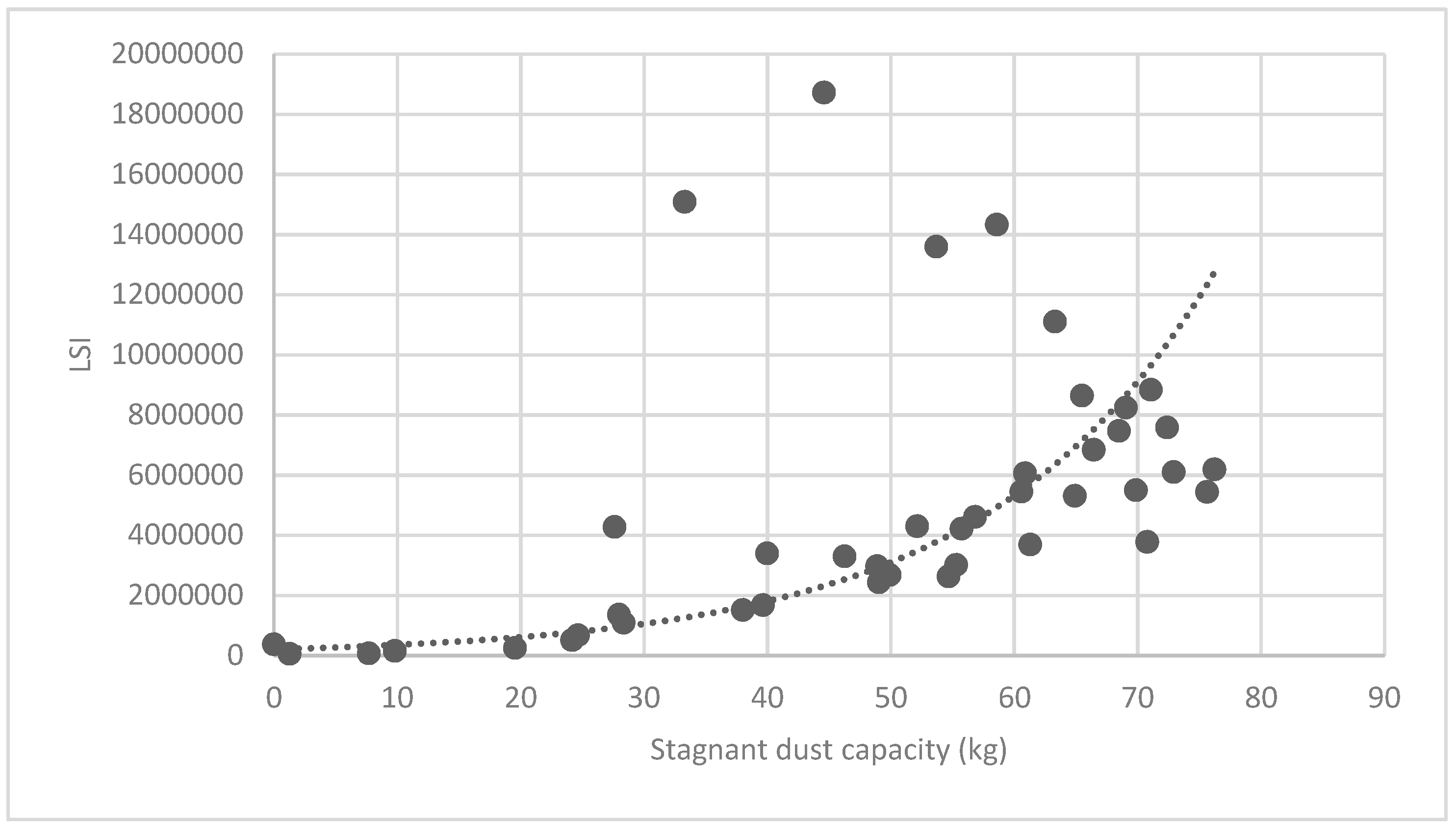
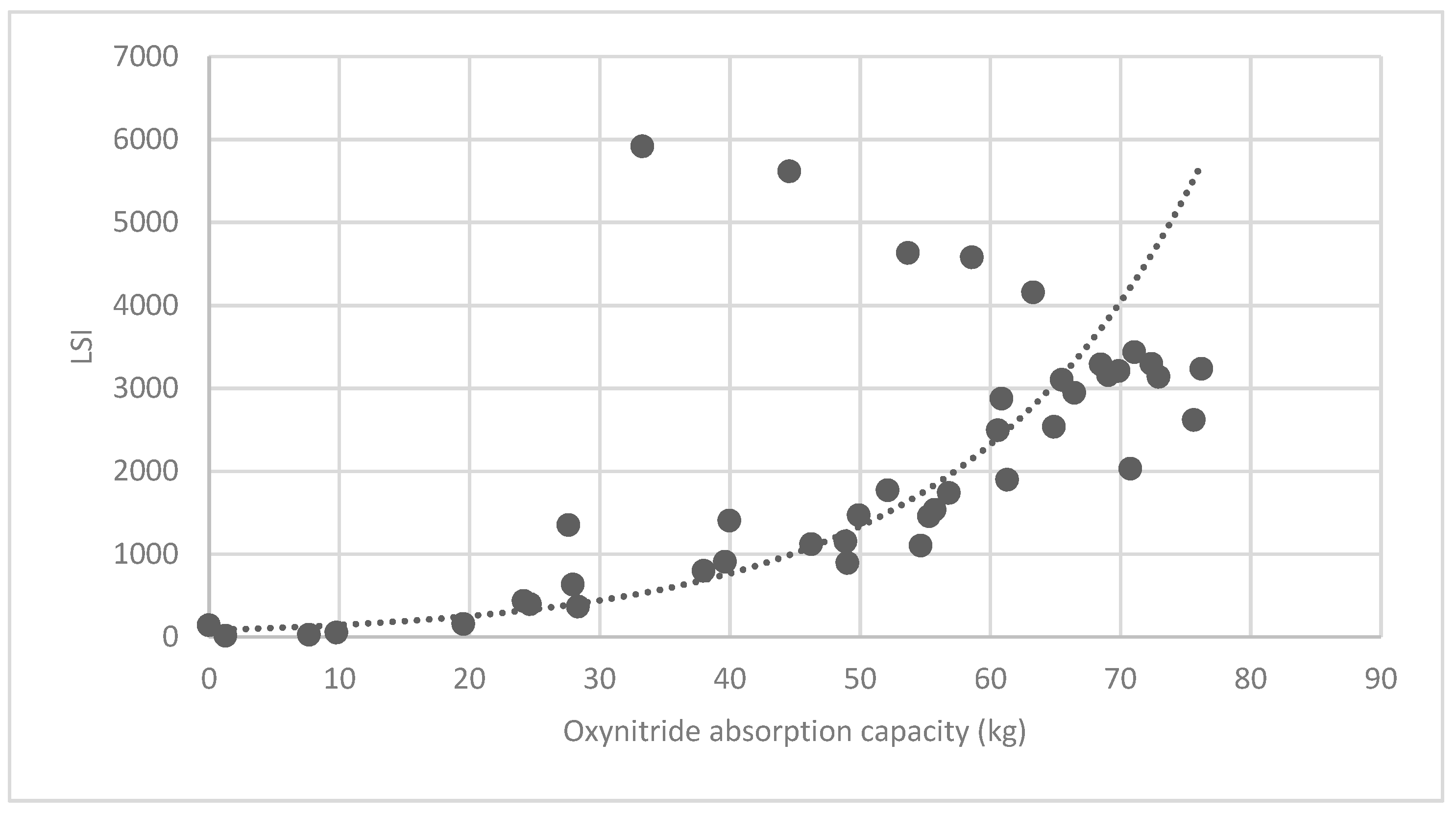
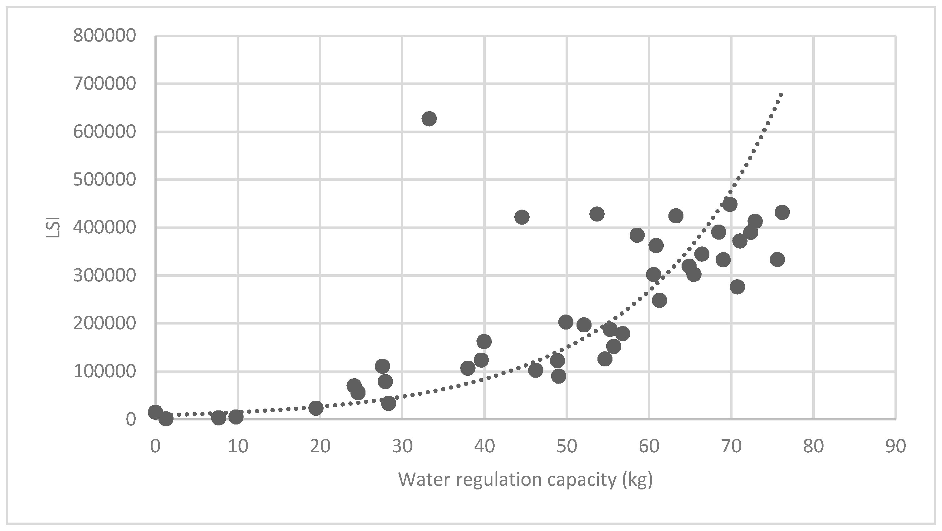
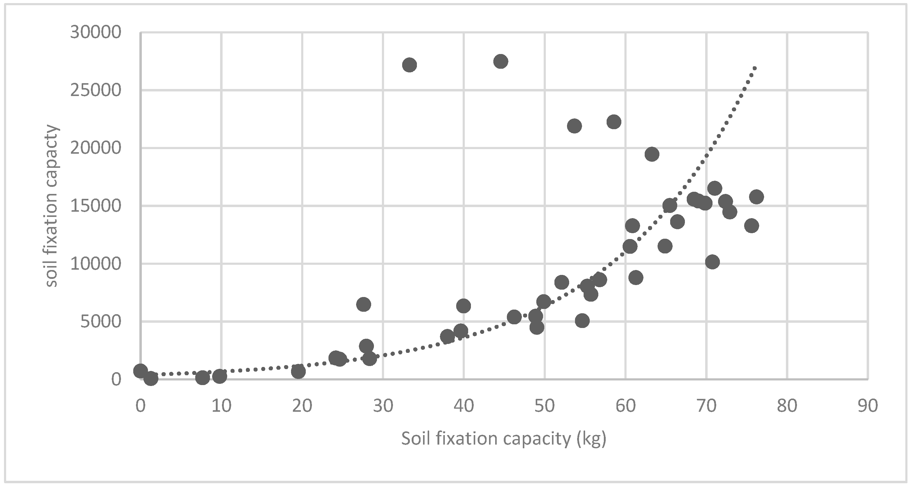
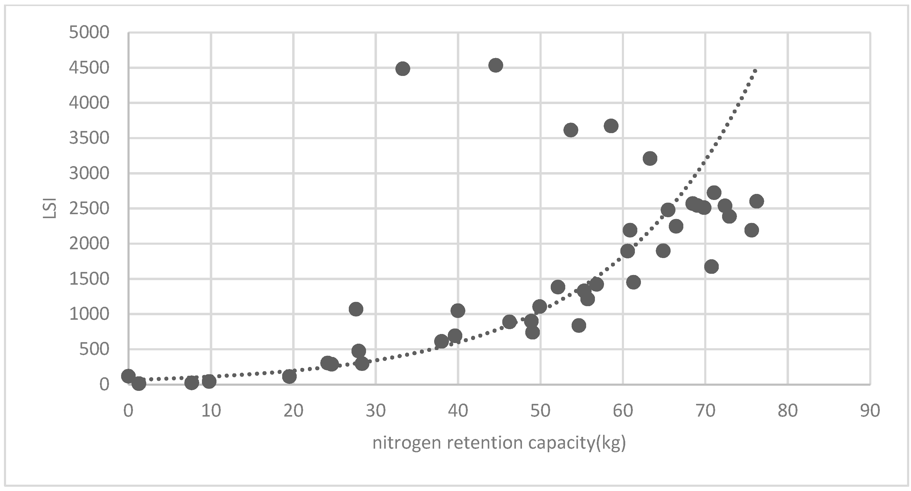
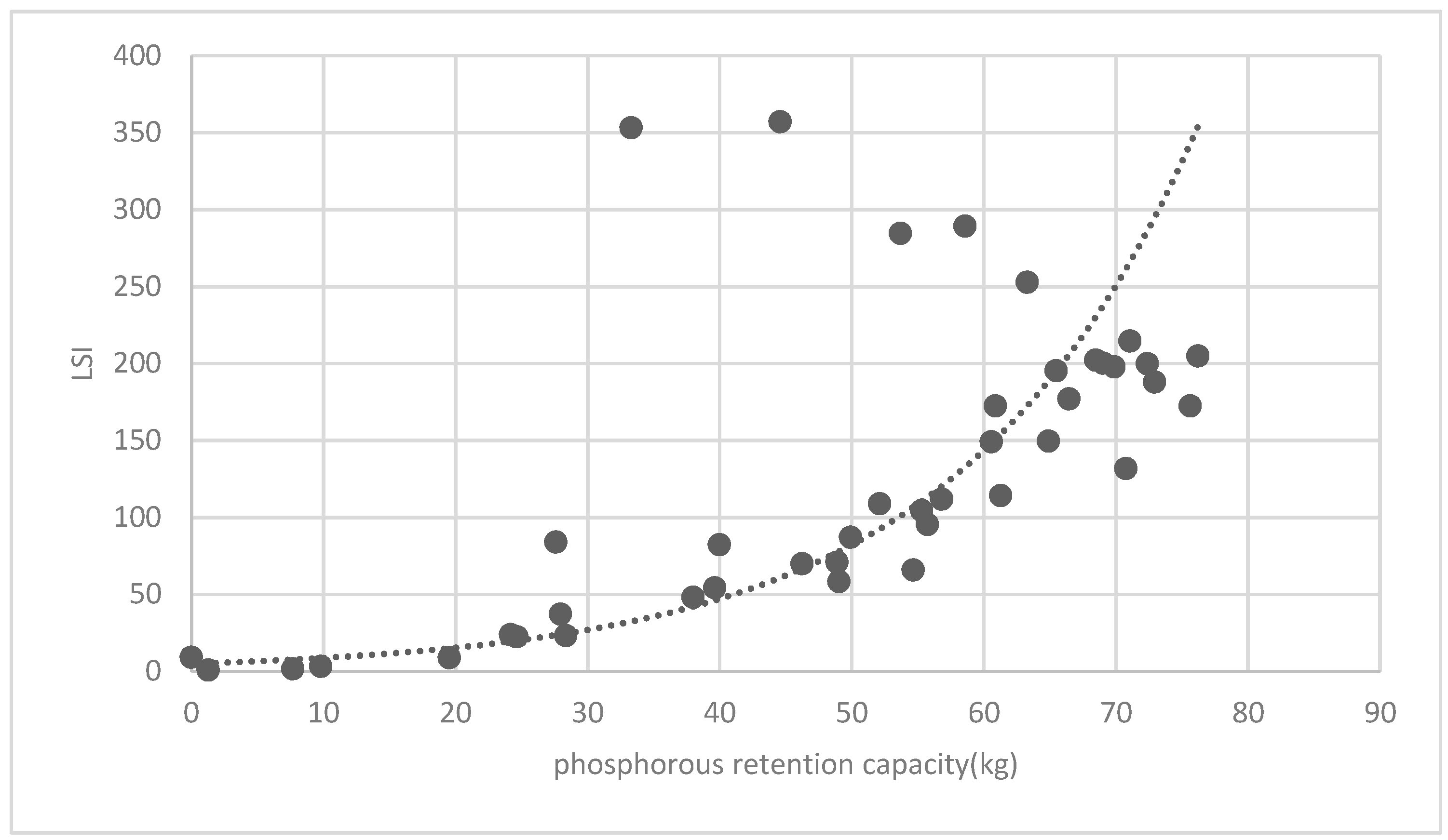
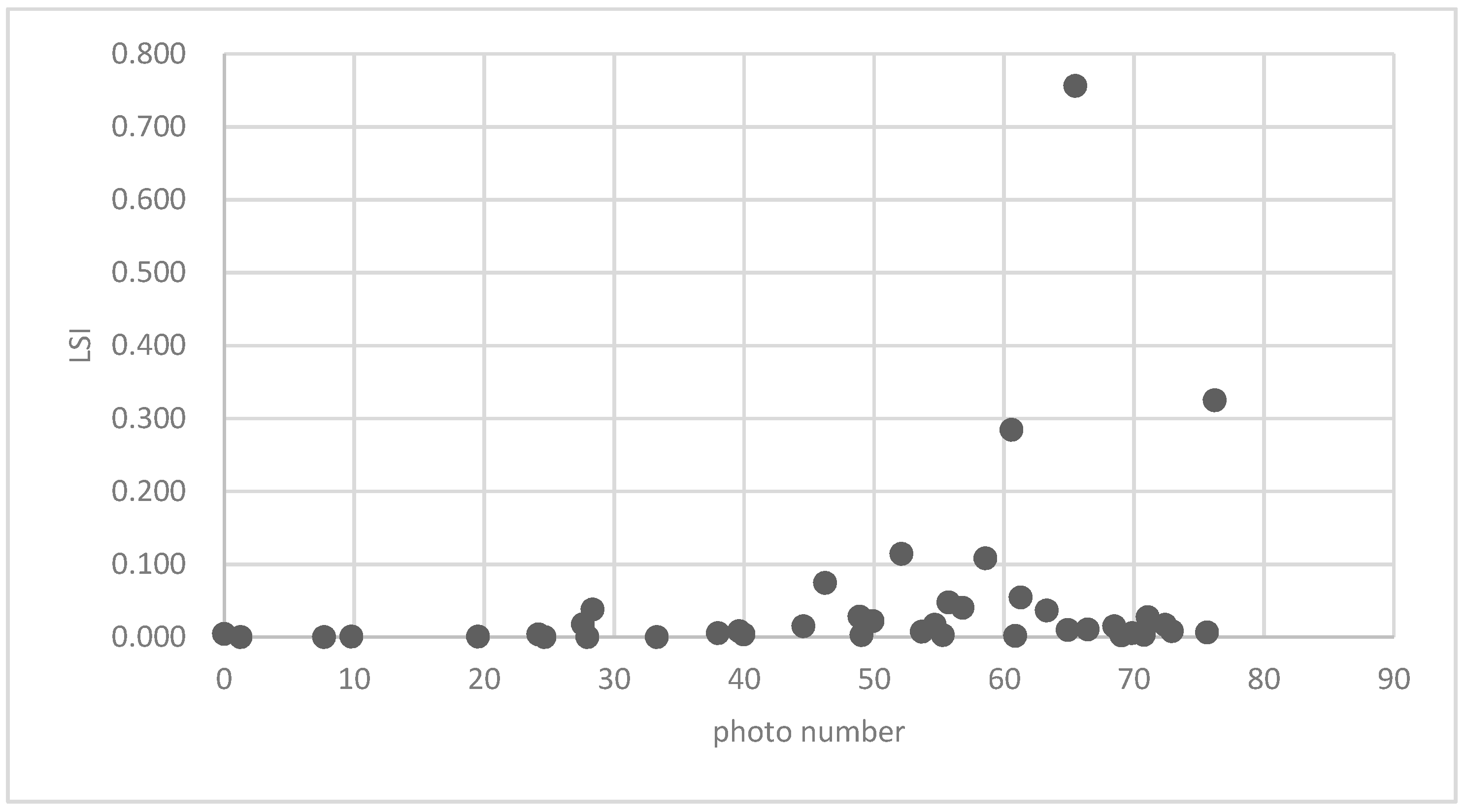
3.3.2. Analysis of Landscape Shape Index (LSI) of Brush and Quality of Ecosystem Service in Haidian District
4. Discussion
4.1. Association between Landscape Pattern and Ecosystem Service
4.2. Optimization Strategy of Green Space in Haidian District
5. Conclusions
- (1)
- The research results show that forest land is the main provider of the ecosystem service in Haidian District, while construction land only provides cultural service. For the total quality of the unit area of the ecosystem service, the quality of units Z10, Z11, Z16, Z17, Z18, Z19, Z21, Z22, Z29, and Z31 is higher than the quality of unit Z30 approximates the whole average in Haidian District;
- (2)
- On the whole, the ecosystem service spaces of Haidian District are divided into the western mountainous area, the northern plain, and the southwestern urban area, and decrease from the west to the east. These are roughly matched with the spatial distribution of the forest land. The regulating service and supporting service are maximum in the western mountainous area, followed by the northern plain. The southwestern urban area has the minimal regulating service and supporting service. This is consistent with the distribution of the urban green space. The cultural service capabilities in the research unit where there are important historical cultural resources in Haidian District—namely, the “Three Hills and Five Parks”—are far stronger than those of other areas. Therefore, the cultural service is closely associated with the historical resource points;
- (3)
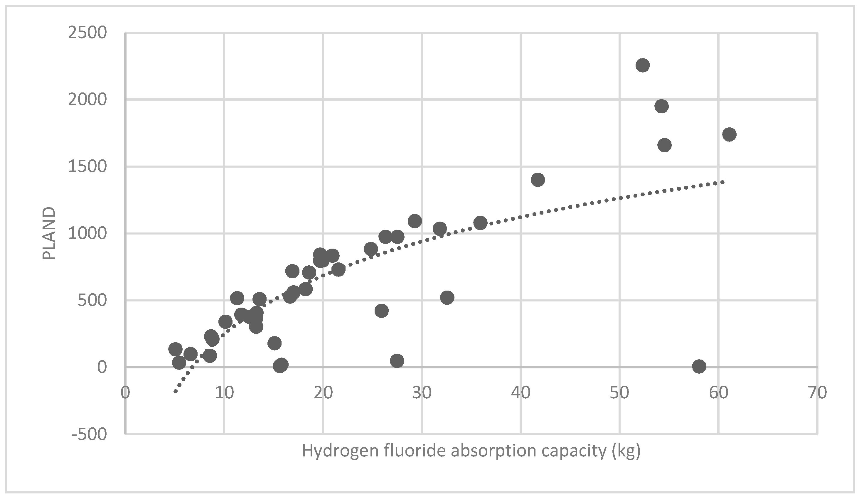
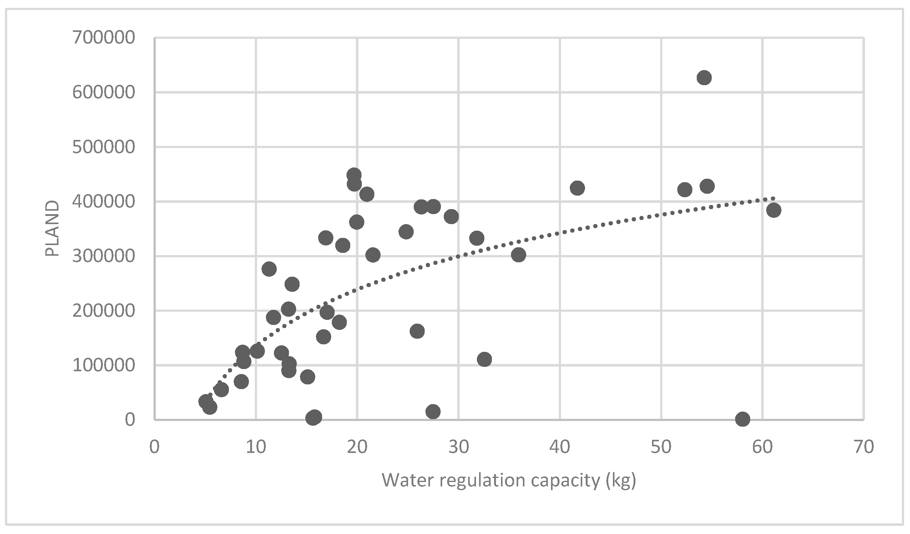
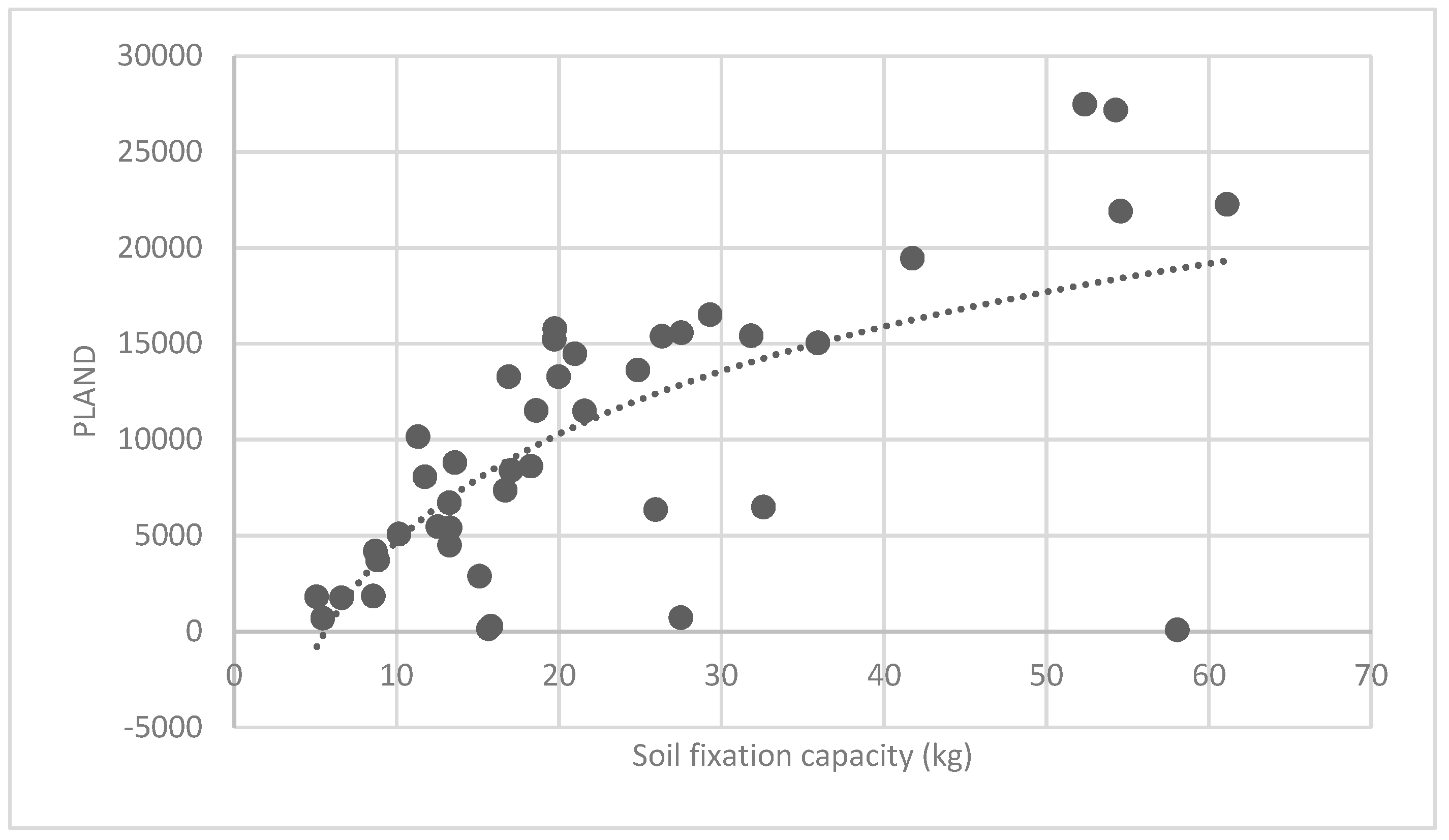
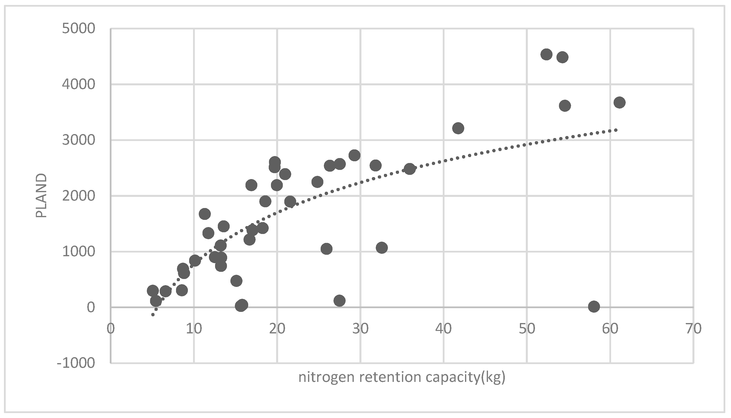
- The PLAND index of the forest land has a significant logarithmic relationship with the regulating service and supporting service in the analysis on association between the landscape pattern and ecosystem service quality. The critical PLAND index value is 30. When the PLAND value is smaller than 30, with growth of the proportion of the forest land, the quality of the regulating and supporting service will grow quickly. When the value is over 30, the quality growth will slow down. Additionally, the research results show that the shape index of the brush is exponentially associated with the quality of the ecosystem service, except in the Xishan area with most forest land in Haidian District (the quality of the ecosystem service of the forest land is dominant, and at this time it is not associated with the shape index of the brush spot). The critical LSI value is 50;
- (4)
- Finally, this paper proposes an area optimization strategy for green space in Haidian District, Beijing City, from the view of the ecosystem system service. The Xishan area is classified as the ecosystem red line to control city expansion. The regulating and supporting services can be enhanced in the northern flat area by improving the patch shape index. The ecosystem service capabilities can be improved by adding forest land in the existing green space for the southeastern urban areas.
Author Contributions
Funding
Acknowledgments
Conflicts of Interest
References
- Millennium Ecosystem Assessment. Ecosystem and Human Well-Being: A Framework for Assessment; Island Press: Washington, DC, USA, 2003. [Google Scholar]
- Che, S.; Wang, H. A summary of study on urban green space. J. Shanghai Jiaotong Univ. (Agric. Sci.) 2001, 3, 229–234. [Google Scholar]
- Mao, Q.Z.; Luo, S.H.; Ma, K.M.; Wu, J.G.; Tang, R.L.; Zhang, Y.X.; Le, B.; Zhang, T. Research advances in ecological assessment of urban green space. Acta Ecol. Sin. 2012, 32, 5589–5600. [Google Scholar]
- Li, F.; Wang, R. Research advance in ecosystem service of urban green space. Chin. J. Appl. Ecol. 2004, 15, 527–531. [Google Scholar]
- Liu, J.; Tian, Y.; Zhang, L. Study on the Relation of Urban Green Space Area and Ecological Response in Beijing City, China. In Conference on Environmental Pollution and Public Health; Scientific Research Publishing: Wuhan, China, 2010. [Google Scholar]
- Simonich, S.L.; Hites, R.A. Importance of vegetation in removing polycyclic aromatic hydrocarbons from the atmosphere. Nature 1994, 370, 49–51. [Google Scholar] [CrossRef]
- Beckett, K.P.; Freersmith, P.H.; Taylor, G. Urban woodlands: Their role in reducing the effects of particulate pollution. Environ. Pollut. 1998, 99, 347–360. [Google Scholar] [CrossRef]
- Bealey, W.J.; Mcdonald, A.G.; Nemitz, E.; Donovan, R.; Dragosits, U.; Duffy, T.R.; Fowler, D. Estimating the reduction of urban PM10 concentrations by trees within an environmental information system for planners. J. Environ. Manag. 2007, 85, 44–58. [Google Scholar] [CrossRef]
- Gratani, L.; Crescente, M.F.; Varone, L. Long-term monitoring of metal pollution by urban trees. Atmos. Environ. 2015, 42, 8273–8277. [Google Scholar] [CrossRef]
- Loram, A.; Tratalos, J.; Warren, P.H.; Gaston, K.J. Urban domestic gardens (X): The extent & structure of the resource in five major cities. Landsc. Ecol. 2007, 22, 601–615. [Google Scholar]
- Fujita, A.; Maeto, K.; Kagawa, Y.; Ito, N. Effects of forest fragmentation on species richness and composition of ground beetles (Coleoptera: Carabidae and Brachinidae) in urban landscapes. Entomol. Sci. 2010, 11, 39–48. [Google Scholar] [CrossRef]
- Carrete, M.; Tella, J.L.; Blanco, G.; Bertellotti, M. Effects of habitat degradation on the abundance, richness and diversity of raptors across Neotropical biomes. Boil. Conserv. 2009, 142, 2002–2011. [Google Scholar] [CrossRef]
- Zhou, Z.; Shao, T.; Wang, P.; Gao, C.; Xu, Y.; Guo, E.; Xu, L.; Ye, Z.; Peng, X.; Yu, C. The Spatial Structures and the Dust Retention Effects of Green-land Types in the Workshop District of Wuhan Iron and Steel Com-pany. Acta Ecol. Sin. 2002, 22, 2036–2040. [Google Scholar]
- Liu, Y.; Guo, J. The Research of NDVI-based Urban Green Space Landscape Pattern and Thermal Environment. Prog. Geogr. 2009, 28, 798–804. [Google Scholar]
- Shao, T.; Zhou, Z.; Wang, P.; Tang, W.; Liu, X.; Hu, X. Relationship between urban green-land landscape patterns and air pollution in the central district of Yichangcity. Chin. J. Appl. Ecol. 2004, 15, 691–696. [Google Scholar]
- Feng, L.; Wang, R. Evaluation, planning and prediction of ecosystem services of urban green space: A case study of Yangzhou City. Acta Ecol. Sin. 2003, 23, 1929–1936. [Google Scholar]
- Li, F.; Wang, R.S. Method and Practice for Ecological Planning of Urban Green Space—Yangzhou City as the Case Study. Urban Environ. Urban Ecol. 2003, 16, 46–48. [Google Scholar]
- Iverson, L.R.; Cook, E.A. Urban forest cover of the Chicago region and its relation to household density and income. Urban Ecosyst. 2000, 4, 105–124. [Google Scholar] [CrossRef]
- Burgman, M.A.; Keith, D.; Hopper, S.D.; Widyatmoko, D.; Drill, C. Threat syndromes and conservation of the Australian flora. Boil. Conserv. 2007, 134, 73–82. [Google Scholar] [CrossRef]
- Palmer, G.C.; Fitzsimons, J.A.; Antos, M.J.; White, J.G. Determinants of native avian richness in suburban remnant vegetation: Implications for conservation planning. Boil. Conserv. 2008, 141, 2329–2341. [Google Scholar] [CrossRef]
- Costanza, R.; D’Arge, R.; Groot, R.D.; Farber, S.; Grasso, M.; Hannon, B.; Limburg, K.; Naeem, S.; O’neill, R.V.; Paruelo, J.; et al. The value of the world’s ecosystem services and natural capital 1. Nature 1997, 387, 253–260. [Google Scholar] [CrossRef]
- Pimentel, D.; Wilson, C.; Mccullum, C.; Huang, R.; Dwen, P.; Flack, J.; Tran, Q.; Saltman, T.; Cliff, B. Economic and Environmental Benefits of Biodiversity. Bioscience 1997, 47, 747–757. [Google Scholar] [CrossRef] [Green Version]
- Sutton, P.C.; Costanza, R. Global estimates of market and non-market values derived from nighttime satellite imagery, land cover, and ecosystem service valuation. Ecol. Econ. 2002, 41, 509–527. [Google Scholar] [CrossRef]
- Reid, W.V.; Mooney, H.A.; Cropper, A.; Capistrano, D.; Carpenter, S.R.; Chopra, K.; Dasgupta, P.; Dietz, T.; Duraiappah, A.K.; Hassan, R.; et al. Millennium Ecosystem Assessment Synthesis Report. In Millennium Ecosystem Assessment; World Resources Institute: Washington, DC, USA, 2005. [Google Scholar]
- Gren, I.M.; Groth, K.H.; Sylvén, M. Economic Values of Danube Floodplains. J. Environ. Manag. 1995, 45, 333–345. [Google Scholar] [CrossRef]
- Dixon, J.A. Analysis and Management of Watersheds. In The Environment and Emerging Development Issues: Volume 2; Oxford Scholarship Online: Oxford, UK, 2000. [Google Scholar]
- Pattanayak, S.K. Valuing watershed services: Concepts and empirics from southeast Asia. Agric. Ecosyst. Environ. 2004, 104, 171–184. [Google Scholar] [CrossRef]
- Turner, R.K.; van den Bergh, J.C.J.M.; Söderqvist, T.; Barendregt, A.; Van Der Straaten, J.; Maltby, E.; Van Ierland, E.C. Ecological-economic analysis of wetlands: Scientific integration for management and policy. Ecol. Econ. 2000, 35, 7–23. [Google Scholar] [CrossRef]
- Hanley, N.D.; Ruffell, R.J. The contingent valuation of forest characteristics: Two experiments. J. Agric. Econ. 1993, 44, 218–229. [Google Scholar] [CrossRef]
- Loomis, J.; Kent, P.; Strange, L.; Fausch, K.; Covich, A. Measuring the total economic value of restoring ecosystem services in an impaired river basin: Results from a contingent valuation survey. Ecol. Econ. 2000, 33, 103–117. [Google Scholar] [CrossRef]
- Lal, P. Economic valuation of mangroves and decision-making in the Pacific. Ocean Coast. Manag. 2003, 46, 823–844. [Google Scholar] [CrossRef]
- Jakobsson, K.; Dragun, A.K. Contingent Valuation and Endangered Species: Methodological Issues and Applications; Edward Elgar Publishing: Cheltenham, UK, 1996. [Google Scholar]
- De Mendonça, M.J.; Sachsida, A.; Loureiro, P.R. A study on the valuing of biodiversity: The case of three endangered species in Brazil. Ecol. Econ. 2003, 46, 9–18. [Google Scholar] [CrossRef]
- Bandara, R.; Tisdell, C. The net benefit of saving the Asian elephant: A policy and contingent valuation study. Ecol. Econ. 2003, 48, 93–107. [Google Scholar] [CrossRef]
- Wu, L.; Lu, J.; Tong, C.; Liu, C. Valuation of wetland ecosystem services in the Yangtze River estuary. Resour. Environ. Yangtze Basin 2003, 12, 411–416. [Google Scholar]
- Xin, K.; Xiao, D. Wetland Ecosystem Service Valuation—A Case Researches on Panjin Area. Acta Ecol. Sin. 2002, 22, 1345–1349. [Google Scholar]
- Xiao, Y.; Xie, G.; An, K. Economic value of ecosystem services in Mangcuo Lake drainage basin. J. Appl. Ecol. 2003, 14, 676–680. [Google Scholar]
- Qiao, X. Assessment on urban ecosystem services of guangzhou city. J. Beijing Norm. Univ. 2003, 2, 268–272. [Google Scholar]
- Yang, Q.; Lan, C.; Xin, K. Evaluation on the value of the ecosystem services of the coastal zone in Guangdong and Hainan. Mar. Environ. Sci. 2003, 22, 25–29. [Google Scholar]
- Yu, X.; Xie, G.; Kai, A. The function and economic value of soil conservation of ecosystems in Qinghai-Tibet Plateau. Acta Ecol. Sin. 2003, 23, 2367–2378. [Google Scholar]
- Ouyang, Z.Y.; Wang, R.S. Ecosystem services and their economic valuation. Chin. J. Appl. Ecol. 1999, 5, 635–640. [Google Scholar]
- Ouyang, Z.; Wang, X.; Miao, H. A primary study on Chinese terrestrial ecosystem services and their ecological-economic values. Acta Ecol. Sin. 1999, 19, 607–613. [Google Scholar]
- Chen, Z.X.; Zhang, X.S. The value of ecosystem benefits in China. Chin. Sci. Bull. 2000, 45, 17–22. [Google Scholar] [CrossRef]
- He, H.; Yang, M.; Pan, Y.; Zhu, W. Measurement of terrestrial ecosystem service value in China based on remote sensing. Chin. J. Appl. Ecol. 2005, 16, 1122. [Google Scholar]
- Bi, X.L.; Ge, J.P. Evaluating Ecosystem Service Valuation in China Based on the IGBP Land Cover Datasets. J. Mt. Res. 2004, 22, 48–53. [Google Scholar]
- Xie, G.; Zhang, Y.; Lu, C.; Zheng, D.; Cheng, S. Study on valuation of rangeland ecosystem services of China. J. Nat. Resour. 2001, 16, 47–53. [Google Scholar]
- Xie, G.D.; Lu, C.X.; Leng, Y.F.; Zheng, D.U.; Li, S.C. Ecological assets valuation of the Tibetan Plateau. J. Natl. Resourc. 2003, 18, 189–196. [Google Scholar]
- Lu, C.; Xie, G.; Xiao, Y.; Yu, Y. Ecosystem diversity and economic valuation of Qinghai-Tibet Plateau. Acta Ecol. Sin. 2004, 24, 2749–2755. [Google Scholar]
- Burley, J.B. Multi-model habitat suitability index analysis in the Red River Valley. Landsc. Urban Plan. 1989, 17, 261–280. [Google Scholar] [CrossRef]
- Burley, J.B. A vegetation productivity equation for reclaiming surface mines in Clay County, Minnesota. Int. J. Surf. Min. Reclam. Environ. 1991, 5, 1–6. [Google Scholar] [CrossRef]
- Loures, L.; Loures, A.; Nunes, J.; Panagopoulos, T. The Green Revolution- converting post- industrial sites into urban parks—A case study analysis. Int. J. Surf. Min. Reclam. Environ. 2015, 9, 262–266. [Google Scholar]
- Cui, C.; Xu, X. Relative Assessment of Green Space Ecosystem Service in Beijing Region. Acta Sci. Nat. Univ. Pekin. 2010, 46, 271–278. [Google Scholar]
- Feng, T. Study on Agricultural Land Layout in Beijing Plain Area for Eco-friendly Target. Ph.D. Thesis, China Agricultural University, Beijing, China, 2016. [Google Scholar]
- Zhu, W.; Pan, Y.; Zhang, J. Estimation of net primary productivity of Chinese terrestrial vegetation based on remote sensing. J. Plant Ecol. 2007, 31, 413–424. [Google Scholar]
- Chen, Z.; Su, X.; Liu, S.; Zhang, X. Study on Ecological Efficiency of Urban Landscape Architecture in Beijing (3). Chin. Landsc. Archit. 1998, 3, 51–54. [Google Scholar]
- National Environmental Protection Agency. China’s Biodiversity: Country Study; China Environmental Press: Beijing, China, 1998.
- Yang, L. Studies on Water Consumption and Irrigation Model of Compound Plant Ecosystem in Urban Green Space in Beijing. Ph.D. Thesis, Beijing Forestry University, Beijing, China, 2012. [Google Scholar]
- Cheng, K.; Cui, G.; Wang, J.; Li, J. Evaluation on the economic value of the forest biodiversity in Labagoumen forest region. J. Beijing For. Univ. 2000, 22, 66–71. [Google Scholar]
- Wu, W. Study on the Value Assessment of Urban Green Space Ecosystem Services in Hangzhou. Ph.D. Thesis, Nanjing Forestry University, Nanjing, China, 2011. [Google Scholar]
- Wang, X. The String Studies of North Beijing Suburb Forest Park Based on Spatial Data Analysis. Ph.D. Thesis, Beijing Forestry University, Beijing, China, 2015. [Google Scholar]
- Luo, Z. Towards Landmark Recognition Via Large Scale Social Mesdia Mining. Master’s Thesis, South China University of Technology, Guangzhou, China, 2011. [Google Scholar]
- Xue, Y. Strategy for Propagation of Tourism Destination Image in Picture-Sharing Networks—Taking Flickr for Example. Master’s Thesis, University of Electronic Science and Technology of China, Chengdu, China, 2013. [Google Scholar]
- Cen, X. Correlation Analysis and Optimization between Land Use Landscape Patterns and Ecosystem Service Values—A Case Study of South Coast of Hangzhou Bay. Ph.D. Thesis, Zhejiang University, Hangzhou, China, 2016. [Google Scholar]
- Fragstats Help. Available online: http://222.28.119.57/cache/6/03/www.umass.edu/89aacb17a169768ca68ee14d9fcdbd93/fragstats.help.4.2.pdf (accessed on 2 April 2019).
- Tang, Y.; Shao, Q.; Cao, W.; Yang, F.; Liu, L.; Wu, D.; Zhou, S. The Ecosystem Services and Its Spatial Variation at Countyscale in the Southern Guizhou Based on Physical Assessment Method. Sci. Geogr. Sin.-CA 2018, 38, 122–134. [Google Scholar]
- Zhang, M.Y.; Wang, K.L.; Chen, H.S.; Zhang, C.H.; Liu, H.Y.; Yue, Y.M.; Fan, F.D. Quantified evaluation and analysis of ecosystem services in Karst areas based on remote sensing. Acta Ecol. Sin. 2009, 29, 5891–5901. [Google Scholar]


| Type of Land Coverage | Determination Mark | Picture |
|---|---|---|
| Forest land | Located in mountainous areas. The image is deep red, grainy, and has even texture. |  |
| Brush | Mainly located at the foot of hills and inside the city. This image includes deep red and shiny red and is grainy. |  |
| Grasslands | Its area is small inside the city. The image is shiny red. |  |
| Construction land | Distributed in the constructed urban area. The image is cyan and has distinctive geometric features. |  |
| Water area | The image is deep cyan and has a distinctive boundary and fine texture. |  |
| Other lands | Mainly located outside the city. The image is light gray and white. |  |
| Land Use and Land Cover Type | Regulating Service | Supporting Service | Cultural Service | |||||||||||
|---|---|---|---|---|---|---|---|---|---|---|---|---|---|---|
| Carbon Fixation And Oxygen Release | Cooling and Humidifying | Air Purification | Water Conservation | Soil Fixation Capacity | Fertility Conservation Capacity | Landscape Quality | ||||||||
| Carbon Fixation Capacity(Kg) | Oxygen Release Capacity (Kg) | Cooling Capacity (Kj) | Humidifying Capacity (Kg) | Sulfur-Dioxide Abstraction Capacity (Kg) | Oxynitride Absorption Capacity (Kg) | Hydrogen-Fluoride Absorption Capacity (Kg) | Dust Capacity (Kg) | Regulation Water Capacity (Kg) | Solid Fixation Capacity (Kg) | Nitrogen Capacity (Kg) | Phosphorous Retention Capacity (Kg) | Kalium Retention Capacity (Kg) | Photo Number | |
| Non-utilized land | 0.00 | 0.00 | 0.00 | 0.00 | 0.00 | 0.00 | 0.00 | 0.00 | 0.00 | 28,579.58 | 4715.63 | 371.53 | 4115.46 | 177 |
| Brush | 19,180.28 | 51, 348.66 | 200,744,800.46 | 18,981,221.98 | 374,230.23 | 29,521.19 | 6347.05 | 53,285,740.10 | 4,317,473.40 | 125,858.65 | 20,766.68 | 1636.16 | 18,123.65 | 297 |
| Construction | 0.00 | 0.00 | 0.00 | 0.00 | 0.00 | 0.00 | 0.00 | 0.00 | 0.00 | 0.00 | 0.00 | 0.00 | 0.00 | 847 |
| Forest land | 56,440.90 | 151,101.28 | 785,246,088.49 | 320,154,576.94 | 1,815,492.32 | 71,602.93 | 30,789.26 | 258,605,919.41 | 4,537,835.76 | 347,632.23 | 57,359.32 | 4519.22 | 50,059.04 | 1007 |
| Grassland | 14,346.55 | 38,408.01 | 13,111,226.57 | 53,592,790.68 | 178,667.05 | 28,188.33 | 3053.74 | 1,310,757.48 | 5,689,110.28 | 112,659.37 | 18,588.80 | 1464.57 | 16,222.95 | 459 |
| Water area | 2371.38 | 6348.56 | 61,303,263.82 | 24,990,252.41 | 0.00 | 0.00 | 0.00 | 0.00 | 0.00 | 0.00 | 0.00 | 0.00 | 0.00 | 576 |
| UNIT | Regulating Service | Supporting Service | Cultural Services | |||||||||||
|---|---|---|---|---|---|---|---|---|---|---|---|---|---|---|
| Carbon Fixation and Oxygen Release | Cooling and Humidifying | Air Purification | Water Conservation | Soil Capacity | Fertility Retention Capacity | Landscape Quality | ||||||||
| Carbon Fixation Capacity (kg) | Oxygen Release Capacity (kg) | Cooling Capacity (kJ) | Humidifying Capacity (kg) | Sulfur Dioxide Absorption Capacity (kg) | Oxynitride Absorption Capacity (kg) | Hydrogen Fluoride Absorption Capacity(kg) | Stagnant Dust capacity (kg) | Regulation Water Capacity (kg) | Soil Fixation Capacity (kg) | Nitrogen Retention Capacity (kg) | Phosphorous Retention Capacity (kg) | Potassium Retention Capacity (kg) | Photo Number | |
| Z01 | 98.86 | 264.66 | 1,089,370.95 | 278,651.71 | 2029.42 | 155.75 | 34.46 | 246,952.66 | 23,114.25 | 680.81 | 112.33 | 8.85 | 98.04 | 0.00 |
| Z02 | 644.02 | 1724.16 | 824,5341.47 | 2,965,043.41 | 17,843.74 | 893.99 | 302.73 | 2,430,765.79 | 90,016.27 | 4488.63 | 740.62 | 58.35 | 646.36 | 0.00 |
| Z03 | 1358.69 | 3637.43 | 18,922,395.65 | 7,166,506.47 | 34,361.95 | 1738.63 | 583.04 | 4,603,731.79 | 178,531.66 | 8609.15 | 1420.51 | 111.92 | 1239.72 | 0.04 |
| Z04 | 110.22 | 295.09 | 1,536,790.67 | 584,776.61 | 2776.80 | 141.09 | 47.12 | 370,682.43 | 14,584.04 | 711.59 | 117.41 | 9.25 | 102.47 | 0.00 |
| Z05 | 992.03 | 2655.82 | 11,897,912.59 | 3,614,960.46 | 23,155.86 | 1457.70 | 393.00 | 3,007,780.79 | 187,409.15 | 8046.84 | 1327.73 | 104.61 | 1158.74 | 0.00 |
| Z06 | 1754.57 | 4697.27 | 20,826,206.51 | 6,617,409.13 | 42,285.39 | 2,618.30 | 717.71 | 5,439,770.40 | 333,108.04 | 13,271.60 | 2189.81 | 172.53 | 1911.11 | 0.01 |
| Z07 | 1159.69 | 3104.67 | 15,638,070.60 | 5,872,025.54 | 31,094.95 | 1,533.76 | 527.56 | 4,213,242.78 | 151,712.59 | 7350.16 | 1212.78 | 95.55 | 1058.42 | 0.05 |
| Z08 | 272.68 | 730.01 | 3,598,599.99 | 1,349,254.21 | 7883.77 | 366.89 | 133.73 | 1,090,693.73 | 33,058.13 | 1791.80 | 295.65 | 23.29 | 258.02 | 0.04 |
| Z09 | 1017.61 | 2724.30 | 13,620,410.84 | 5,280,237.49 | 30,637.44 | 1350.17 | 519.67 | 4,275,282.07 | 110,540.70 | 6471.18 | 1067.74 | 84.13 | 931.85 | 0.02 |
| Z10 | 2444.64 | 6544.69 | 30,499,332.87 | 9,836,865.91 | 64,361.80 | 3435.97 | 1091.86 | 8,838,893.85 | 371,932.04 | 16,506.10 | 2723.51 | 214.58 | 2376.88 | 0.03 |
| Z11 | 2475.51 | 6627.34 | 33,885,723.79 | 11,622,445.09 | 49,558.04 | 3234.71 | 841.34 | 6,184,853.58 | 431,598.88 | 15,769.13 | 2601.91 | 205.00 | 2270.75 | 0.33 |
| Z12 | 1254.29 | 3357.93 | 16,053,160.64 | 6,044,347.02 | 32,990.58 | 1770.74 | 559.89 | 4,297,271.60 | 196,687.32 | 8380.05 | 1382.71 | 108.94 | 1206.73 | 0.11 |
| Z13 | 825.73 | 2210.62 | 10,820,779.16 | 4,072,016.48 | 23,927.26 | 1121.23 | 405.90 | 3,296,572.88 | 102,326.90 | 5388.33 | 889.07 | 70.05 | 775.92 | 0.07 |
| Z14 | 39.03 | 104.48 | 508,925.66 | 190,532.11 | 1122.65 | 53.28 | 19.04 | 154,174.32 | 4964.20 | 255.04 | 42.08 | 3.32 | 36.73 | 0.00 |
| Z15 | 11.04 | 29.54 | 153,276.89 | 62,293.31 | 354.00 | 14.02 | 6.00 | 50,406.92 | 899.46 | 68.01 | 11.22 | 0.88 | 9.79 | 0.00 |
| Z16 | 4306.32 | 11,528.72 | 58,485,294.22 | 23,067,885.31 | 132,947.67 | 5616.88 | 2254.90 | 18,719,387.88 | 421,461.26 | 27,470.03 | 4532.56 | 357.11 | 3955.68 | 0.01 |
| Z17 | 3445.06 | 9222.98 | 45,908,339.00 | 17,463,742.11 | 102,528.69 | 4580.14 | 1739.08 | 14,327,857.48 | 383,735.16 | 22,249.93 | 3671.24 | 289.25 | 3203.99 | 0.11 |
| Z18 | 2413.15 | 6460.37 | 33,359,198.32 | 12,620,545.62 | 63,591.12 | 3102.81 | 1078.87 | 8,641,584.33 | 302,093.20 | 15,027.10 | 2479.47 | 195.35 | 2163.90 | 0.76 |
| Z19 | 1804.30 | 4830.40 | 23,652,766.43 | 8,782,159.02 | 43,000.84 | 2495.35 | 729.93 | 5,443,177.37 | 301,894.22 | 11,478.61 | 1893.97 | 149.22 | 1652.92 | 0.28 |
| Z20 | 841.79 | 2253.59 | 11,003,446.57 | 4,048,156.36 | 22,226.48 | 1152.85 | 377.14 | 2,967,955.60 | 122,113.09 | 5451.04 | 899.42 | 70.86 | 784.95 | 0.03 |
| Z21 | 4174.34 | 11,175.37 | 53,256,159.48 | 20,560,698.51 | 114,850.11 | 5919.35 | 1949.03 | 15,081,816.33 | 626,560.01 | 27,167.69 | 4482.67 | 353.18 | 3912.15 | 0.00 |
| Z22 | 2976.66 | 7968.99 | 38,109,493.67 | 14,086,158.38 | 82,469.26 | 4158.21 | 1399.25 | 11,102,007.08 | 424,272.57 | 19,447.45 | 3208.83 | 252.82 | 2800.43 | 0.04 |
| Z23 | 2280.10 | 6104.20 | 29,261,291.47 | 10,377,309.17 | 60,981.91 | 3159.30 | 1034.65 | 8,241,275.62 | 332,561.04 | 15,404.64 | 2541.76 | 200.26 | 2218.27 | 0.00 |
| Z24 | 2065.43 | 5529.48 | 25,808,837.66 | 8,838,491.05 | 52,043.29 | 2946.78 | 883.18 | 6,843,307.78 | 344,357.89 | 13,618.26 | 2247.01 | 177.04 | 1961.03 | 0.01 |
| Z25 | 1720.27 | 4605.44 | 20,862,880.06 | 7,039,270.69 | 41,665.70 | 2537.09 | 707.24 | 5,307,363.69 | 319,282.49 | 11,508.88 | 1898.96 | 149.62 | 1657.28 | 0.01 |
| Z26 | 1252.72 | 3353.72 | 14,941,163.10 | 5,259,749.86 | 30,006.27 | 1896.38 | 509.47 | 3,683,063.26 | 248,102.26 | 8790.34 | 1450.41 | 114.27 | 1265.81 | 0.05 |
| Z27 | 772.21 | 2067.34 | 9,685,283.47 | 3,462,063.18 | 20,035.40 | 1103.73 | 340.01 | 2,626,304.53 | 125,670.01 | 5070.79 | 836.68 | 65.92 | 730.19 | 0.02 |
| Z28 | 277.14 | 741.94 | 3,553,896.42 | 1,274,534.50 | 5756.73 | 395.03 | 97.77 | 674,924.88 | 55,272.85 | 1738.43 | 286.84 | 22.60 | 250.33 | 0.00 |
| Z29 | 3409.75 | 9128.46 | 44,331,653.58 | 16,005,657.53 | 97,783.56 | 4633.20 | 1658.67 | 13,595,988.24 | 427,829.40 | 21,897.90 | 3613.15 | 284.67 | 3153.30 | 0.01 |
| Z30 | 2,289.91 | 6130.46 | 28,221,265.28 | 9,338,148.84 | 57,401.49 | 3296.12 | 974.08 | 7,578,555.21 | 389,831.71 | 15,374.35 | 2536.77 | 199.87 | 2213.91 | 0.02 |
| Z31 | 2368.65 | 6341.25 | 30,554,575.51 | 10,733,548.30 | 57,400.27 | 3290.20 | 974.17 | 7, 466, 149.98 | 390,339.76 | 15,562.46 | 2567.81 | 202.31 | 2240.99 | 0.02 |
| Z32 | 2120.60 | 5677.19 | 25,508,689.05 | 9,026,399.78 | 46,906.70 | 3209.01 | 796.67 | 5,497,912.02 | 448,152.65 | 15,221.63 | 2511.57 | 197.88 | 2191.91 | 0.01 |
| Z33 | 1336.63 | 3578.38 | 15,598,446.89 | 4,830,956.52 | 30,344.56 | 2031.25 | 515.16 | 3,779,051.51 | 275,999.23 | 10,140.76 | 1673.23 | 131.83 | 1460.27 | 0.00 |
| Z34 | 259.69 | 695.23 | 2,799,377.97 | 929,508.65 | 5054.12 | 433.65 | 85.92 | 509,150.49 | 69,797.08 | 1841.38 | 303.83 | 23.94 | 265.16 | 0.00 |
| Z35 | 19.10 | 51.13 | 242,718.12 | 92,488.41 | 522.23 | 27.13 | 8.86 | 68,662.22 | 2896.77 | 132.29 | 21.83 | 1.72 | 19.05 | 0.00 |
| Z36 | 977.37 | 2616.57 | 11,846,800.72 | 3,551,967.99 | 24,814.14 | 1405.03 | 420.98 | 3,390,078.31 | 162,088.86 | 6340.20 | 1046.13 | 82.42 | 912.99 | 0.00 |
| Z37 | 965.42 | 2584.59 | 11,217,703.68 | 3,397,937.30 | 21,547.69 | 1470.35 | 365.82 | 2,675,715.17 | 202,521.02 | 6703.00 | 1106.00 | 87.14 | 965.23 | 0.02 |
| Z38 | 1967.22 | 5266.56 | 23,918,451.96 | 7,747,075.91 | 46,978.34 | 2875.38 | 797.35 | 6,061,153.49 | 362,107.99 | 13,273.25 | 2190.09 | 172.55 | 1911.35 | 0.00 |
| Z39 | 2203.63 | 5899.48 | 27,902,641.09 | 9,603,191.19 | 49,100.05 | 3138.55 | 833.59 | 6,096,387.62 | 412,946.76 | 14,460.32 | 2385.95 | 187.98 | 2082.29 | 0.01 |
| Z40 | 556.22 | 1489.08 | 7,005,562.57 | 2,433,737.50 | 12,312.70 | 798.94 | 209.06 | 1,509,276.71 | 106,601.53 | 3705.51 | 611.41 | 48.17 | 533.59 | 0.01 |
| Z41 | 427.42 | 1144.28 | 5,136,519.60 | 1,697,036.12 | 10,530.48 | 632.83 | 178.73 | 1,358,032.37 | 78,498.06 | 2865.72 | 472.84 | 37.25 | 412.66 | 0.00 |
| Z42 | 592.07 | 1585.06 | 6,872,312.66 | 2,192,461.65 | 13,598.89 | 907.99 | 230.89 | 1,675,970.81 | 123,450.50 | 4181.65 | 689.97 | 54.36 | 602.16 | 0.01 |
| AVG | 2144.59 | 5741.41 | 27,375,619.42 | 9,701,586.37 | 55,006.22 | 3003.30 | 933.42 | 7,274,175.82 | 337,796.45 | 14,277.20 | 2355.74 | 185.60 | 2055.92 | 0.08 |
| UNIT | TYPE | PLAND 1 | LSI 2 | IJI 3 |
|---|---|---|---|---|
| Z01 | Other land | 0.66 | 5.29 | 71.81 |
| Brush | 14.72 | 19.54 | 55.16 | |
| Construction land | 69.64 | 13.26 | 67.58 | |
| Forest land | 5.46 | 11.91 | 72.18 | |
| Grasslands | 9.33 | 15.17 | 61.22 | |
| Water area | 0.19 | 2.26 | 51.57 | |
| Z02 | Other land | 2.23 | 20.00 | 71.95 |
| Brush | 4.28 | 49.04 | 62.9 | |
| Construction land | 77.21 | 28.18 | 66.27 | |
| Forest land | 13.26 | 47.24 | 63.00 | |
| Grasslands | 2.96 | 37.35 | 69.16 | |
| Water area | 0.05 | 4.51 | 68.58 | |
| Z03 | Other land | 2.57 | 26.97 | 63.70 |
| Brush | 4.12 | 56.82 | 72.57 | |
| Construction land | 66.34 | 33.59 | 61.25 | |
| Forest land | 18.26 | 58.9 | 70.57 | |
| Grasslands | 5.43 | 50.63 | 73.34 | |
| Water area | 3.28 | 6.30 | 71.41 | |
| Z04 | Other land | 13.75 | 3.86 | 22.24 |
| Construction land | 58.75 | 2.21 | 65.34 | |
| Forest land | 27.50 | 14.11 | 57.18 | |
| Z05 | Other land | 9.20 | 32.51 | 62.00 |
| Brush | 12.68 | 55.30 | 70.40 | |
| Construction land | 58.28 | 37.07 | 75.19 | |
| Forest land | 11.75 | 39.18 | 78.09 | |
| Grasslands | 7.40 | 35.58 | 72.89 | |
| Water area | 0.68 | 4.41 | 63.95 | |
| Z06 | Other land | 7.00 | 33.61 | 83.14 |
| Brush | 14.07 | 75.63 | 80.46 | |
| Construction land | 51.07 | 37.20 | 78.86 | |
| Forest land | 16.91 | 61.30 | 81.70 | |
| Grasslands | 10.88 | 57.06 | 78.14 | |
| Water area | 0.08 | 4.52 | 57.40 | |
| Z07 | Other land | 1.11 | 19.08 | 62.11 |
| Brush | 3.78 | 55.73 | 66.61 | |
| Construction land | 72.90 | 28.59 | 51.11 | |
| Forest land | 16.70 | 62.65 | 60.50 | |
| Grasslands | 4.03 | 45.95 | 70.93 | |
| Water area | 1.49 | 8.39 | 69.60 | |
| Z08 | Other land | 0.47 | 8.92 | 81.27 |
| Brush | 1.02 | 28.35 | 62.46 | |
| Construction land | 92.67 | 15.67 | 56.01 | |
| Forest land | 5.08 | 34.65 | 48.47 | |
| Grasslands | 0.70 | 20.23 | 66.29 | |
| Water area | 0.05 | 5.78 | 58.57 | |
| Z09 | Other land | 0.63 | 12.90 | 70.82 |
| Brush | 3.73 | 27.61 | 64.29 | |
| Construction land | 60.03 | 19.32 | 75.67 | |
| Forest land | 32.58 | 12.67 | 67.81 | |
| Grasslands | 3.02 | 22.10 | 46.53 | |
| Water area | 0 | 1.22 | 37.76 | |
| Z10 | Other land | 3.69 | 35.47 | 64.50 |
| Brush | 19.51 | 71.07 | 65.47 | |
| Construction land | 41.04 | 41.86 | 62.22 | |
| Forest land | 29.31 | 39.20 | 68.13 | |
| Grasslands | 6.13 | 39.65 | 63.47 | |
| Water area | 0.34 | 5.53 | 66.49 | |
| Z11 | Other land | 6.78 | 42.92 | 76.93 |
| Brush | 17.16 | 76.23 | 73.49 | |
| Construction land | 29.15 | 46.22 | 74.22 | |
| Forest land | 19.74 | 59.23 | 77.81 | |
| Grasslands | 17.00 | 61.61 | 75.86 | |
| Water area | 10.16 | 7.61 | 64.43 | |
| Z12 | Other land | 1.37 | 17.36 | 68.83 |
| Brush | 3.76 | 52.12 | 75.55 | |
| Construction land | 69.71 | 27.17 | 56.17 | |
| Forest land | 17.04 | 60.77 | 66.76 | |
| Grasslands | 7.50 | 38.24 | 74.70 | |
| Water area | 0.61 | 7.24 | 71.63 | |
| Z13 | Other land | 0.64 | 13.10 | 54.00 |
| Brush | 2.55 | 46.25 | 61.54 | |
| Construction land | 81.42 | 22.31 | 46.99 | |
| Forest land | 13.30 | 51.07 | 48.23 | |
| Grasslands | 2.09 | 31.59 | 62.93 | |
| Water area | 0.01 | 3.53 | 44.49 | |
| Z14 | Other land | 0.73 | 2.83 | 77.26 |
| Brush | 3.26 | 9.80 | 65.93 | |
| Construction land | 77.45 | 6.17 | 78.75 | |
| Forest land | 15.82 | 8.90 | 69.48 | |
| Grasslands | 2.74 | 9.02 | 72.13 | |
| Z15 | Brush | 0.39 | 1.27 | 0 |
| Construction land | 41.48 | 3.78 | 49.97 | |
| Forest land | 58.07 | 1.46 | 70.58 | |
| Grasslands | 0.06 | 1.00 | 0 | |
| Z16 | Other land | 1.74 | 25.37 | 66.3 |
| Brush | 3.82 | 44.58 | 66.83 | |
| Construction land | 39.39 | 30.06 | 72.36 | |
| Forest land | 52.36 | 15.65 | 75.41 | |
| Grasslands | 2.67 | 27.77 | 43.62 | |
| Water area | 0.01 | 1.84 | 67.15 | |
| Z17 | Other land | 2.80 | 23.24 | 73.89 |
| Brush | 9.82 | 58.59 | 70.65 | |
| Construction land | 20.68 | 28.41 | 64.97 | |
| Forest land | 61.14 | 26.42 | 79.77 | |
| Grasslands | 5.38 | 36.42 | 56.66 | |
| Water area | 0.19 | 3.00 | 72.52 | |
| Z18 | Other land | 2.86 | 28.31 | 80.39 |
| Brush | 7.67 | 65.49 | 77.71 | |
| Construction land | 40.62 | 34.19 | 71.91 | |
| Forest land | 35.95 | 41.70 | 83.50 | |
| Grasslands | 8.10 | 47.45 | 82.63 | |
| Water area | 4.80 | 8.28 | 77.04 | |
| Z19 | Other land | 1.26 | 19.18 | 75.62 |
| Brush | 6.75 | 60.58 | 76.18 | |
| Construction land | 53.82 | 31.35 | 68.00 | |
| Forest land | 21.57 | 60.89 | 76.07 | |
| Grasslands | 13.27 | 49.66 | 75.18 | |
| Water area | 3.33 | 9.19 | 80.47 | |
| Z20 | Other land | 0.80 | 9.71 | 64.46 |
| Brush | 3.61 | 48.89 | 68.00 | |
| Construction land | 78.21 | 22.55 | 61.80 | |
| Forest land | 12.54 | 45.40 | 64.00 | |
| Grasslands | 4.05 | 36.16 | 68.03 | |
| Water area | 0.79 | 8.38 | 80.11 | |
| Z21 | Other land | 0.17 | 9.79 | 81.42 |
| Brush | 7.56 | 33.29 | 55.43 | |
| Construction land | 17.15 | 20.68 | 73.75 | |
| Forest land | 54.28 | 21.00 | 43.87 | |
| Grasslands | 20.85 | 31.27 | 38.91 | |
| Water area | 0 | 1.10 | 56.98 | |
| Z22 | Other land | 1.25 | 25.77 | 75.74 |
| Brush | 10.46 | 63.30 | 66.81 | |
| Construction land | 34.89 | 27.07 | 64.65 | |
| Forest land | 41.75 | 32.59 | 68.48 | |
| Grasslands | 11.54 | 43.28 | 58.92 | |
| Water area | 0.10 | 4.05 | 70.47 | |
| Z23 | Other land | 4.14 | 32.12 | 79.3 |
| Brush | 12.16 | 69.05 | 76.88 | |
| Construction land | 42.18 | 33.47 | 80.30 | |
| Forest land | 31.83 | 42.12 | 83.52 | |
| Grasslands | 8.65 | 42.55 | 76.83 | |
| Water area | 1.03 | 9.87 | 79.97 | |
| Z24 | Other land | 1.53 | 25.38 | 85.72 |
| Brush | 13.19 | 66.45 | 74.40 | |
| Construction land | 48.25 | 30.65 | 74.54 | |
| Forest land | 24.85 | 41.59 | 82.58 | |
| Grasslands | 11.09 | 47.94 | 75.34 | |
| Water area | 1.09 | 10.56 | 77.30 | |
| Z25 | Other land | 1.00 | 17.27 | 86.23 |
| Brush | 11.48 | 64.90 | 71.43 | |
| Construction land | 56.13 | 31.37 | 71.38 | |
| Forest land | 18.60 | 41.01 | 74.63 | |
| Grasslands | 12.21 | 40.58 | 73.43 | |
| Water area | 0.59 | 8.51 | 85.9 | |
| Z26 | Other land | 1.80 | 17.71 | 81.11 |
| Brush | 6.52 | 61.30 | 65.23 | |
| Construction land | 66.46 | 37.10 | 64.17 | |
| Forest land | 13.59 | 62.54 | 59.55 | |
| Grasslands | 11.50 | 45.05 | 67.74 | |
| Water area | 0.14 | 3.71 | 65.32 | |
| Z27 | Other land | 0.34 | 6.30 | 75.93 |
| Brush | 3.81 | 54.67 | 59.47 | |
| Construction land | 81.03 | 26.96 | 59.26 | |
| Forest land | 10.15 | 55.17 | 50.45 | |
| Grasslands | 4.43 | 34.36 | 65.64 | |
| Water area | 0.23 | 4.98 | 72.53 | |
| Z28 | Other land | 0.19 | 7.16 | 86.48 |
| Brush | 3.77 | 24.65 | 72.16 | |
| Construction land | 79.70 | 13.84 | 76.01 | |
| Forest land | 6.61 | 20.91 | 75.89 | |
| Grasslands | 7.79 | 17.07 | 74.05 | |
| Water area | 1.93 | 7.00 | 71.89 | |
| Z29 | Other land | 1.36 | 20.30 | 67.91 |
| Brush | 16.19 | 53.69 | 60.01 | |
| Construction land | 21.40 | 23.51 | 63.30 | |
| Forest land | 54.58 | 27.55 | 53.28 | |
| Grasslands | 6.46 | 42.68 | 47.44 | |
| Water area | 0.02 | 2.33 | 80.08 | |
| Z30 | Other land | 2.51 | 25.43 | 84.94 |
| Brush | 16.96 | 72.39 | 75.23 | |
| Construction land | 41.78 | 35.48 | 71.48 | |
| Forest land | 26.34 | 45.49 | 80.24 | |
| Grasslands | 11.61 | 47.93 | 73.9 | |
| Water area | 0.80 | 9.14 | 75.18 | |
| Z31 | Other land | 3.41 | 28.62 | 71.28 |
| Brush | 13.50 | 68.49 | 77.8 | |
| Construction land | 38.33 | 31.50 | 81.03 | |
| Forest land | 27.53 | 43.89 | 82.87 | |
| Grasslands | 13.81 | 49.84 | 76.46 | |
| Water area | 3.41 | 12.14 | 75.42 | |
| Z32 | Other land | 5.30 | 34.84 | 72.40 |
| Brush | 10.76 | 69.86 | 76.61 | |
| Construction land | 39.31 | 37.89 | 86.12 | |
| Forest land | 19.70 | 39.12 | 83.56 | |
| Grasslands | 23.02 | 41.24 | 81.32 | |
| Water area | 1.91 | 8.47 | 84.55 | |
| Z33 | Other land | 5.46 | 25.44 | 58.27 |
| Brush | 11.97 | 70.77 | 63.58 | |
| Construction land | 60.34 | 39.33 | 73.77 | |
| Forest land | 11.32 | 46.34 | 72.04 | |
| Grasslands | 10.56 | 44.27 | 66.33 | |
| Water area | 0.35 | 6.61 | 68.59 | |
| Z34 | Other land | 0.16 | 6.52 | 67.95 |
| Brush | 9.67 | 24.17 | 57.96 | |
| Construction land | 57.61 | 20.82 | 67.87 | |
| Forest land | 8.57 | 18.97 | 63.05 | |
| Grasslands | 23.93 | 21.21 | 62.07 | |
| Water area | 0.06 | 1.21 | 28.38 | |
| Z35 | Other land | 1.97 | 2.57 | 49.8 |
| Brush | 2.75 | 7.69 | 75.92 | |
| Construction land | 73.61 | 5.64 | 76.48 | |
| Forest land | 15.65 | 8.01 | 73.66 | |
| Grasslands | 6.01 | 6.57 | 75.51 | |
| Z36 | Other land | 0.20 | 3.70 | 66.07 |
| Brush | 24.45 | 39.98 | 62.19 | |
| Construction land | 42.54 | 26.83 | 40.74 | |
| Forest land | 25.95 | 24.15 | 45.84 | |
| Grasslands | 6.86 | 28.59 | 41.42 | |
| Water area | 0 | 1.17 | 59.21 | |
| Z37 | Other land | 2.17 | 20.84 | 76.08 |
| Brush | 15.93 | 49.91 | 66.16 | |
| Construction land | 54.85 | 30.59 | 69.00 | |
| Forest land | 13.24 | 35.47 | 75.19 | |
| Grasslands | 13.26 | 29.74 | 65.43 | |
| Water area | 0.56 | 7.03 | 64.31 | |
| Z38 | Other land | 2.20 | 27.43 | 64.59 |
| Brush | 15.70 | 60.88 | 68.76 | |
| Construction land | 48.82 | 32.75 | 70.69 | |
| Forest land | 19.98 | 36.58 | 68.70 | |
| Grasslands | 12.25 | 40.38 | 66.55 | |
| Water area | 1.05 | 6.22 | 51.72 | |
| Z39 | Other land | 2.69 | 32.62 | 66.24 |
| Brush | 13.87 | 72.93 | 69.52 | |
| Construction land | 41.05 | 35.94 | 76.67 | |
| Forest land | 20.97 | 46.04 | 72.48 | |
| Grasslands | 17.46 | 49.18 | 68.9 | |
| Water area | 3.96 | 9.21 | 76.52 | |
| Z40 | Other land | 1.39 | 12.51 | 69.89 |
| Brush | 5.56 | 37.99 | 72.20 | |
| Construction land | 74.58 | 19.45 | 80.23 | |
| Forest land | 8.83 | 22.16 | 77.36 | |
| Grasslands | 8.01 | 25.46 | 72.58 | |
| Water area | 1.63 | 6.32 | 89.73 | |
| Z41 | Other land | 0.66 | 12.48 | 74.28 |
| Brush | 10.04 | 27.95 | 69.13 | |
| Construction land | 65.21 | 14.03 | 74.91 | |
| Forest land | 15.11 | 16.46 | 64.00 | |
| Grasslands | 8.91 | 20.56 | 63.07 | |
| Water area | 0.07 | 2.63 | 66.01 | |
| Z42 | Other land | 1.47 | 17.66 | 72.36 |
| Brush | 7.85 | 39.63 | 71.74 | |
| Construction land | 73.56 | 19.24 | 75.59 | |
| Forest land | 8.70 | 24.93 | 72.80 | |
| Grasslands | 8.36 | 26.4 | 67.77 | |
| Water area | 0.05 | 3.81 | 62.56 |
© 2019 by the authors. Licensee MDPI, Basel, Switzerland. This article is an open access article distributed under the terms and conditions of the Creative Commons Attribution (CC BY) license (http://creativecommons.org/licenses/by/4.0/).
Share and Cite
Wang, B.; Liu, Z.; Mei, Y.; Li, W. Assessment of Ecosystem Service Quality and Its Correlation with Landscape Patterns in Haidian District, Beijing. Int. J. Environ. Res. Public Health 2019, 16, 1248. https://0-doi-org.brum.beds.ac.uk/10.3390/ijerph16071248
Wang B, Liu Z, Mei Y, Li W. Assessment of Ecosystem Service Quality and Its Correlation with Landscape Patterns in Haidian District, Beijing. International Journal of Environmental Research and Public Health. 2019; 16(7):1248. https://0-doi-org.brum.beds.ac.uk/10.3390/ijerph16071248
Chicago/Turabian StyleWang, Boya, Zhicheng Liu, Yuting Mei, and Wenjie Li. 2019. "Assessment of Ecosystem Service Quality and Its Correlation with Landscape Patterns in Haidian District, Beijing" International Journal of Environmental Research and Public Health 16, no. 7: 1248. https://0-doi-org.brum.beds.ac.uk/10.3390/ijerph16071248