Supervised Machine Learning Algorithms for Bioelectromagnetics: Prediction Models and Feature Selection Techniques Using Data from Weak Radiofrequency Radiation Effect on Human and Animals Cells


Abstract
:1. Introduction
1.1. Background
1.2. Motivation
- Extract data from 300 peer-reviewed scientific publications (1990–2015) describing 1127 experimental investigations in cell-based in vitro models (human and animal species).
- Identify the most suitable features or attributes to be utilized in prediction models to provide insight into key factors that determine the possible impact of RF-EMF in in-vitro studies while using domain knowledge, Principal Component Analysis (PCA), and Chi-squared feature selection techniques.
- Develop a grouping or clustering strategies to allocate these selected features into five different laboratory experiment scenarios. This will produce five different feature groups or distributions for each laboratory experiment.
- Develop a prediction model to observe the possible impact without performing in-vitro laboratory experiments. This is the first time that the supervised machine learning approach has been used for the characterization of weak RF-EMF exposure scenarios on human and animal cells.
- Compare each classifier’s prediction performance while using seven measures to obtain the decision on its suitability, while using the percentage of the model accuracy (PCC), Root Mean Squared Error (RMSE), precision, sensitivity (recall), 1 − specificity, Area under the ROC Curve (AUC), and precision-recall (PRC Area) for each classification method.
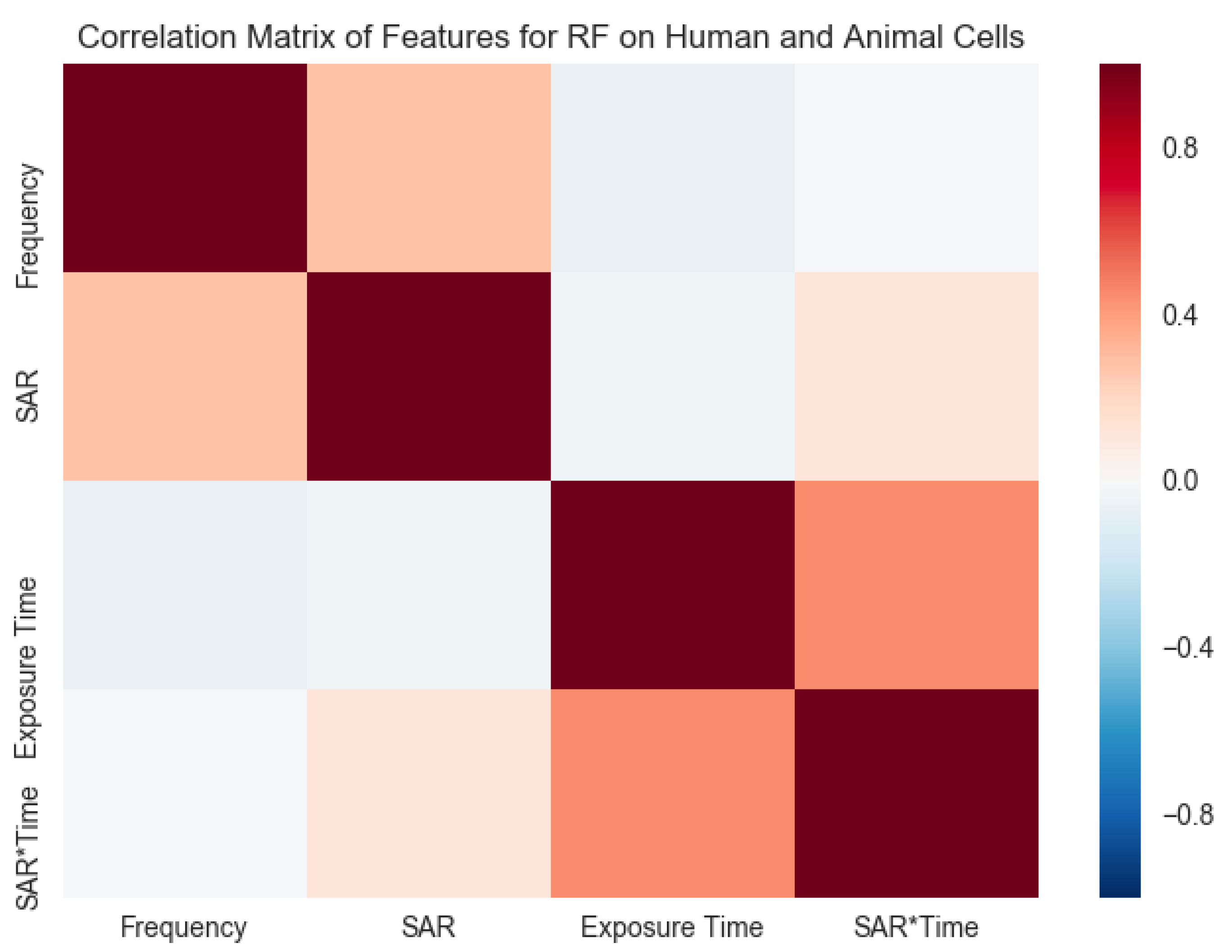
- Identify a robust correlation between exposure time with SAR×time (impact of accumulated SAR within the exposure period) and SAR with the frequency of weak RF-EMF on human and animal species. In contrast, the relationship between frequency and exposure time was not significant.
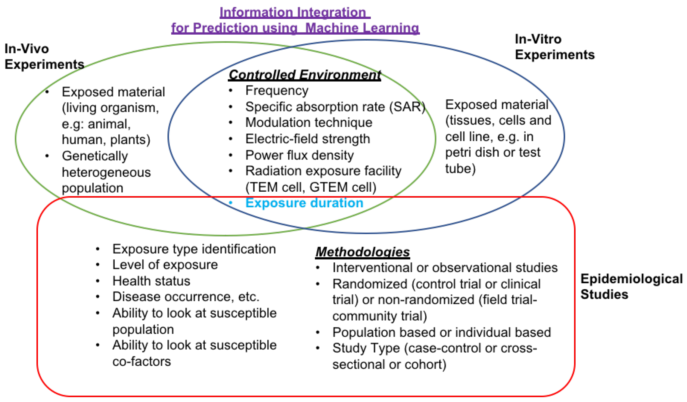
2. Materials and Methods
2.1. Feature Selection Methods for Classification
2.1.1. Principal Component Analysis (PCA)
2.1.2. Chi-Squared Feature Selection ()
2.2. Supervised Machine Learning
2.3. Data Collection
2.4. Data Pre-Processing and Inclusion Criteria
2.5. Data Analysis
2.6. Evaluation Measures of Binary Classifiers
3. Results
3.1. Feature Selection Methods for Classification
3.2. Prediction Using Supervised Machine Learning
4. Discussion
5. Future Directions
5.1. Data, Data Size, Data Quality, Parallel, and Distributed Computing Challenges
5.2. Feature Selection Strategy
5.3. Machine Learning, Deep Learning, and Artificial Intelligence for Future Bioelectromagnetics
6. Conclusions
Funding
Conflicts of Interest
Appendix A

| Algorithm/Classifier Name | Classifier Type | Description | Capabilities (Features/Attributes Allowed by the Algorithm) | Citation |
|---|---|---|---|---|
| K-nearest neighbours’ classifier (kNN) | Lazy | The appropriate value of K, based on cross-validation, can be selected. The kNN (k-number of neighbours) uses the nearest neighbour search algorithm. Using cross-validation, the algorithm chooses the best k value between 1 and the value mentioned as the kNN parameter | Numeric, nominal, binary, date, unary, missing values | Aha (1991) [82] |
| Random Forest | Trees | Random forests algorithm builds a forest of random trees. This considers a mixture of tree predictors (where each tree depends on the independent values of a random vector sampled) and employs similar distribution for all trees in the forest. When various trees in the forest become huge, the generalization error for forests converges as far as possible to a limit. The error of the forest tree classifiers relies upon the power of the individual trees and the correlation between the trees. In this method, the data does not require to be re-scaled or transformed. Primarily, Random forest tackles outliers by binning them | Numeric, nominal, binary, date, unary, missing values | Breiman (2001) [83] |
| Bagging | Meta | A Bagging classifier is a meta-estimator that provides base classifiers with each on random subsets of the original dataset. Then it aggregates the prediction to form a final prediction. Such a meta-estimator can be used to reduce the variance of a black-box estimator (e.g., a decision tree) by introducing randomization into its construction procedure | Numeric, nominal, binary, date, unary, missing values | Breiman (1996) [84] |
| J48 | Trees | The J48 is a classification algorithm which generates a decision tree which produces a pruned or unpruned C4.5 decision tree. A number of folds decide the volume of data used for reduced-error pruning. One-fold is utilized for pruning, and the rest is for growing the tree | Numeric, nominal, binary, date, unary, missing values | Quinlan (1993) [85] |
| Support-vector machines (SVM, Linear Kernel) | Function | The SVM classifier globally substitutes all missing values. This also transforms nominal attributes into binary values. Then, by default, it normalizes all attributes. Hence, the coefficients in the output are based on the normalized data, not the original data, which is essential for interpreting the classifier. To achieve probability estimates, use the option that provides the logistic regression method to the outputs of the support vector machine | Numeric, nominal, binary, unary, missing values | Platt (1998) [86]. |
| Jrip | Rules | The JRip class implements a propositional rule learner called Repeated Incremental Pruning to Produce Error Reduction (RIPPER). It is established in association rules with reduced error pruning (REP), a popular and efficient method seen in decision tree algorithms. The algorithm operates through a few phases: initialization, building stage, grow phase, prune phase, optimization and selection stage | Numeric, nominal, binary, date, unary, missing values | Cohen (1995) [87] |
| Decision Table | Rules | The Decision Table is a class for building and utilizing an easy decision table in the classifier. It also is represented as a programming language or as in decision trees as a series of if-then-else and switch-case statements. The learning decision tables comprises choosing the correct attributes to be incorporated. A decision table is seen as balanced if it includes each conceivable mixture of input variables | Numeric, nominal, binary, date, unary, missing values | Kohavi (1995) [88]. |
| Bayesian Network (BayesNet) | Bayes | Bayes Network is a statistical model that uses a conditional probability approach. It uses different search algorithms and quality measures. This leads to data structures (network structure and conditional probability distributions) and facilities common to Bayes Network learning algorithms. Since ADTrees are memory intensive, computer memory restrictions may arise. Nevertheless, switching this option away makes the structure learning algorithms moderate and run with more limited memory | Numeric, nominal, binary, date, unary, missing values | Friedman et al. (1997) [89]. |
| Naive Bayes | Bayes | Naive Bayes is based on Bayes’ Theorem. It chooses numeric estimator precision values based on analysis of the training data. Due to that reason, this is not an updateable classifier which is in typical usage of initialized among zero training instances. This uses a kernel estimator for numeric attributes than a normal distribution | Numeric, nominal, binary, date, unary, missing values | John and Langley (1995) [90]. |
| Logistic Regression | Function | Logistic regression uses a statistical technique for predicting binary classes and it estimates the probability of an event occurring. Missing values are replaced, and nominal attributes are transformed into numeric attributes using filters | Numeric, nominal, binary, date, unary, missing values | Cessie and Houwelingen [91] |
References
- World Health Organization (WHO). WHO Research Agenda for Radiofrequency Fields; Technical Report; World Health Organization (WHO): Geneva, Switzerland, 2010. [Google Scholar]
- Liu, Y.X.; Tai, J.L.; Li, G.Q.; Zhang, Z.W.; Xue, J.H.; Liu, H.S.; Zhu, H.; Cheng, J.D.; Liu, Y.L.; Li, A.M.; et al. Exposure to 1950-MHz TD-SCDMA electromagnetic fields affects the apoptosis of astrocytes via caspase-3-dependent pathway. PLoS ONE 2012, 7, e42332. [Google Scholar] [CrossRef] [Green Version]
- Frei, P.; Poulsen, A.H.; Johansen, C.; Olsen, J.H.; Steding-Jessen, M.; Schüz, J. Use of mobile phones and risk of brain tumours: Update of Danish cohort study. BMJ 2011, 343, d6387. [Google Scholar] [CrossRef] [Green Version]
- Vijayalaxmi; Cao, Y.; Scarfi, M.R. Adaptive response in mammalian cells exposed to non-ionizing radiofrequency fields: A review and gaps in knowledge. Mutat. Res. Rev. 2014, 760, 36–45. [Google Scholar] [CrossRef] [PubMed]
- Leszczynski, D.; de Pomerai, D.; Koczan, D.; Stoll, D.; Franke, H.; Albar, J.P. Five years later: The current status of the use of proteomics and transcriptomics in EMF research. Proteomics 2012, 12, 2493–2509. [Google Scholar] [CrossRef] [PubMed]
- Marino, C.; Lagroye, I.; Scarfi, M.R.; Zenon, S. Are the young more sensitive than adults to the effects of radiofrequency fields? An examination of relevant data from cellular and animal studies. Prog. Biophys. Mol. Biol. 2011, 107, 374–385. [Google Scholar] [CrossRef] [PubMed]
- Gaestel, M. Biological monitoring of non-thermal effects of mobile phone radiation: Recent approaches and challenges. Biol. Rev. 2010, 85, 489–500. [Google Scholar] [CrossRef]
- Paffi, A.; Apollonio, F.; Lovisolo, G.A.; Marino, C. Considerations for Developing an RF Exposure System: A Review for in vitro Biological Experiments. IEEE Trans. Microw. Theory Tech. 2010, 58, 2702–2714. [Google Scholar] [CrossRef]
- McNamee, J.P.; Chauhan, V. Radiofrequency Radiation and Gene/Protein Expression: A Review. Radiat. Res. 2009, 172, 265–287. [Google Scholar] [CrossRef]
- Verschaeve, L. Genetic damage in subjects exposed to radiofrequency radiation. Mutat. Res. 2009, 681, 259–270. [Google Scholar] [CrossRef]
- Vijayalakshmi; Prihoda, T.J. Genetic damage in mammalian somatic cells exposed to extremely low frequency electro-magnetic fields: A meta-analysis of data from 87 publications (1990–2007). Int. J. Radiat. Biol. 2009, 85, 196–213. [Google Scholar] [CrossRef]
- Ruediger, H.W. Genotoxic effects of radiofrequency electromagnetic fields. Pathophysiology 2009, 16, 89–102. [Google Scholar] [CrossRef] [PubMed]
- Vijayalaxmi; Prihoda, T.J. Genetic Damage in Mammalian Somatic Cells Exposed to Radiofrequency Radiation: A Meta-analysis of Data from 63 Publications (1990–2005). Radiat. Res. 2008, 169, 561–574. [Google Scholar] [CrossRef] [PubMed]
- Tusch, H.; Novak, W.; Molla-Djafari, H. In vitro Effects of GSM Modulated Radiofrequency Fields on Human Immune Cells. Bioelectromagnetics 2006, 27, 188–196. [Google Scholar] [CrossRef] [PubMed]
- Verschaeve, L. Genetic effects of radiofrequency radiation (RFR). Toxicol. Appl. Pharmacol. 2005, 207, S336–S341. [Google Scholar] [CrossRef]
- Moulder, J.E.; Foster, K.R.; Erdreich, L.S. Mobile phones, mobile phone base stations and cancer: A review. Int. J. Radiat. Biol. 2005, 81, 189–203. [Google Scholar] [CrossRef]
- Cotgreave, I.A. Biological stress responses to radio frequency electromagnetic radiation: Are mobile phones really so (heat) shocking? Arch. Biochem. Biophys. 2005, 435, 227–240. [Google Scholar] [CrossRef]
- Vijayalaxmi; Obe, G. Controversial Cytogenetic Observations in Mammalian Somatic Cells Exposed to Radiofrequency Radiation. Radiat. Res. 2004, 162, 481–496. [Google Scholar]
- Meltz, M.L. Radiofrequency exposure and mammalian cell toxicity, genotoxicity, and transformation. Bioelectromagnetics 2003, 6, pS196–pS213. [Google Scholar] [CrossRef]
- Ahlbom, A.; Juutilainen, J.; Veyret, B.; Vainio, H.; Kheifets, L.; David, E. Recent Research on Mobile Telephony and Cancer and Other Selected Biological Effects; Technical Report, First Annual Report from SSI’s Independent Expert Group on Electromagnetic Fields; Swedish Radiation Protection Authority: Stockholm, Sweden, 2003.
- Heynick, L.N.; Johnston, S.A.; Mason, P.A. Radio Frequency Electromagnetic Fields: Cancer, Mutagenesis, and Genotoxicity. Bioelectromagnetics 2003, 6, S74–S100. [Google Scholar] [CrossRef]
- Matthes, R. Biological Effects, Health Consequences and Standards for Pulsed Radiofrequency Fields; ICNIRP, International Commision on Non-Ionizing Radiation Protection: Erice, Italy, 2001. [Google Scholar]
- Brusick, D.; Albertini, R.; McRee, D.; Peterson, D.; Williams, G.; Hanawalt, P.; Preston, J. Genotoxicity of radiofrequency radiation: DNA/Genetox Expert Panel. Environ. Mol. Mutagen. 1998, 32, 1–16. [Google Scholar]
- Verschaeve, L.; Maes, A. Genetic, carcinogenic and teratogenic effects of radiofrequency fields. Mutat. Res./Rev. Mutat. Res. 1998, 410, 141–165. [Google Scholar] [CrossRef]
- Hermann, D.M.; Hossmann, K.A. Neurological effects of microwave exposure related to mobile communication. J. Neurol. Sci. 1997, 152, 1–14. [Google Scholar] [CrossRef]
- Leonarda, A.; Berteaudc, A.J.; Bruyereb, A. An evaluation of the mutagenic, carcinogenic and teratogenic potential of microwaves. Mutat. Res. Genet. Toxicol. 1983, 123, 31–46. [Google Scholar] [CrossRef]
- Kim, J.H.; Lee, J.K.; Kim, H.G.; Kim, K.B.; Kim, H.R. Possible Effects of Radiofrequency Electromagnetic Field Exposure on Central Nerve System. Biomol. Ther. 2019, 27, 265–275. [Google Scholar] [CrossRef] [PubMed]
- Joubert, V.; Leveque, P.; Cueille, M.; Bourthoumieu, S.; Yardin, C. No apoptosis is induced in rat cortical neurons exposed to GSM phone fields. Bioelectromagnetics 2007, 28, 115–121. [Google Scholar] [CrossRef]
- Adibzadeh, F.; Bakker, J.F.; Paulides, M.M.; Verhaart, R.F.; Van Rhoon, G.C. Impact of head morphology on local brain specific absorption rate from exposure to mobile phone radiation. Bioelectromagnetics 2015, 36, 66–76. [Google Scholar] [CrossRef]
- WHO. IARC Classifies Radiofrequency Electromagnetic Fields as Possibly Carcinogenic to Humans; Press Release; World Health Organisation: Lyon, France, 2011. [Google Scholar]
- INTERPHONE Study. Brain tumour risk in relation to mobile telephone use: Results of the Interphone international case-control study. Int. J. Epidemiol. 2010, 39, 675–694. [Google Scholar] [CrossRef] [Green Version]
- Hardell, L.; Carlberg, M.; Mild, K.H. Pooled analysis of two case-control studies on use of cellular and cordless telephones and the risk for malignant brain tumours diagnosed in 1997–2003. Int. Arch. Occup. Envion. Health 2006, 79, 630–639. [Google Scholar] [CrossRef]
- Swerdlow, A.J.; Feychting, M.; Green, A.C.; Kheifets, L.; Savitz, D.A. Mobile Phones, Brain Tumors, and the Interphone Study: Where Are We Now? Environ. Health Perspect. 2011, 119, 1534–1538. [Google Scholar] [CrossRef] [Green Version]
- SCENIHR. Potential Health Effects of Exposure to Electromagnetic Fields (EMF); European Commission, SCENIHR, Scientific Committee on Emerging and Newly Identified Health Risks: Luxembourg, 2015. [Google Scholar]
- International Commission on Non-Ionizing Radiation Protection (ICNIRP). Guidelines for limiting exposure to time-varying electric, magnetic and electromagnetic fields (up to 300 GHz). Health Phys. 1998, 74, 494–522. [Google Scholar]
- Witten, I.H.; Frank, E.; Hall, M.A.; Pal, C.J. Data Mining: Practical Machine Learning Tools and Techniques, 4th ed.; Morgan Kaufmann: San Francisco, CA, USA, 2017; p. 654. [Google Scholar]
- Wang, S.; Wiart, J. Sensor-Aided EMF Exposure Assessments in an Urban Environment Using Artificial Neural Networks. Int. J. Environ. Res. Public Health 2020, 17, 3052. [Google Scholar] [CrossRef] [PubMed]
- Shahhosseini, M.; Hu, G.; Archontoulis, S.V. Forecasting Corn Yield with Machine Learning Ensembles. arXiv 2020, arXiv:2001.09055. [Google Scholar]
- Russom, P. Big Data Analytics; The Data Warehousing Institute: Phoenix, AZ, USA, 2011. [Google Scholar]
- Kononenko, I. Machine learning for medical diagnosis: History, state of the art and perspective. Artif. Intell. Med. 2001, 23, 89–109. [Google Scholar] [CrossRef]
- Halgamuge, M.N.; Skafidas, E.; Davis, D. A meta-analysis of in vitro exposures to weak radiofrequency radiation exposure from mobile phones (1990–2015). Environ. Res. 2020, 184, 109227. [Google Scholar] [CrossRef] [PubMed]
- Eberhardt, J.L.; Persson, B.R.; Brun, A.E.; Salford, L.G.; Malmgren, L.O. Blood-brain barrier permeability and nerve cell damage in rat brain 14 and 28 days after exposure to microwaves from GSM mobile phones. Electromagn. Biol. Med. 2008, 27, 215–229. [Google Scholar] [CrossRef]
- Halgamuge, M.N.; Yak, S.K.; Eberhardt, J.L. Reduced Growth of Soybean Seedlings after Exposure to Weak Microwave Radiation from GSM 900 Mobile Phone and Base Station. Bioelectromagnetics 2015, 36, 87–95. [Google Scholar] [CrossRef]
- Sharma, V.P.; Singh, H.P.; Kohli, R.K. Effect of mobile phone EMF on biochemical changes in emerging seedlings of Phaseolus aureus Roxb. Ecoscan 2009, 3, 211–214. [Google Scholar]
- International Commission on Non-Ionizing Radiation Protection (ICNIRP). Guidelines for limiting exposure to time-varying electric and magnetic fields (1 Hz to 100 kHz). Health Phys. 2010, 99, 818–836. [Google Scholar]
- Kesari, K.K.; Siddiqui, M.H.; Meena, R.; Verma, H.N.; Kumar, S. Cell phone radiation exposure on brain and associated biological systems. Indian J. Exp. Biol. 2013, 51, 187–200. [Google Scholar]
- Silva, J.; Larsson, N. Manipulation of mitochondrial DNA gene expression in the mouse. Biochim. Biophys. Acta-Bioenerg. 2002, 1555, 106–110. [Google Scholar] [CrossRef] [Green Version]
- Yang, H.; Zhang, Y.; Wang, Z.; Zhong, S.; Hu, G.; Zuo, W. The Effects of Mobile Phone Radiofrequency Radiation on Cochlear Stria Marginal Cells in Sprague-Dawley Rats. Bioelectromagnetics 2020, 41, 219–229. [Google Scholar] [CrossRef] [PubMed] [Green Version]
- Maskey, D.; Kim, M.; Aryal, B.; Pradhan, J.; Choi, I.Y.; Park, K.S.; Son, T.; Hong, S.Y.; Kim, S.B.; Kim, H.G.; et al. Effect of 835 MHz radiofrequency radiation exposure on calcium binding proteins in the hippocampus of the mouse brain. Brain Res. 2010, 1313, 232–241. [Google Scholar] [CrossRef] [PubMed]
- Nittby, H.; Brun, A.; Eberhardt, J.; Malmgren, L.; Persson, B.R.; Salford, L.G. Increased blood–brain barrier permeability in mammalian brain 7 days after exposure to the radiation from a GSM-900 mobile phone. Pathophysiology 2009, 16, 103–112. [Google Scholar] [CrossRef] [PubMed]
- Bas, O.; Odaci, E.; Mollaoglu, H.; Ucok, K.; Kaplan, S. Chronic prenatal exposure to the 900 megahertz electromagnetic field induces pyramidal cell loss in the hippocampus of newborn rats. Toxicol. Ind. Health 2009, 25, 377–384. [Google Scholar] [CrossRef]
- Salford, L.G.; Brun, A.E.; Eberhardt, J.L.; Malmgren, L.; Persson, B.R.R. Nerve cell damage in mammalian brain after exposure to microwaves from GSM mobile phones. Environ. Health Perspect. 2003, 7, 881–883. [Google Scholar] [CrossRef] [Green Version]
- Halgamuge, M.N. Machine Learning for Bioelectromagnetics: Prediction Model using Data of Weak Radiofrequency Radiation Effect on Plants. Int. J. Adv. Comput. Sci. Appl. 2017, 8, 223–235. [Google Scholar]
- Halgamuge, M.N.; Davis, D. Lessons Learned from the Application of Machine Learning to Studies on Plant Response to Radio-Frequency. Environ. Res. 2019, 178, 108634. [Google Scholar] [CrossRef]
- Jolliffe, I.T.; Cadima, J. Principal component analysis: A review and recent developments. Philos. Trans. A Math. Phys. Eng. Sci. 2016, 374, 20150202. [Google Scholar] [CrossRef]
- Allen, D.M. The Relationship between Variable Selection and Data Agumentation and a Method for Prediction. Technometrics 1974, 16, 125–127. [Google Scholar] [CrossRef]
- Tarca, A.L.; Carey, V.J.; Chen, X.W.; Draghici, R.R.S. Machine learning and its applications to biology. PLoS Comput. Biol. 2007, 3, e116. [Google Scholar] [CrossRef]
- Kubat, M.; Holte, R.C.; Matwin, S. Machine Learning for the Detection of Oil Spills in Satellite Radar Images. Mach. Learn. 1998, 30, 195–215. [Google Scholar] [CrossRef] [Green Version]
- Saito, T.; Rehmsmeier, M. The Precision-Recall Plot Is More Informative than the ROC Plot When Evaluating Binary Classifiers on Imbalanced Datasets. PLoS ONE 2015, 10, e0118432. [Google Scholar] [CrossRef] [PubMed] [Green Version]
- Patel, J.; Shah, S.; Thakkar, P.; Kotecha, K. Predicting stock and stock price index movement using trend deterministic data preparation and machine learning techniques. Expert Syst. Appl. 2015, 42, 259–268. [Google Scholar] [CrossRef]
- Vabalas, A.; Gowen, E.; Poliakoff, E.; Casson, A.J. Machine learning algorithm validation with a limited sample size. PLoS ONE 2019, 14, e0224365. [Google Scholar] [CrossRef] [PubMed]
- Cawley, G.C.; Talbot, N.L. On over-fitting in model selection and subsequent selection bias in performance evaluation. Mach. Learn. Res. 2010, 11, 2079–2107. [Google Scholar]
- Singh, A.; Halgamuge, M.; Lakshmiganthan, R. Impact of different data types on classifier performance of random forest, naïve bayes, and k-nearest neighbors algorithms. Int. J. Adv. Comput. Sci. Appl. 2017, 8, 1–10. [Google Scholar] [CrossRef] [Green Version]
- Gupta, A.; Mohammad, A.; Syed, A.; Halgamuge, M. A comparative study of classification algorithms using data mining: Crime and accidents in denver city the USA. Int. J. Adv. Comput. Sci. Appl. 2016, 7, 374–381. [Google Scholar] [CrossRef] [Green Version]
- Tognola, G.; Chiaramello, E.; Bonato, M.; Magne, I.; Souques, M.; Fiocchi, S.; Parazzini, M.; Ravazzani, P. Cluster Analysis of Residential Personal Exposure to ELF Magnetic Field in Children: Effect of Environmental Variables. Int. J. Environ. Res. Public Health 2019, 16, 4363. [Google Scholar] [CrossRef] [Green Version]
- LaRegina, M.; Moros, E.; Pickard, W.; Straube, W.; Baty, J.; Roti, J. The effect of chronic exposure to 835.62 MHz FDMA or 847.74 MHz CDMA radiofrequency radiation on the incidence of spontaneous tumors in rats. Radiat. Res. 2003, 160, 143–151. [Google Scholar] [CrossRef]
- Frei, M.R.; Berger, R.; Dusch, S.; Guel, V.; Jauchem, J.; Merritt, J.; Stedham, M. Chronic exposure of cancer-prone mice to low-level 2450 MHz radiofrequency radiation. Bioelectromagnetics 1998, 19, 20–31. [Google Scholar] [CrossRef]
- Roberts, N.; Michaelson, S. Microwaves and neoplasia in mice: Analysis of a reported risk. Health Phys. 1983, 44, 430–433. [Google Scholar] [PubMed]
- Prausnitz, S.; Susskind, C. Effects of chronic microwave irradiation on mice. IEEE Trans. Biomed. Electron. 1962, 9, 104–108. [Google Scholar] [CrossRef] [PubMed]
- Chou, C.; Guy, A.; Kunz, L.; Johnson, R.; Crowley, J.; Krupp, J. Long-term low-level microwave irradiation of rats. Bioelectromagnetics 1992, 13, 469–496. [Google Scholar] [CrossRef] [PubMed]
- Halgamuge, M.N. Review: Weak Radiofrequency Radiation Exposure from Mobile Phone Radiation on Plants. Electromagn. Biol. Med. 2016, 26, 213–235. [Google Scholar] [CrossRef]
- Portelli, L.; Schomay, T.; Barnes, F. Inhomogeneous background magnetic field in biological incubators is a potential confounder for experimental variability and reproducibility. Bioelectromagnetics 2013, 34, 337–348. [Google Scholar] [CrossRef]
- Barnes, F.; Greenebaum, B. Some effects of weak magnetic fields on biological systems: Rf fields can change radical concentrations and cancer cell growth rates. IEEE Power Electron. 2016, 3, 60–68. [Google Scholar] [CrossRef]
- Foerster, M.; Thielens, A.; Joseph, W.; Eeftens, M.; Röösli, M. A Prospective Cohort Study of Adolescents’ Memory Performance and Individual Brain Dose of Microwave Radiation from Wireless Communication. Environ. Health Perspect. 2018, 126, 077007. [Google Scholar] [CrossRef] [Green Version]
- Tyler, C.R.; Allan, A.M. The Effects of Arsenic Exposure on Neurological and Cognitive Dysfunction in Human and Rodent Studies: A Review. Curr. Environ. Health Rep. 2014, 1, 132–147. [Google Scholar] [CrossRef] [Green Version]
- Röösli, M. Radiofrequency electromagnetic field exposure and non-specific symptoms of ill health: A systematic review. Environ. Res. 2008, 107, 277–287. [Google Scholar] [CrossRef]
- Hutter, H.P.; Moshammer, H.; Wallner, P.; Kundi, M. Subjective symptoms, sleeping problems, and cognitive performance in subjects living near mobile phone base stations. Occup. Environ. Med. 2006, 63, 307. [Google Scholar] [CrossRef]
- Senavirathna, M.; Asaeda, T. Radio-frequency electromagnetic radiation alters the electric potential of Myriophyllum aquaticum. Biol. Plant 2014, 58, 355–362. [Google Scholar] [CrossRef]
- Cucurachi, S.; Tamis, W.L.; Vijver, M.G.; Peijnenburg, W.J.; Bolte, J.F.; de Snoo, G.R. A review of the ecological effects of radiofrequency electromagnetic fields (RF-EMF). Environ. Int. 2013, 51, 116–140. [Google Scholar] [CrossRef]
- Halgamuge, M.N. Critical Time Delay of the Pineal Melatonin Rhythm in Humans due to Weak Electromagnetic Exposure. Indian J. Biochem. Biophys. 2013, 50, 259–265. [Google Scholar] [PubMed]
- McKee, L. Meeting the imperative to accelerate environmental bioelectromagnetics research. Environ. Res. 2018, 23, 100–108. [Google Scholar] [CrossRef] [PubMed]
- Aha, D.; Kibler, D. Instance-based learning algorithms. Mach. Learn. 1991, 6, 37–66. [Google Scholar] [CrossRef] [Green Version]
- Breiman, L. Random Forests. Mach. Learn. 2001, 45, 5–32. [Google Scholar] [CrossRef] [Green Version]
- Breiman, L. Bagging predictors. Mach. Learn. 1996, 24, 123–140. [Google Scholar] [CrossRef] [Green Version]
- Quinlan, R. C4.5: Programs for Machine Learning; Morgan Kaufmann: San Mateo, CA, USA, 1992. [Google Scholar]
- Platt, J. Fast Training of Support Vector Machines using Sequential Minimal Optimization. In Advances in Kernel Methods—Support Vector Learning; MIT Press: Cambridge, MA, USA, 1998. [Google Scholar]
- Cohen, W. Fast Effective Rule Induction. In Proceedings of the Twelfth International Conference on Machine Learning, Tahoe City, CA, USA, 9–12 July 1995; pp. 115–123. [Google Scholar]
- Kohavi, R. The Power of Decision Tables. In Proceedings of the 8th European Conference on Machine Learning, Heraclion, Greece, 25–27 April 1995; pp. 174–189. [Google Scholar]
- Friedman, N.R.; Geiger, D.; Goldszmidt, M. Bayesian network classifiers. Mach. Learn. 1997, 29, 131–163. [Google Scholar] [CrossRef] [Green Version]
- John, G.H.; Langley, P. Estimating Continuous Distributions in Bayesian Classifiers. In Proceedings of the Eleventh Conference on Uncertainty in Artificial Intelligence, Montreal, QC, Canada, 18 August 1995; pp. 338–345. [Google Scholar]
- Cessie, S.L.; Houwelingen, J.C. Ridge Estimators in Logistic Regression. Appl. Stat. 1992, 41, 191–201. [Google Scholar] [CrossRef]


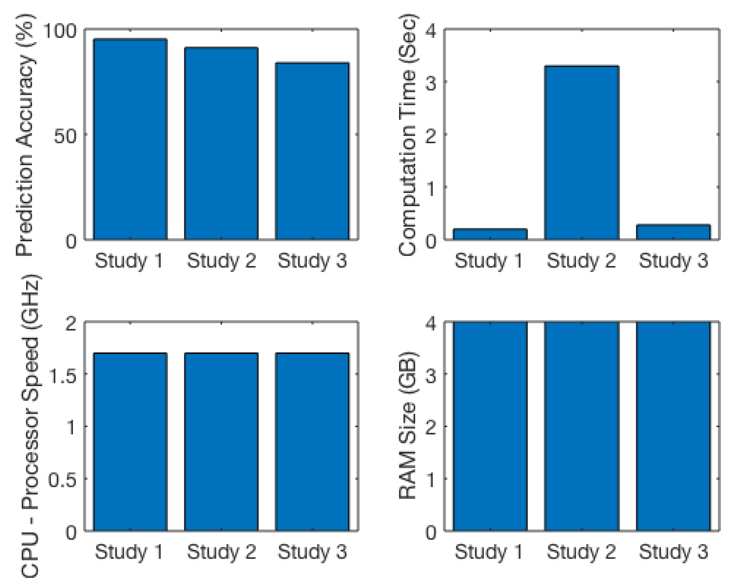
| Study | Experimental Type for Data Collection | Species | Data Size (No of Experimental Observations) | Features/Attributes/Variables | Machine Learning Technique | Algorithms | Prediction Accuracy (Highest) | Computation Time/CPU Time (sec) | Programming Languages, Tools and Computer Details (System Information) |
|---|---|---|---|---|---|---|---|---|---|
| Study 01— Halgamuge (2017) [53] | In vivo (RF-EMF directly expose to whole plants) | Plant | 169 | Species, frequency, SAR, power flux density, electric field strength, exposure durations, and cellular response (presence or absence) | Supervised Machine Learning (classification) | Random Forest, J48, JRip, Random Tree, Bayes Net, Naive Bayes, Decision Table, OneR | 95.26% | 0.2 | MATLAB (MathWorks Inc., Natick, MA, USA) R2015b, one-way ANOVA procedure in SPSS Statistics (Version 23, IBM, Armonk, NY, USA) and Weka tool (Waikato Environment for Knowledge Analysis, Version 3.9, University of Waikato, Hamilton, New Zealand), on computer with 1.7 GHz Intel Core i7 CPU, 4 GB 1600 MHz DDR3 RAM |
| Study 02— Halgamuge and Davis (2019) [54] | In vivo (RF-EMF directly expose to whole plants) | Plant | 169 | Species, frequency, SAR, power flux density, electric field strength, exposure durations, and cellular response (presence or absence) | Supervised Machine Learning (classification) | k-Nearest Neighbor (kNN), Random Forest | 91.17% | 3.38–408.84 | Python 3.6.0 on macOS Sierra (Version 10.12.6), on computer with 1.7 GHz Intel Core i7 CPU, 4 GB 1600 MHz DDR3 RAM |
| Study 03— Halgamuge (2020) (this study) | In-vitro (RF-EMF directly expose to human and animal cells/tissue) | Human and animal cells | 1127 | Species (year of study, human and animal cells/tissue), frequency, SAR, exposure durations, and cellular response (presence or absence) | Supervised Machine Learning (classification) | Random Forest, Bagging, J48, SVM (Linear Kernel), Jrip, Decision Table, BayesNet, Naive Bayes, Logistic Regression | 83.56% | 0.3 | MATLAB (MathWorks Inc., Natick, MA, USA) R2019b and Weka tool (Waikato Environment for Knowledge Analysis, Version 3.9, University of Waikato, Hamilton, New Zealand), on a computer with macOS High Sierra (Version 10.13.6, Apple, Cupertino, CA, USA), on computer with 1.7 GHz Intel Core i7 CPU, 4 GB 1600 MHz DDR3 RAM. |
| Features | Symbol | Type | Feature Type | Description (Domain) |
|---|---|---|---|---|
| Species (human, animal) | c | Nominal | Input | Different cell types have been grouped into two (human or animal cells) |
| Frequency of weak RF-EMF (Hz) | f | Numeric | Input | 800–2450 (MHz) |
| Specific absorption rate, SAR (W/kg) | SAR | Numeric | Input | Up to 50 W/kg—Specific Absorption Rate (SAR) is a proportion of the rate at which energy is absorbed per unit mass by a living organism when exposed to a radiofrequency electromagnetic field (RF-EMF). |
| Duration of exposure time | T | Numeric | Input | 2 min–120 h |
| SAR×exposure time (Halgamuge et al., 2020) [41] | Numeric | Input | Cumulative effect or impact of accumulated SAR within the exposure period | |
| Cellular response (presence or absence) | R | Binary | Output | Presence/Absence |
| No | Affected Cells | Frequency (Hz) | Specific Absorption Rate, SAR (W/kg) | Exposed Time (min) | Radiation Exposure Facility Details |
|---|---|---|---|---|---|
| 1 | Human peripheral blood mononuclear cells (PBMC) | 900, 1800 | 0.024, 0.18, 0.4, 2, 5 | 15, 120, 880 | Waveguide, anechoic chamber, cavity resonator |
| 2 | Human Blood Lymphocytes | 800, 830, 895, 900, 905, 910, 915, 954, 1300, 1800, 1909.8, 1950, 2450 | 0.0054, 0.037, 0.05, 0.18, 0.21, 0.3, 0.5, 0.77, 1, 1.25, 1.5, 2, 2.5, 2.6, 2.9, 3, 3.6, 4.1, 4.3, 5, 6, 8.8, 9, 10, 12.3, 50 | TEM cell, waveguide, horn antenna, wire patch cell (WPC), rectangular waveguide (R18), rectangular waveguide (WR 430), waveguide with cavity resonator, anechoic chamber with horn antenna, trumpet-like aerial | |
| 3 | Human Monocytes, monocytic cells (U937), Human Mono Mac 6 cells (MM6) | 900, 1300, 1800 | 0.18, 0.77, 1, 2, 2.5 | 15, 20, 60, 880 | Rectangular waveguides (R18) with cavity resonator, anechoic chamber with horn antenna |
| 4 | Human B lymphoblastoid cell (TK6, CCRF-CEM) | 1800 | 2 | 40, 480 | Rectangular waveguides |
| 5 | Human T lymphoblastoid cells (Molt-4 T) | 813.5, 836.5, 900 | 0.0024, 0.0026, 0.0035, 0.024, 0.026, 3.2 | 120, 1260, 2880 | TEM cell |
| 6 | Human Leukocytes, human blood neutrophils, human white blood cells | 900, 1800, 1909.8 | 2, 5, 10, 1909.8 | 15, 160, 180, 1440 | TEM cell, waveguide, microstrip transmission line |
| 7 | Human leukemia cells (HL60), human erythroleukemic cells (K562) | 900, 1800, 2450 | 0.000025, 0.000041, 1.8, 2, 2.5, 10 | 120, 180, 240, 360, 480, 880, 1440 | GTEM cell, circular waveguide with cavity resonator, waveguide (TM01) |
| 8 | Human Whole Blood Samples, blood platelets, hemoglobin (HbA), human blood serum | 835, 900, 910, 940, 2375 | 0.24, 0.6, 1, 1.17, 2.4, 12 | 1, 3, 5, 7, 15, 30, 60, 90, 120 | Cavity resonator, spiral antenna setup |
| 9 | Glial cells: Astroglial (astrocytes) cells, astrocytoma cells and microglial cells | 835, 900, 1800 | 1.8, 2.4, 2.5, 12 | 420, 480, 880 | waveguide with cavity resonator |
| 10 | Human glioma cells (LN71, MO54, H4, SHG44) | 900, 954, 2450 | 1.2, 1.5, 5, 10, 50 | 60, 120, 240, 480, 1056, 3000 | GTEM cell, circular waveguide with cavity resonator |
| 11 | Human glioblastoma cells (U87MG, U251MG, A172, T98, U87) | 835 | 2.4, 12 | 420 | |
| 12 | Human neuroblastoma cells (NB69, SK-N-SH, SH-SY5Y, NG108-15) | 872, 900, 1760, 1800, 2200 | 0.023, 0.086, 0.77, 1, 1.5, 1.8, 2.5, 5, 6 | 5, 15, 20, 30, 60, 120, 240, 480, 1440 | Waveguide, wire-patch cell (WPC), waveguide with cavity resonator, chamber with a monopole antenna |
| 13 | Human primary, epidermal keratinocytes, keratinocytes cells (HaCaT) | 900 | 2 | 2880 | Wire-patch antenna |
| 14 | Human fibroblasts, human diploid fibroblasts, human dermal fibroblasts, human skin fibroblasts | 900, 1800, 1950, 2450 | 0.05, 0.2, 1, 1.2, 2, 3 | 20, 60, 80, 320, 480, 580, 2880 | Waveguide, anechoic chamber, wire-patch antenna, rectangular waveguides |
| 15 | Jurkat Cells, Jurkat human T Lymphoma cells | 1800, 2450 | 2, 4 | 160, 2880 | Waveguide, antenna horn |
| 16 | Embryonic carcinoma (EC-P19), Epidermoid carcinoma | 1710, 1950 | 0.0036, 0.4, 1.5, 2 | 60, 120, 180, 480 | Waveguide, waveguide (R14) |
| 17 | Hepatocarcinoma cell line HepG2 | 900, 1800, 2200 | 0.023, 2 | 20, 40, 60, 80, 1440 | Waveguide, horn antena |
| 18 | Human lens epithelial cells (HLECs), eye lens epithelial cells | 1800 | 1, 2, 3, 3.5, 4 | 10, 20, 30, 40, 120, 180, 480, 560, 1440 | Waveguide, rectangular waveguide (R18) |
| 19 | Human epithelial amnion cells (AMA), bronchial epithelial cells (BEAS-2B), human ovarian surface epithelial cells (OSE-80PC), epithelial carcinoma cells, Human HeLa, HeLa S3 | 960, 1800 | 0.0021, 1, 2.1, 3 | 20, 30, 540, 3900 | TEM cell, waveguide, dipole antenna |
| 20 | Human amniotic cell, amniotic epithelial cells (FL) | 960, 1800 | 0.0002, 0.002, 0.02, 0.1, 0.5, 1, 2, 4 | 15, 20, 30, 40, 240 | TEM cell, waveguide |
| 21 | Human breast carcinoma cells (MCF-7) | 900, 1800, 2450 | 0.00018, 0.00036, 0.00058, 0.36, 2 | 60 | Exposure chamber, antenna with falcon tube holder |
| 22 | Human breast epithelial cells (MCF10A), breast fibroblasts | 2100 | 0.607 | 240, 1440 | Horn antenna |
| 23 | Human Spermatozoa | 850, 900, 1800, 1950 | 0.0006, 0.4, 1, 1.3, 1.46, 2, 2.8, 3, 4.3, 5.7, 10.1, 27.5 | 4, 10, 60, 180, 960 | Waveguide, exposure chambers, omni-directional antenna, waveguide in TE10 mode with cavity resonator and monopole antenna |
| 24 | Human Endothelial cells (EA.hy926, EA.hy926v1 and EA.hy296) | 900, 1800 | 0.77, 1.8, 2, 2.2, 2.4, 2.5, 2.8 | 20, 60, 480 | Waveguide, exposure chamber, waveguide with resonator (TE10 mode), waveguide with cavity resonator |
| 25 | Human Trophoblast cells (HTR-8/SV neo cells)/Human lipid membrane (liposomes) | 1800, 1817, 2450 | 0.0028, 0.0056, 2, 38 | 3, 10, 60, 80, 160, 320, 480 | TEM cell, waveguide, dipole antenna, waveguide with cavity resonator |
| 26 | Mast cell lines (HMC-1)—mast cell leukemia | 864.3 | 7 | 140 | Resonant chamber |
| 27 | FC2 cells, human-hamster hybrid cells (AL) | 835, 900 | 0.0107, 0.0172, 2 | 30, 120 | TEM cell |
| 28 | Human adipose derived stem cells | 2450 | 0.24 | 3000 | |
| 29 | Human dendritic cells | 1800 | 4 | 20, 240, 480 | |
| 30 | Human embryonic kidney cells (HEK 293 T) | 940 | 0.09 | 15, 30, 45, 60, 90 | Waveguide |
| 31 | Human umbilical vein endothelial cells (HUVEC) | 1800 | 3 | 20, 500 | Waveguide |
| 32 | Human hair cell, human scalp hair follicle, human dermal papilla cells (hDPC) | 900, 1763 | 0.974, 2, 10 | 15, 30, 60, 180, 420 | Rectangular cavity-type chamber (TE102 mode) |
| No | Affected Cells | Frequency (Hz) | Specific Absorption Rate, SAR (W/kg) | Exposed Time (min) | Radiation Exposure Facility Details |
|---|---|---|---|---|---|
| 1 | Rat primary microglial cells, mouse microglial cells (N9) | 1800, 2450 | 2, 6 | 20, 60, 120, 240 | Waveguide, rectangular horn antenna in an anechoic chamber |
| 2 | Rat glioblastoma cells (C6, C6BU-1) | 1950 | 5.36 | 720, 1440, 2880 | Dipole antenna |
| 3 | Rat astrocytes | 872, 900, 1800, 1950 | 0.3, 0.46, 0.6, 1.5, 2, 2.5, 3, 5.36, 6 | 5, 10, 20, 60, 120, 240, 480, 520, 720, 1440, 2880, 5760 | Waveguide, dipole antenna, horn antenna, rectangular waveguide |
| 4 | Rat brain capillary endothelial cells (BCEC) | 1800 | 0.3, 0.46 | 2880, 5760 | Rectangular waveguide |
| 5 | Mouse neuroblastoma cells (N2a, N18TG-2, NG108-15) | 915 | 0.001, 0.005, 0.01, 0.05, 0.1 | 30 | TEM cell |
| 6 | Rat neurons, murine cholinergic neurons (SN56) | 900, 1800 | 0.25, 1, 2 | 120, 480, 1440, 2880, 4320, 5760, 7200, 8640 | TEM cells, wire-patch cell, rectangular waveguides |
| 7 | Rat/mouse brain cells | 1600, 2450 | 0.00052, 0.23, 0.48, 1.19, 1.2, 2.99, 6.42, 11.21 | Cylindrical waveguide (T11 mode), cylindrical waveguide (T11 mode) | |
| 8 | Rat/mouse bone marrow | 2450 | 12 | 5, 10, 15 | Waveguide |
| 9 | Mouse spermatozoa, Murine spermatocyte-derived cells (GC-2) | 900, 1800 | 0.09, 1, 2, 4 | 20, 5040 | Waveguide, rectangular waveguide |
| 10 | Embryonic mouse fibroblasts cells (C3H10T1/2, NIH3T3, L929), Mouse embryonic skin cells (M5-S), Rat1 cells | 835.62, 847.74, 872, 875, 900, 915, 916, 950, 1800, 2450 | 0.0015, 0.024, 0.03, 0.1, 0.13, 0.24, 0.33, 0.6, 0.91, 1, 2, 2.4, 2.5, 4.4, 5 | 5, 10, 15, 20, 30, 40, 60, 80, 240, 480, 960, 1440, 5760 | Waveguide, radial transmission line, chamber with monopole antenna, magnetron, rectangular waveguide |
| 11 | Mouse embryonic carcinoma cells (P19), Mouse embryonic stem cells, Mouse embryonic neural stem cells (BALB/c) | 800, 1710, 1800 | 1, 1.5, 1.61, 2, 4, 5, 50 | 20, 60, 120 | Waveguide, rectangular waveguide (R18) |
| 12 | Mouse lymphoma cells (L5178Y Tk+/-), Rat basophilic leukemia cells (RBL-2H3), Murine Cytolytic T lymphocytes (CTLL-2) | 835, 915, 930, 2450 | 0.0081, 0.6, 1.5, 25, 40 | 5, 15, 30, 120, 240, 420 | Waveguide, GTEM cell, anechoic chamber, aluminium exposure chamber |
| 13 | Rat granulosa cells (GFSH-R17) | 1800 | 1.2, 2 | 80, 320, 480 | Rectangular waveguides |
| 14 | Rat pheochromocytoma cells (PC12) | 1800 | 2 | 80, 320, 480 | Waveguide |
| 15 | Chinese Hamster Cells (CHO), Ovary (CHO-K1), Chinese hamster lung cells (CHL) | 1800 | 3 | 20, 480 | Waveguide |
| 16 | Chinese hamster fibroblast cells (V79) | 864, 935, 2450 | 0.04, 0.08, 0.12, 0.51 | 15, 60, 120, 180 | TEM cell, GTEM cell |
| 17 | Melanoma cell membrane (B16) | 900 | 3.2 | 120 | Wire patch cell (WPC) |
| 18 | Rat chemoreceptors membranes | 900 | 0.5, 4, 12, 18 | 15 | Waveguide (TE10 mode) |
| 19 | Hamsters pineal glands cells | 1800 | 0.008, 0.08, 0.8, 2.7 | 420 | Radial wave guide |
| 20 | Chick embryos | 915, 2450 | 1.2, 1.75, 2.5, 8.4, 42.6 | 3, 120 | TEM cell, coaxial device |
| 21 | Rabbit lens, Rabbit lens epithelial cells (RLEC) | 2450 | 0.0026, 0.0065, 0.013, 0.026, 0.052 | 480 | TEM cell |
| 22 | Guinea pig cardiac myocytes, pig astrocytes | 900, 1300, 1800 | 0.001 | 8 | TEM cell |
| 23 | Isolated frog auricle | 885, 915 | 8, 10 | 10, 40 | Coplanar stripline slot irradiator |
| 24 | Isolated frog nerve cord | 915 | 20, 30 | ||
| 25 | Snail neurons | 2450 | 0.0125, 0.125, 85 | 30, 45 | Waveguide, waveguide in TE10 mode |
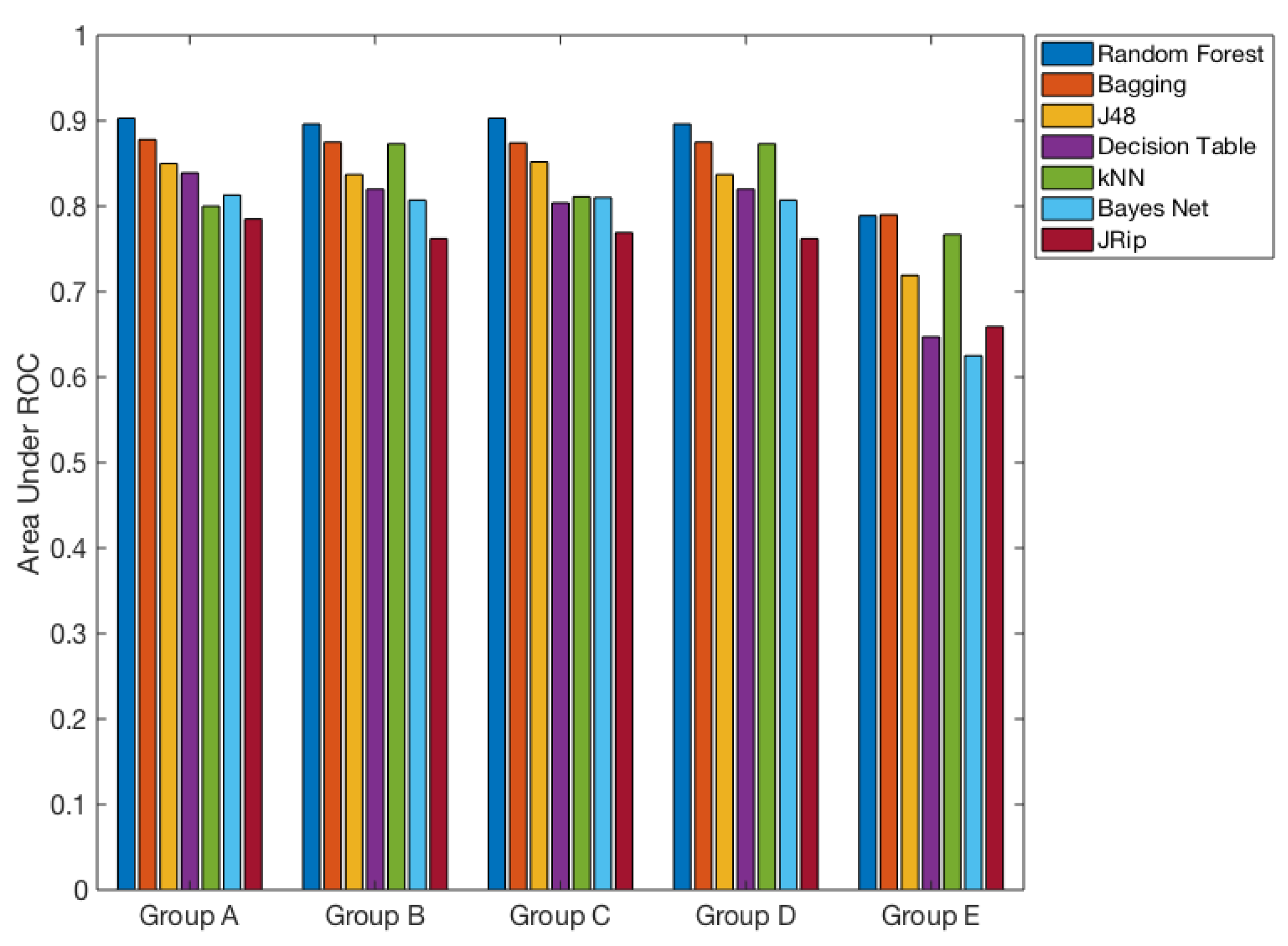
| Group | Selected Features |
|---|---|
| A | Specie, frequency of weak RF-EMF, SAR, exposure time, SAR×exposure time, cellular response (presence or absence) |
| B | Specie, frequency of weak RF-EMF, SAR, exposure time, SAR×exposure time, cellular response (presence or absence) |
| C | Frequency of weak RF-EMF, SAR, exposure time, SAR×exposure time, cellular response (presence or absence) |
| D | Specie, frequency of weak RF-EMF, exposure time, cellular response (presence or absence) |
| E | Specie, SAR, exposure time, SAR×exposure time, cellular response (presence or absence) |
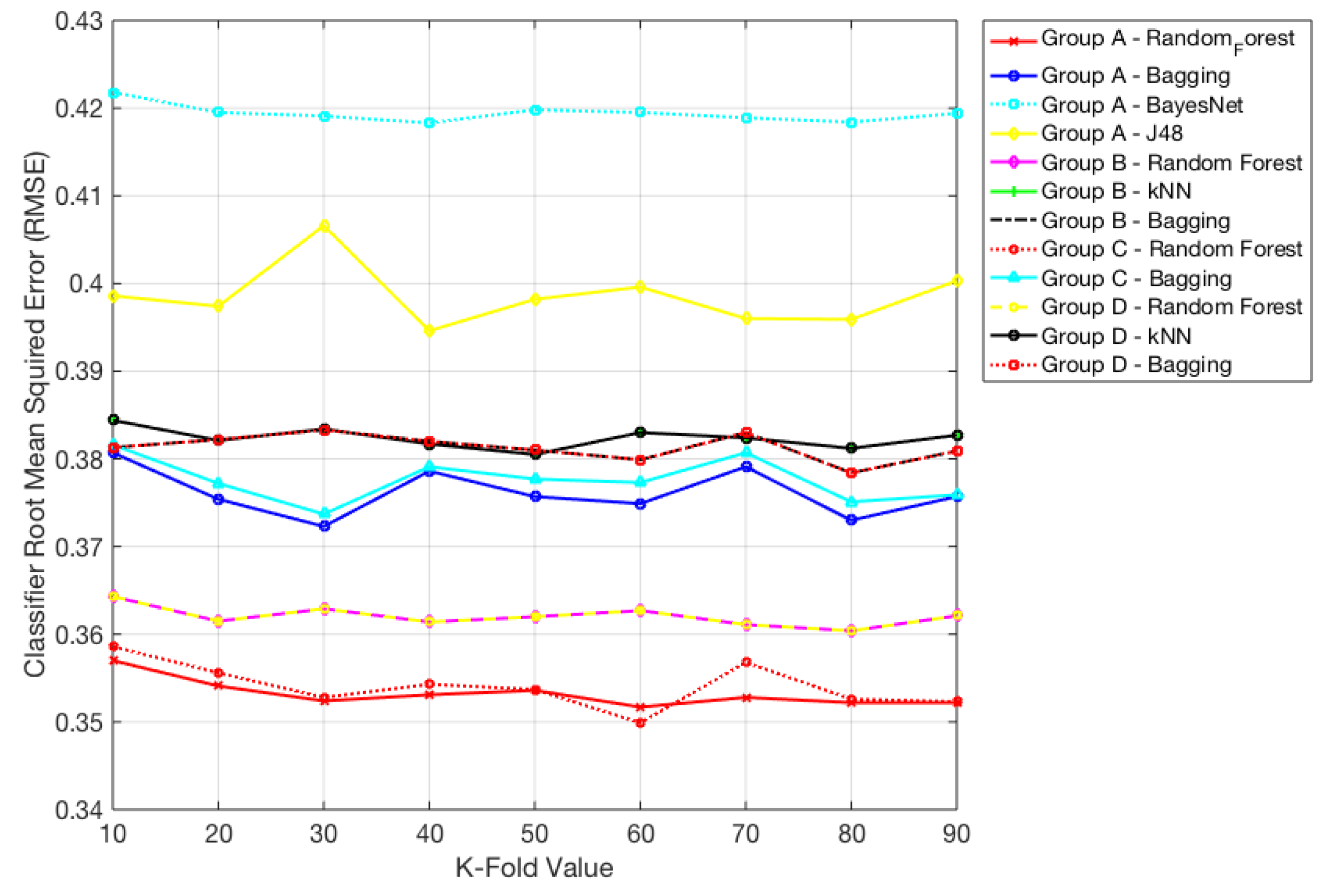
| Group | Model | Fold = 10 | Fold = 20 | Fold = 30 | Fold = 40 | Fold = 50 | Fold = 60 | Fold = 70 | Fold = 80 | Fold = 90 |
|---|---|---|---|---|---|---|---|---|---|---|
| Group A | Random Forest | 82.362 | 82.203 | 83.240 | 83.399 | 82.841 | 83.559 | 83.081 | 83.240 | 83.240 |
| Group A | kNN | 76.457 | 76.696 | 76.856 | 76.696 | 76.856 | 77.015 | 76.935 | 76.536 | 76.616 |
| Group A | Bagging | 79.090 | 79.649 | 80.766 | 79.888 | 79.968 | 80.367 | 79.729 | 80.048 | 81.165 |
| Group A | J48 | 78.532 | 78.851 | 78.133 | 79.649 | 78.931 | 78.611 | 79.729 | 79.249 | 78.691 |
| Group A | Decision Table | 75.579 | 75.658 | 75.419 | 75.020 | 75.738 | 75.579 | 75.977 | 74.940 | 75.179 |
| Group B | Random Forest | 80.447 | 81.484 | 80.607 | 81.006 | 80.766 | 81.165 | 81.804 | 81.405 | 80.926 |
| Group B | kNN | 79.888 | 80.607 | 80.607 | 80.766 | 80.527 | 80.686 | 80.447 | 80.686 | 80.447 |
| Group B | Bagging | 77.574 | 78.292 | 77.494 | 78.452 | 78.532 | 79.329 | 78.053 | 78.931 | 78.372 |
| Group B | J48 | 75.898 | 78.212 | 77.893 | 78.133 | 77.175 | 78.133 | 78.292 | 78.053 | 77.574 |
| Group B | Decision Table | 75.658 | 75.339 | 75.738 | 75.339 | 76.297 | 75.818 | 75.818 | 75.579 | 76.058 |
| Group C | Random Forest | 82.203 | 82.682 | 82.841 | 83.160 | 82.841 | 83.959 | 83.001 | 83.160 | 83.639 |
| Group C | kNN | 78.532 | 78.851 | 78.851 | 79.010 | 79.090 | 79.329 | 79.170 | 78.931 | 78.931 |
| Group C | Bagging | 79.0902 | 79.569 | 79.809 | 79.489 | 79.888 | 80.048 | 79.649 | 79.569 | 79.729 |
| Group C | J48 | 76.377 | 77.175 | 78.053 | 77.095 | 77.095 | 78.452 | 77.334 | 77.813 | 78.212 |
| Group C | Jrip | 75.020 | 75.579 | 75.578 | 75.499 | 74.860 | 75.499 | 74.940 | 75.419 | 76.217 |
| Group D | Random Forest | 80.447 | 81.484 | 80.607 | 81.006 | 80.766 | 81.165 | 81.804 | 81.405 | 80.926 |
| Group D | kNN | 79.888 | 80.607 | 80.607 | 80.766 | 80.527 | 80.686 | 80.447 | 80.686 | 80.447 |
| Group D | Bagging | 77.574 | 78.292 | 77.494 | 78.452 | 78.532 | 79.329 | 78.053 | 78.931 | 78.372 |
| Group D | J48 | 75.898 | 78.212 | 77.893 | 78.133 | 77.175 | 78.133 | 78.292 | 78.053 | 77.574 |
| Group D | Decision Table | 75.658 | 75.339 | 75.738 | 75.339 | 76.297 | 75.818 | 75.818 | 75.579 | 76.056 |
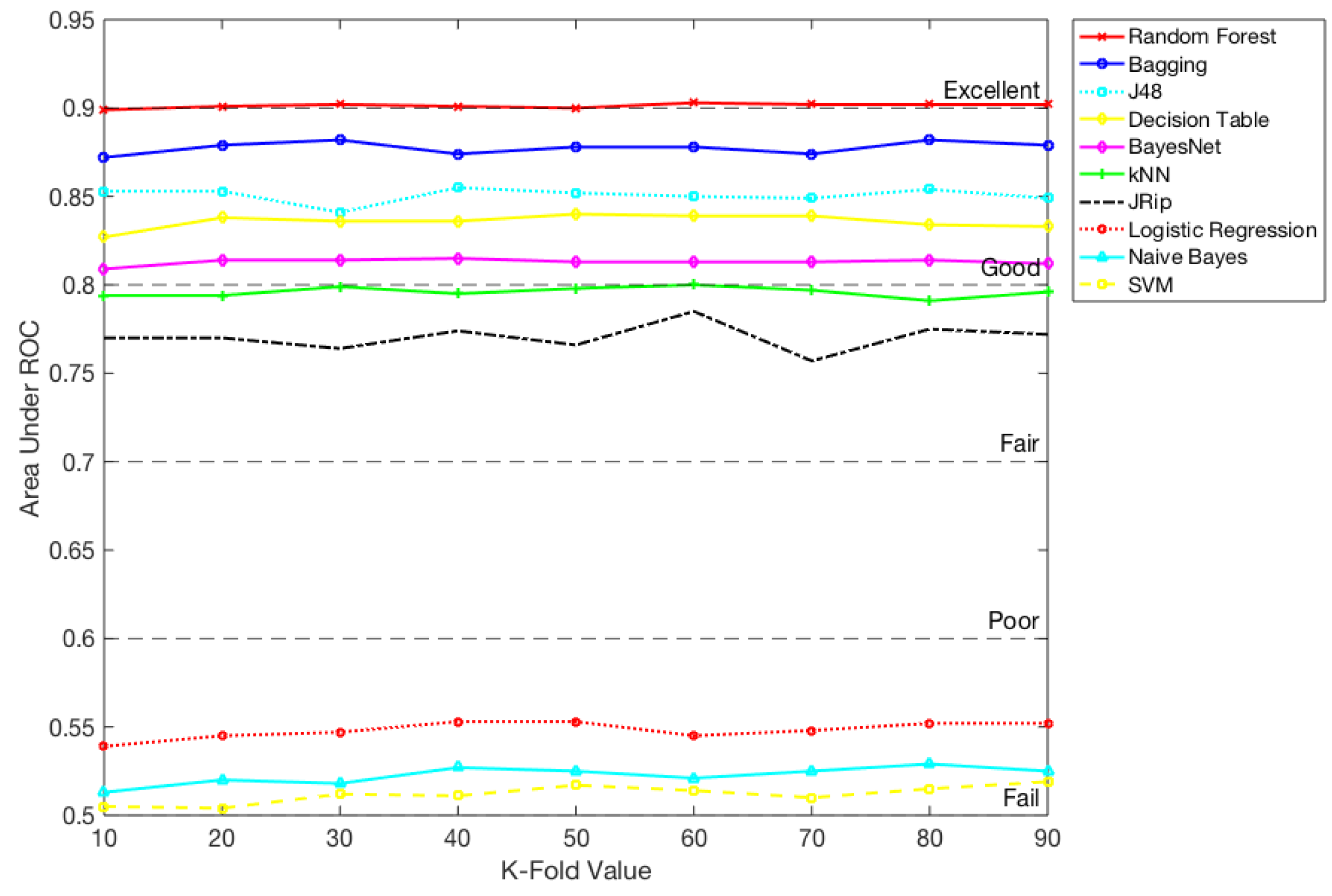
| Group | Model | Fold = 10 | Fold = 20 | Fold = 30 | Fold = 40 | Fold = 50 | Fold = 60 | Fold = 70 | Fold = 80 | Fold = 90 |
|---|---|---|---|---|---|---|---|---|---|---|
| Group A | Random Forest | 0.899 | 0.901 | 0.902 | 0.901 | 0.900 | 0.903 | 0.902 | 0.902 | 0.902 |
| Group A | Bagging | 0.872 | 0.879 | 0.882 | 0.874 | 0.878 | 0.878 | 0.874 | 0.882 | 0.879 |
| Group A | BayesNet | 0.809 | 0.814 | 0.814 | 0.815 | 0.813 | 0.813 | 0.813 | 0.814 | 0.812 |
| Group A | J48 | 0.853 | 0.853 | 0.841 | 0.855 | 0.852 | 0.850 | 0.849 | 0.854 | 0.849 |
| Group A | Decision Table | 0.827 | 0.838 | 0.836 | 0.836 | 0.840 | 0.839 | 0.839 | 0.834 | 0.833 |
| Group B | Random Forest | 0.894 | 0.896 | 0.895 | 0.897 | 0.896 | 0.896 | 0.897 | 0.897 | 0.897 |
| Group B | kNN | 0.873 | 0.874 | 0.873 | 0.876 | 0.877 | 0.873 | 0.874 | 0.875 | 0.873 |
| Group B | Bagging | 0.872 | 0.872 | 0.870 | 0.872 | 0.873 | 0.875 | 0.870 | 0.877 | 0.873 |
| Group B | BayesNet | 0.807 | 0.810 | 0.810 | 0.810 | 0.808 | 0.807 | 0.806 | 0.808 | 0.807 |
| Group B | J48 | 0.834 | 0.841 | 0.838 | 0.841 | 0.838 | 0.837 | 0.832 | 0.837 | 0.834 |
| Group B | Decision Table | 0.822 | 0.819 | 0.818 | 0.815 | 0.815 | 0.820 | 0.813 | 0.812 | 0.822 |
| Group C | Random Forest | 0.895 | 0.898 | 0.902 | 0.899 | 0.900 | 0.903 | 0.897 | 0.902 | 0.901 |
| Group C | kNN | 0.800 | 0.802 | 0.808 | 0.804 | 0.808 | 0.811 | 0.811 | 0.806 | 0.808 |
| Group C | Bagging | 0.870 | 0.876 | 0.881 | 0.874 | 0.876 | 0.874 | 0.872 | 0.88 | 0.878 |
| Group C | BayesNet | 0.808 | 0.813 | 0.812 | 0.812 | 0.810 | 0.810 | 0.810 | 0.809 | 0.809 |
| Group C | J48 | 0.848 | 0.847 | 0.849 | 0.842 | 0.841 | 0.852 | 0.840 | 0.843 | 0.842 |
| Group C | Decision Table | 0.818 | 0.816 | 0.813 | 0.810 | 0.812 | 0.804 | 0.811 | 0.811 | 0.813 |
| Group D | Random Forest | 0.894 | 0.896 | 0.895 | 0.897 | 0.896 | 0.896 | 0.897 | 0.897 | 0.897 |
| Group D | kNN | 0.873 | 0.874 | 0.873 | 0.876 | 0.877 | 0.873 | 0.874 | 0.875 | 0.873 |
| Group D | Bagging | 0.872 | 0.872 | 0.870 | 0.872 | 0.873 | 0.875 | 0.870 | 0.877 | 0.873 |
| Group D | BayesNet | 0.807 | 0.810 | 0.810 | 0.810 | 0.808 | 0.807 | 0.806 | 0.808 | 0.807 |
| Group D | J48 | 0.834 | 0.841 | 0.838 | 0.841 | 0.838 | 0.837 | 0.832 | 0.837 | 0.834 |
| Group D | Decision Table | 0.822 | 0.819 | 0.818 | 0.815 | 0.815 | 0.820 | 0.813 | 0.812 | 0.822 |
| Classification Modle | PCC | RMSE | Precision | Sensitivity or Recall | (1− Specificity) | Area under the ROC Curve | Precision-Recall (PRC Area) |
|---|---|---|---|---|---|---|---|
| Random Forest | 83.559 | 0.352 | 0.815 | 0.843 | 0.829 | 0.903 | 0.878 |
| kNN | 77.015 | 0.456 | 0.748 | 0.774 | 0.767 | 0.800 | 0.741 |
| Bagging | 80.367 | 0.375 | 0.783 | 0.809 | 0.799 | 0.878 | 0.845 |
| SVM | 52.514 | 0.689 | 0.496 | 0.319 | 0.709 | 0.514 | 0.480 |
| Naive Bayes | 51.317 | 0.563 | 0.313 | 0.025 | 0.950 | 0.521 | 0.472 |
| Bayes Net | 74.701 | 0.419 | 0.746 | 0.704 | 0.785 | 0.813 | 0.782 |
| J48 | 78.611 | 0.399 | 0.752 | 0.816 | 0.759 | 0.850 | 0.803 |
| Jrip | 75.020 | 0.428 | 0.745 | 0.716 | 0.781 | 0.785 | 0.772 |
| Decision Table | 75.579 | 0.403 | 0.731 | 0.764 | 0.749 | 0.839 | 0.792 |
| Logistic Regression | 52.993 | 0.498 | 0.505 | 0.275 | 0.758 | 0.545 | 0.486 |
© 2020 by the author. Licensee MDPI, Basel, Switzerland. This article is an open access article distributed under the terms and conditions of the Creative Commons Attribution (CC BY) license (http://creativecommons.org/licenses/by/4.0/).
Share and Cite
Halgamuge, M.N. Supervised Machine Learning Algorithms for Bioelectromagnetics: Prediction Models and Feature Selection Techniques Using Data from Weak Radiofrequency Radiation Effect on Human and Animals Cells. Int. J. Environ. Res. Public Health 2020, 17, 4595. https://0-doi-org.brum.beds.ac.uk/10.3390/ijerph17124595
Halgamuge MN. Supervised Machine Learning Algorithms for Bioelectromagnetics: Prediction Models and Feature Selection Techniques Using Data from Weak Radiofrequency Radiation Effect on Human and Animals Cells. International Journal of Environmental Research and Public Health. 2020; 17(12):4595. https://0-doi-org.brum.beds.ac.uk/10.3390/ijerph17124595
Chicago/Turabian StyleHalgamuge, Malka N. 2020. "Supervised Machine Learning Algorithms for Bioelectromagnetics: Prediction Models and Feature Selection Techniques Using Data from Weak Radiofrequency Radiation Effect on Human and Animals Cells" International Journal of Environmental Research and Public Health 17, no. 12: 4595. https://0-doi-org.brum.beds.ac.uk/10.3390/ijerph17124595